Jun 3, 1993 - methods (Mason et al., 1975; Panda and. Rosenfeld, 1978) take into ..... Satellite Cloud Photography. Proc. Third Symp. on ..... SECURITY.
NASA Technical
Memorandum
104022
A Summary of Image Segmentation Techniques Lilly Spirkovska,
Ames Research
June 1993
National Aeronautics and Space Administration Ames Research Center Moffett Field, California 94035-1000
Center, Moffett
Field, California
Summary Machine vision systems are often considered to be composed of two subsystems: low-level vision and highlevel vision. Low-level vision consists primarily of image processing operations performed on the input image to produce another image with more favorable characteristics. These operations may yield images with reduced noise or cause certain features of the image to be emphasized (such as edges). High-level vision includes object recognition and, at the highest level, scene interpretation. The bridge between these two subsystems is the segmentation system. Through segmentation, the enhanced input image is mapped into a description involving regions with common features which can be used by the higher level vision tasks. There is no theory on image segmentation. Instead, image segmentation techniques are basically ad hoc and differ mostly in the way they emphasize one or more of the desired properties of an ideal segmenter and in the way they balance and compromise one desired property against another. These techniques can be categorized in a number of different groups including local vs. global, parallel vs. sequential, contextual vs. non contextual, interactive vs. automatic. In this paper, we categorize the schemes into three main groups: pixel-based, edge-based, and regionbased. Pixel-based segmentation schemes classify pixels based solely on their gray levels. Edge-based schemes first detect local discontinuities (edges) and then use that information to separate the image into regions. Finally, region-based schemes start with a seed pixel (or group of pixels) and then grow or split the seed until the original image is composed of only homogeneous regions. Because there are a number of survey papers available, we will not discuss all segmentation schemes. Rather than a survey, we take the approach of a detailed overview. We focus only on the more common approaches in order to give the reader a flavor for the variety of techniques available yet present enough details to facilitate implementation and experimentation.
Introduction Machine vision systems are often considered to be composed of two sub-systems: low-level vision and highlevel vision. Low-level vision consists primarily of image processing operations performed on the input image to produce another image with more favorable characteristics. These operations may yield images with reduced noise or cause certain features of the image to be emphasized (such as edges). High-level vision includes object
recognition and, at the highest level, scene interpretation. The bridge between these two subsystems is the segmentation system. Through segmentation, the enhanced input image is mapped into a description involving regions with common features which can be used by the higher level vision tasks. On one hand, this procedure should be sensitive enough to extract those areas of interest in the image. On the other hand, it should be immune to the disturbances of irrelevant objects and noise in the system. Ideally, a good segmenter should produce regions which are uniform and homogeneous with respect to some characteristic such as gray tone or texture yet simple, without many small holes. Further, the boundaries of each segment should be spatially accurate yet smooth, not ragged. And finally, adjacent regions should have significantly different values with respect to the characteristics on which region uniformity is based. This situation can be represented mathematically as follows: If I is the set of all pixels and PO is a uniformity predicate defined on groups of connected pixels, a segmentation of I is a partitioning set of connected subsets or image regions {R 1, R 2 ..... Rn} such that n
URl=I, 1=1
whereRl_'qRm=O
and the uniformity level) satisfies
predicate
Vl_m
(such as nearly
equal gray
P(RI) = True V1 P( R1U
Rm) = False,
(2)
_/R 1 adjacent to Rm
(R1D Rm) ^ (Rm * O) ^ (P(RI)
(1)
(3)
= True) ::_ P(Rm)
(4) = True Because noise destroys homogeneity in a local context, it is not possible to determine a consistent homogeneity of larger regions, resulting in fragmented segmentation results. If noise characteristics are known, however, it is possible to determine homogeneity on statistical grounds. In this case, we must drop the consistency criterion given by equation (4) which states that if a region is homogeneous, then all subsets of this region will also be homogeneous. This means that a region may be determined to be homogeneous even when subsets of this region are not. There is no theory on image segmentation. Instead, image segmentation techniques are basically ad hoc and differ mostly in the way they emphasize one or more of the desired properties of an ideal segmenter and in the way they balance and compromise one desired property
against another. These techniques
can be categorized in a number of different groups including local vs. global, parallel vs. sequential, contextual vs. non contextual, interactive vs. automatic. In this paper, we categorize the schemes into three main groups: pixel-based, edge-based, and region-based. Pixei-based segmentation schemes classify pixels based solely on their gray levels. Edgebased schemes first detect local discontinuities (edges) and then use that information to separate the image into regions. Finally, region-based schemes start with a seed pixel (or group of pixels) and then grow or split the seed until the original image is composed of only homogeneous regions. Because there are a number of survey papers available (Sahoo et al., 1988; Weszka, 1978; Haralick and Shapiro, 1985), we will not discuss all segmentation schemes. Rather than a survey, we take the approach of a detailed overview. We focus only on the more common approaches in order to give the reader a flavor for the variety of techniques available yet present enough details to facilitate implementation and experimentation.
Pixel-Based
Segmentation
Schemes
Gaussian _tering algorithmThe simplest segmentation method is based on the Bayes decision theory in pattern recognition. The gray level histogram of the image is computed and then two component densities are extracted (corresponding to the object and the background) from the mixture density associated with the histogram. It is commonly assumed that both the background and the object densities are Gaussian. Algorithm: 1. Compute the mean ([.t) and standard deviation the histogram: I _
(c) of
(5)
F(i)* i
c = _l_F(i)*
(i-l.t)
2
(6)
where F(i) is the histogram value for gray level i (out of L gray levels) and N is the number of points in the window. To avoid the problem of division by 0 (for the deviation is necessarily 0 for 1-pixel regions and regions having identically valued pixels), a small positive constant can be added to a. 2.
Find a least-squares
fit of
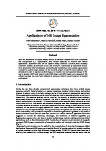
Mode Method The most widely used segmentation technique is the mode method which is applicable to images with bimodal histograms, as shown in figure 1. One mode of the histogram corresponds to the gray levels of the object pixels while the other mode captures the gray levels of the background pixels. It is assumed that a fixed threshold level exists that separates the background area from the objects. The threshold level is chosen to be the gray level in between the two modes using any of a number of different methods. The two most popular methods are Gaussian filtering (Jain and Dubuisson, 1992) and Otsu's method based on discriminant
analysis
(Otsu,
1979).
P! ---(i-I'tl)2/2_2 f(i) = _11 {_
+ P2
to the histogram F(i) by adjusting _1, P2, _2, _2 as follows: (i) Smooth average:
the histogram
(8) On the smoothed histogram, find the deepest valley v (= lowest value) and use it to divide the histogram into two parts. Compute initial estimates of P1, I-tl, _1, P2, I-t2, and a2 on these two parts (for the original histogram F(i)): L N2=
i=l
1: A bimodal histogram. One mode represents the background pixels while the other represents the object pixels.
(9)
_F(i) i=v+l
v
Gray levels Figure
P1, _tl,
F'(i) = F(i - 2) +2F(i - 1) + 3F(i) + 2F(i + 1) + F(i + 2) 9
N 1 =EF(i),
_t.
the parameters
(7)
by taking a local weighted
v o_
-(i-la*)2/2c2 -
_tI =
L F(i) * i,
"=
Is2 = -F(i)* N2 i=v+l
i
(10)
el=
F(i)* (i- It1)2
(11)
F(i)* (i - It2)2 i=v+l
(12)
_
c2 =
Otsu's algorithmOtsu's method of determining a threshold in a bimodal histogram is based on discriminant analysis in which thresholding is regarded as the partitioning of the pixels of an image into two classes C O and C 1 at gray level t. Algorithm: n i = number
of pixels at level i (from L gray levels)
N = total number
g2 =
F(i)* (i -g2) 2 i=v+l
_
(13)
of pixels = n I + n2 + ..- + nL
1. The gray level histogram as a probability distribution:
(ii) Useahill-climbing method tominimize: L Z
[f(i) - F(i)] 2
i=l
(b)
Calculate:
left_val
(c)
Calculate:
right_val
(d)
If (left_val
_0
(19)
Pi =1
(20)
i=l
valley
Dichotomize pixels into two classes CO and C1 by a threshold at level k. ,
1)1.
3.
+ 1)1.
Calculate
the probabilities
of class occurrence: k
for deepest w 0 = Pr (Co) = Z
1.
Else if (right_val deepest
= If(i-
< val), set the estimate
(21)
w(k)
Pi
i=l
for
L
valley at i + 1. Else deepest
and regarded
L
(14)
(a) Calculate: val = If(i) - F(i)l for i = deepest (v) chosen in step (i) or (ii.d).
is normalized
valley found
w 1 = Pr (C1) =
at i.
ZPi
= 1 - w(k)
(22)
i=k+l (e) If the deepest valley value was changed in step (d), reestimate P1, Itl, _1, P2, It2, and a2 using equations (9-13) and the new value of v. Repeat steps (a-d).
4.
Calculate
the class mean levels:
k
k It(k)/w(k)
It0 = __._ i Pr(i IC 0) = Zipi/w0 3. After the parameters of the mixture density have been estimated, a pixel with gray level x is assigned to the object if
(15)
i=l
(23)
i=l L
L
Itl = ZiPr(ilCi)= i=k+l
ZiPi/Wi i=k+l
(24)
= (itT- It(k)) I(I- w(k)) The threshold
value t is then defined
PI _-(t-gl)2/2°l _111 _
2
P2=_22e
as -(t-g2)2/2°22 (16)
where w(k) and It(k) arethezeroethand first-order cumulativemorncntsof thehistogramup tothekth level and L
and satisfies: _tl=
12/22
Itl ('_2
123t2+2(it2_O2
. , Itl
It2 +,_1_ P2(_I = 0
ZiPr(ilCl)= i=k+l = (itT - It(k))/(1
L ZiPi/Wl i=k+l - w(k))
(17) is the total mean level of the original
picture.
(25)
5.
Calculate
class variances:
Thus, the optimal threshold maximizes o2(k).
k (i -_t0)
2 Pr(i IC0) = __..,(i-
i=l
2 Pr(i ICI)=
_(i-btl)
i=k+l
2 pi/wl
(27)
i=k+l
6. In order to evaluate the "goodness" k, we can use the following discriminant (or measures
of the threshold criterion
of class separability):
-2, --
o2 _ = o v' o2
(28)
where 02 is the within-class
= wo o2 + Wl o2
(29)
variance,
0 2 = w0(l.t 0 -I.tT) 2 +Wl(g
1 -gT)
2
(30) = W0Wl (it I _ _t0)2 is the between-class
variance,
and
L 02
= _ (ii=l
gT) 2 Pi
(31)
is the total variance. Note that X, r,, and r I are equivalent given k because 02
+ 02
to one another
= 02
(32)
to an optimization k that maximizes one of
the,,object
measures).
OT2is independent of k. Further, 0 2 is based on secondorder statistics while 02 is based on first-order statistics. measure
with
Since o 2 is independent maximizing o2(k): o2(k)
4
discussed
above
a2
of k, we can maximize
= [btTw(k)I't(k)]2 w(k)[l - w(k)]
distribution (intensity level, and the noise is fail when it is difficult images with extremely broad and flat valleys.
noise) is independent of the gray spatially uncorrelated. The methods to detect the valley bottom, as in unequal peaks or in those with Since peaks tend to become wider
and lower with an increasing amount of intensity noise, some sharpening of the peaks and valleys can be accomplished by applying noise reduction preprocessing procedures. Another approach to sharpening peaks and valleys is to weigh the influence of individual pixels and not count them all equally when calculating the histogram, as in the gradient-guided methods. Gradient guided histograms take one of two forms, interior only or boundary only. The interior-only methods (Mason et al., 1975; Panda and Rosenfeld, 1978) take into account only pixeis belonging to either the objects or the background (i.e., those pixels having low gradient values), disregarding pixels belonging to boundaries where the gray level varies rapidly. This should yield a histogram with sharper peaks and deeper valleys. In contrast, the boundary-only methods (Weszka, Nagel, and Rosenfeld, 1974; Watanabe et al., 1974) take into account only pixels belonging to boundaries (i.e., those pixels having high gradient values). This should yield a well-defined unimodal histogram, the peak value of which is a proper constant threshold level. Finally, instead of computing a 1D histogram of gray level values, a 2D histogram or "scatter" diagram can be computed with gray level and gradient as its coordinates. In this case, a good threshold can be selected using clusters of points rather than the modes of a histogram (Katz, 1965; Weszka and Rosenfeld, 1979). Local methodsGlobal segmentation techniques such as the mode method are notoriously sensitive to parameters like ambient illumination, object shape and size, noise level, variance of gray levels within the object and background, and contrast (Taxt et al., 1989). When there is a large range of variation in gray values from one part of the image to the other, a single threshold value cannot
_ o__ .2B _-
methods
Note that
o_v and of 3 are functions of threshold level k, whereas
Thus, we use TIsince it is the simplest respect to k:
determination
for a
7. The problem is now reduced problem to search for a threshold functions,, (the criterion
The threshold
work well when the object size is large enough to make a distinct mode in the histogram, the gray level noise
L
_(i-gl)
measures
(26)
i=l
L
4--
_t0) 2 Pi/W0
t is chosen to be that k which
(33) 1"/by
(34)
be used. Further, objects may legitimately have widely different albedos and, as a result, an object in one part of an image may be lighter than the background in another part. Local methods attempt to eliminate these disadvantages by partitioning the image into mining a threshold for each of these then smoothing between subimages tinuities. An example of this group
subimages, detersubimages, and to eliminate disconof methods is the
Chow-Kaneko adaptive thresholding method (Chowand Kaneko, 1972). Thismethod assigns adifferent threshold valuetoeachpixei. Chow-Kaneko adaptive thresholding algoritlun-
or entirely on background areas, by chance yield subhistograms that are judged to be bimodal.
1.
Edge-based information
Subdivide
the image into several
subimages.
2. For each subimage, compute the histogram, smooth it, and determine a threshold using the mode method. 3.
Smooth
the thresholds
among
Determine
For example,
a threshold to interpolate
the neighboring
for each pixel by interpolation. the 2 x 2 image:
[:,701 into a 4 x 4 image, begin in the columns form a 2 x 4 image:
[_
567] 89
segmentation into account
Schemes
schemes also take local but do it relative to the contents
regions. The most direct method is the detect and link method in which local discontinuities are first detected and then connected to form longer, hopefully complete, boundaries. The disadvantage of this approach is that the edges are not guaranteed to form closed boundaries and thus the subsequent thresholding scheme merges regions which may not be uniform (relative to the uniformity
direction
and
predicate
discussed
in the introduction).
An improvement over this method is Yanowitz and Bruckstein's adaptive thresholding method (Yanowitz and Bruckstein, 1989). Similar to the detect and link
10
in the rows direction,
Then interpolating
Segmentation
of the image, not based on an arbitrary grid. Each of the methods in this category involves finding the edges in an image and then using that information to separate the
subimages. 4.
Edge-Based
form the desired
4 x 4 image:
method, the adaptive thresholding method locates objects in an image by using the intensity gradient. These edges are used as a guide to determine an initial threshold level for various areas of the image. Local image properties are then used to assign thresholds to the remainder of the image.
[_
5.
Threshold
assigned
56i]67891087
the image using the threshold
Another improvement of the detect and link method is the local intensity gradient (LIG) method (Parker, 1991). It is similar to Yanowitz and Bruckstein's algorithm and
value
works
to each pixel.
The biggest determinant of whether a local thresholding method produces an acceptable segmentation is the size of the subwindows. If it is chosen to be too large, the algorithm will not focus on local properties and will not perform significantly better than global techniques. On the other hand, if it is chosen to be too small, the histograms produced for each subwindow would yield meaningless statistics since the number of pixels participating in the process would be reduced substantially. Unfortunately, the best method of choosing an appropriate window size is by trial-and-error. Even if window
size is chosen well, the grid imposed
well in practice.
Yanowitz
would
be set at arbitrary
locations
instead
grid windows
placed
entirely
on object areas
Thresholding
2. Derive the gray-level gradient magnitude image from the smoothed original. In discrete images, the gradient is actually computed distance:
as an intensity
difference
over a small
G(i, j) = min(I(i, j) - I(i + _i, J + _Sj))
(35) _i =-1,1,
of
Adaptive
below.
1. Smooth the image, replacing every pixei by the average gray-level values of some small neighborhood of it.
on
being placed in truly meaningful positions. Purely local techniques are blind to trends in the data that are significantly larger than their element size. Finally, serious errors can occur if, due to noise and bad lighting conditions,
and Bruckstein's
each algorithm
Algorithm
the image may not be coherent with the image contents and thus the threshold values determined within a subwindow
We present
_ij =-1,I
where I is the image being examined and G is the resulting image consisting of differences. 3. Thin the gradient image, keeping only points in the image which have local gradient maxima. This should produce
a one-pixel
wide edge.
4. Sample thesmoothed imageatthese maximal gradient (oredge) points.These pointsareassumed tobe correct. 5. Interpolate thesampled graylevelsovertheimage. Theresultis athreshold surface, witha(possibly) differentthreshold valueforeachpixel. 6. Usingtheobtained threshold surface, segment the image. If theoriginalpixelvalueisgreater thanorequal tothethreshold valueatthatlocation, setthethresholded valueto 1(orwhite).Otherwise, setthevalueto0 (or black).Thus,objects will besettowhiteandbackground toblack. Local Intensity
Gradient
The local intensity
Method
gradient
method
Algorithm (Parker, 1991) is
based on the fact that objects in an image will produce small regions with a relatively large intensity gradient (at the boundaries of objects) whereas other areas ought to have a relatively small gradient. It uses small subimages of the gradient image to find local means and deviations. As in the local mode techniques, these regions must be small enough so that the illumination effects can be ignored. 1.
Compute
a smooth
gradient
of the image.
• For all pixels in the N x N image (IM1), compute the minimum difference between the pixel and all eight neighbors. (See gradient computation in step 2 of Yanowitz and Bruckstein's algorithm.) Store in IM2. • Break up IM2 (gradient array) into subregions, each composed of M x M pixels. Compute the mean value (QIM) and mean deviation (QDEV) for each subregion k:
QIM[k]
QDEV[k]--
1 = M*M
M _
i=l
j=l
IM2[i] [j]
•
(IM2[i][j]-QIM[k])
(38)
2 (39)
i--I j=l • Smooth both QIM and QDE¥. The value of QIM (and QDEV) at each point is replaced by the weighted mean of all the neighboring subregions using the following weight matrix:
1.0 0.7 0.7
1.5 1.0 1.0
1.0 0.7] 0.7
2. Find the object pixels in the gradient image. Object pixels are defined as outliers in the smoothed image. That is, pixel [i,j] is an object pixel if IM2[ij] < QIM[i,j] + 3*QDEV[ij]. Otherwise [i,j] is unclassified. 3. After sample object pixels are found, thresholds can be identified for the remaining pixels. This can be done using a region growing procedure based on gray levels in the local surroundings, and begins at pixels that are known to belong to the object. • For all unclassified pixels [i,j], select a gray level threshold by finding the smallest gray level value in an 8-neighborhood (pixel aggregation). If IM 1[i j] is less than this value, it is an object pixel. Repeat until no more object pixels are found. • (Optional) For all still unclassified pixels, compute a threshold as the mean of at least four neighboring object pixels (region growing). Repeat until no new object pixels are found. • (Optional) For all still unclassified pixels, compute a threshold as the minimum of at least six neighbors (region growing). Repeat until no new object pixels are found. 4. Set all object pixels in IM1 to the value 0 and all unclassified pixels to a positive value. IM1 now contains the thresholded image.
Region-Based
M
_
• Interpolate/extrapolate the values of QIM and QDEV to fill an N x N region again. Linear interpolation is acceptable. This results in an image containing estimates of the gradient and deviation at each pixel.
Segmentation
Schemes
Region-based segmentation schemes attempt to group pixels with similar characteristics (such as approximate gray level equality) into regions. Conventionally, these are global hypothesis testing techniques. The process can start at the pixel level or at an intermediate level. Generation confidence
and filtering of good seed regions of high is essential. Given initially poor or incorrect
seed regions, these techniques usually do not provide any mechanism for detecting and rejecting local gross errors in situations such as when an initial seed region spans two separate surfaces. These techniques can also fail if the definition of region uniformity is too strict, such as when we insist on approximately constant brightness while in reality brightness may vary linearly. Another potential problem with region growing schemes is their inherent dependence on the order in which pixels and regions are examined. Usually, however, differences caused by scan order are minor.
Therearetwoapproaches inregion-based methods: regiongrowingandregionsplitting. Intheregion growingmethods, theevaluated setsareverysmallatthe startofthesegmentation process. Theiterative process of regiongrowing mustthenbeapplied inordertorecover thesurfaces ofinterest. Intheregiongrowing process, the seed regionisexpanded toinclude allhomogeneous neighbors andtheprocess isrepeated. Theprocess ends whentherearenomorepixelstobeclassified. Because initialseeds areverysmall,theprocessing timecanbe minimized byminimizing thenumber oftimesanimage element isusedtodetermine thehomogeneity ofaregion. Inregionsplittingmethods, ontheotherhand,the evaluation ofhomogeneity ismade onthebasisoflarge setsofimageelements. Theprocess starts withtheentire imageastheseed. If theseedisinhomogeneous, it is split intoapredetermined number ofsubregions, typically four.Theregionsplittingprocess isthenrepeated using eachsubregion asaseed. Theprocess endswhenall subregions arehomogeneous. Because theseeds being processed ateachstepcontain manypixels,region splittingmethods arelesssensitive tonoisethanthe regiongrowing methods. Inbothapproaches, their iterative structure leadstocomputationally intensive algorithms. Inthelate70s,Horowitz andPavlidis developed ahybrid algorithm, thesplit,merge, andgroup(SMG)algorithm (Horowitz andPavlidis,1976; ChenandLin,1991), whichincorporates theadvantages ofbothapproaches. Because theSMGalgorithm begins atanintermediate resolution level,it ismoreefficientthaneitherthepure splitalgorithms orthepuremerge algorithms. Themajor disadvantage, however, isthattheresulting imagetends tomimicthedatastructure usedtorepresent theimage (aquadtree for2Dimages oranoctree orK-treefor 3Dimages) andcomes outtoosquare. Split,Merge, 1.
and Group
Initialization
in terms of minimizing
the expected
number
of
splits and merges. 2.
Merge
phase:
If level Ls is homogeneous,
evaluate
the homoge-
neity of level Ls + 1. If the node is homogeneous, the four children are cut and the node becomes an endnode. Repeat until no merges take place or level n is reached (a homogeneous image). 3.
Split phase:
If level Ls is inhomogeneous, split the nodes into four children and add them to the quadtree. Evaluate the new endnodes and if necessary, split again until the quadtree 4.
has homogeneous
Conversion
endnodes
from quadtree
only.
to RAG phase:
* A RAG is a Region Adjacency Graph. It allows different subimages that are adjacent but cannot be merged in the quadtree to be merged. • This phase consists of extracting the implicit adjacency relations from quadtree endnodes needed to construct the branches of the RAG. Two neighboring subimages in the quadtree will have common ancestors, i.e., nodes in the quadtree on a higher level from which both endnodes can be reached.
Next, the path is mirrored about an axis formed by the common boundary between the adjacent subimages.
Divide the image into subimages using a quadtree structure, as shown in figure 2. The root of the quadtree corresponds to the whole image. Each node in the quadtree has only one parent (except for the root) and four children (except for the leaves). The four children are denoted by the quadrant within the parent that they correspond to (NW, NE, SW, SE). Thus, the image must be 2 n × 2 n pixels. The leaves are at node level 0. The root is at level n. During initialization, the quadtree is built from the root down to a heuristically set initialization of the initialization
selected
• First, the nearest common ancestor is determined that connects the current endnode with the neighbor.
Algorithm
phase:
level Ls. The choice
Figure 2: (a) Original image split using quadtree. (b) Quadtree representation of image.
level L s can be
5.
Grouping
phase:
The now explicit neighbor relationships can be used to merge adjacent nodes which have a homogeneous union. Grouping strategies include: a. Assign the first node of the RAG (corresponding with the subimage in the top left corner) the status of seed. The neighbors of the seed are then evaluated on homogeneity together with the seed. A merge of a neighbor with the seed produces new neighbors, which are evaluated. When no more grouping takes place, the
seedisrendered inactive andanewseed(thefirst unprocessed node)isassigned. Thegrouping phase ends if allremaining RAGnodes havebecome inactive. b. Sequential grouping: theseeds arechosen based ontheirsizewiththefirstseed beingthelargest subimage, etc.A disadvantage ofthisapproach isthat because ofthesizeofthefirstseed, these regions tendto growbeyond their"actual"boundaries, annexing all fuzzyborderareas. c. Parallel grouping: assign anumber ofactive seeds atthestartofthegrouping phase. Nowonlydirect neighbors ofaseed aregrouped if possible. New neighbors havetowaltforevaluation untiltheseedis processed again.Activeseeds areprocessed successively untilnoneremain. Thegrowing ofseeds will bebounded byotherseeds. Grouping strategy (a)issufficient inpractice. 6. Postprocessing oftheRAGphase: • If subimages aretoosmall,merge themwith their nearest neighbor. It is regions as objects and large number of them, computational burden
difficult to interpret very small since there is usually a relatively their presence increases the on later stages of processing.
• Exploit prior knowledge about the application problem to improve the segmentation.
Concluding
Remarks
The goal of image segmentation is a domain-independent decomposition of an image into distinct regions which are uniform in some measurable property such as brightness, color, or texture. Unfortunately, natural scenes often contain feature gradients, highlights, shadows, textures, and small objects with fine geometric structure, all of which make the process of producing useful segmentations extremely difficult. We have presented some of the techniques which attempt to deal with these difficulties. Although they produce reasonable segmentations in many situations, at some point local ambiguities and errors introduced by the segmentation process can only be resolved by application specific knowledge. Since the quality of the above segmentation techniques depends on the type of image the technique is being applied to, we will end this overview with a summary of what type of image each technique works best on. • The mode method is applicable to images with bimodal histograms where the modes are fairly distinct (well separated
and sharp)
and of nearly equal length.
It does
not work well if the gray level noise distribution is dependent on the gray level or is spatially correlated. • Local methods, such as the Chow-Kaneko method, are applicable to images in which the ambient illumination may vary in gray level from one part of the image to another or when one part of an image may be lighter than the background in another (as long as the contrast in each area is adequate). The major disadvantage of local methods is that it is difficult to choose an appropriate window size which localizes the illumination variation yet considers a large enough area to yield meaningful statistics. Also, even if the window size is chosen well, the grid imposed on the image may not be coherent with the image contents and thus threshold values determined within a subwindow would be set at arbitrary positions instead of being placed in truly meaningful positions. • Because the quality of the segmentation depends on the quality of the edge detector, edge-based schemes work best on images in which the edges are easily detectable-that is, images which have good local (5 x 5 pixel area or less) contrast. They do not work well with images in which the noise forms well-defined edges. • Region-based schemes work well for images with an obvious homogeneity criteria (such as nearly equal gray level). Also, these schemes tend to be less sensitive to noise since homogeneity is typically determined statistically. Their disadvantages are that an initial splitlevel must be chosen well (else the technique could be very slow) and the segmented image tends to mimic the data structure square.
used to represent
the image and is thus too
References Ballard, D. H.; and Brown, C. M.: Principles of Animate Vision. CVGIP: Image Understanding, vol. 56, no. 1, 1992, pp. 3-21. Basu, S.: Image Segmentation by Semantic Method. Pattern Recognition, vol. 20, no. 5, 1987, pp. 497-511. Besl, P. J.; and Jain, R. C.: Segmentation through Variable-Order Surface Fitting. IEEE PAMI, vol. 10, no. 2, 1988, pp. 167-192. Berg, T. B.; Kim, S-D.; and Siegel,
H. J.: Limitations
Imposed on Mixed-Mode Performance of Optimized Phases Due to Temporal Juxtaposition. Journal of Parallel and Distributed Computing, vol. 13, 1991, pp. 154-169.
Beveridge, J.R.;Griffith,J.;Kohler,R.R.;Hanson, Fong, Y-S.; and Brown, D. H.: A Centroid Tracking A.R.;andRiseman, E.M.:Segmenting Images Scheme in a Weighted Coordinate System. IEEE UsingLocalized Histograms andRegion Merging. 1985 CVPR, 1985, pp. 219-221. International Journal ofComputer Vision,vol.2, Geman, S.; and Geman, D.: Stochastic Relaxation, Gibbs 1989, pp.311-347. Distributions, and the Bayesian Restoration of Bhanu, B.;andParvin, B.A.:Segmentation ofNatural Images. IEEE PAMI PAMI, vol. 6, no. 6, 1984, Scenes. Pattern Recognition, vol.20,no.5,1987, pp. 721-741. pp.487-496. Geiger, D.; and Yuille, A.: A Common Framework for Brink,A.D.:Comments onGrey-Level Thresholding of Image Segmentation. Int. Journal of Computer Images UsingaCorrelation Criterion. Pattern Vision, vol. 6, no. 3, 1991, pp. 227-243. Recognition Letters, vol.12,1991, pp.91-92. Grossberg, S.; and Mingolla, E.: Neural Dynamics of Butt,P.J.;Hong,T.-H.;andRosenfeld, A.:Segmentation Perceptual Grouping: Textures, Boundaries, and Emergent Segmentations. Perception and PsychoandEstimation ofImageRegion Properties through physics, vol. 38, no. 2, 1985, pp. 141-171. Cooperative Hierarchical Computation. IEEE Transactions onSystems, Man,andCybernetics, Haralick, R. M.; and Shapiro, L. G.: Survey: Image SMC,vol.11,no.12,1981, pp.802-809. Segmentation Techniques. CVGIP, vol. 29, 1985, Chen, S-Y.;andLin,W-C.:Split-and-Merge Image pp. 100-132. Segmentation Based onLocalized Feature Analysis Horowitz, A. L.; and Pavlidis, T.: Picture Segmentation andStatistical Tests.CVGIP:Graphical Modelsand by a Tree Traversal Algorithm. JACM, voi. 23, no. 2, ImageProcessing, vol.53,no.5,1991, pp.457-475. 1976, pp. 368-388. Chow,C.K.; and Kaneko, T.: Boundary Detection of Jain, A. K.; and Dubuisson, M-P.: Segmentation of X-Ray Radiographic Images by a Thresholding Method. Frontiers of Pattern Recognition, S. Watanabe, ed., Academic Press, New York, 1972, pp. 61-82.
and C-Scan Images of Fiber Reinforced Composite Materials. Pattern Recognition, vol. 25, no. 3, 1992, pp. 257-270.
Daniell, C.; Kemsley, D.; and Bouyssounouse, X.: Comparative Evaluation of Neural Based Versus Conventional Segmentors. SPIE, voi. 1471, 1991, pp. 436--451.
Johannsen, G.; and Bille, J.: A Threshold Selection Method Using Information Measures. Proc. 6th Int. Conf. on Pattern Recognition, Munich, Germany, 1982, pp. 140-143.
Dickson, W.: Feature Grouping in a Hierarchical Probabilistic Network. Image and Vision Computing, vol. 9, 1991, pp. 51-57. Doyle, W.: Operation Useful for Similarity-Invariant Pattern Recognition. J. Assoc. Computing Machinery, vol. 9, 1962, pp. 259-267.
pp. 273-285. Katz, Y. H.: Pattern Recognition of Meteorological Satellite Cloud Photography. Proc. Third Symp. on Remote Sensing of Environment, 1965, pp. 173-214.
Segmentation. Proc. 10th Int. Conf. on Pattern Recognition, Atlantic City, NJ, 1990, pp. 808-814.
Keeler, K.: Map Representations and Coding-Based Priors for Segmentation. CVPR, 1991, pp. 420-425.
Freeman, M. O.; and Saleh, B. E. A.: Moment Invariants in the Space and Frequency Domains. J. Opt. Soc. Am. A, vol. 5, no. 7, 1988, pp. 1073-1084.
vol. 26, no. 14, 1987, pp. 2752-2759.
S.: Robust
Kapur, J. N.; Sahoo, P. K.; and Wong, A. K. C.: A New Method for Gray Level Picture Thresholding Using the Entropy of the Histogram. CVGIP, vol. 29, 1985,
Dubes, R. C.; Jain, A. K.; Nadabar, S. G.; and Chen, C. C.: MRF Model-Based Algorithms for Image
Optics,
J-M.; Meer, P.; and Bataouche,
Clustering with Applications in Computer Vision. IEEE PAMI, vol. 13, vol. 8, 199 I, pp. 791--802. Jumarie, G.: Contour Detection by Using Information Theory of Deterministic Functions. Pattern Recognition Letters, vol. 12, 1991, pp. 25-29.
du Buf, J. M. H.; Kardan, M.; and Spann, M.: Texture Feature Performance for Image Segmentation. Pattern Recognition, vol. 23, nos. 3 and 4, 1990, pp. 291-309.
Freeman, M. O.; and Saleh, B. E. A.: Optical Location Centroids of Nonoverlapping Objects. Applied
Jolion,
of
Koplowitz, J.; and Lee, X.: Edge Detection with Subpixel Accuracy. SPIE, vol. 1471, 1991, pp. 452-463.
Lee, D.; and Wasilkowski, G. W.: Discontinuity Detection and Thresholding--A Stochastic Approach. CVPR, 1991, pp. 208-214.
Otsu, N.: A Threshold Selection Method from Gray-Level Histograms. IEEE Trans. on Systems, Man, and Cybernetics SMC, vol. 9, no. 1, 1979, pp. 62-66.
Lee, C-H.: Re.cursive Region Splitting at Hierarchical Scope Views. CVGIP, vol. 33, 1986, pp. 237-258.
Pal, S. K.; and Ghosh, A.: Index of Area Coverage of Fuzzy Image Subsets and Object Extraction. Pattern Recognition Letters, vol. 11, 1990, pp. 831-841.
Lin, W.-C.; Tsao, E. C-K.; and Chen, C-T.: Constraint Satisfaction Neural Networks for Image Segmentation. Pattern Recognition, vol. 25, no. 7, 1992, pp. 679-693. Liou, S-P.; Chiu, A. H.; and Jain, R. C.: A Parallel Technique for Signal-Level Perceptual Organization. IEEE PAMI, vol. 13, no. 4, 1991, pp. 317-325. Liou, S-P.; and Jain, R. C.: An Approach to ThreeDimensional Image Segmentation. CVGIP: Image Understanding, vol. 53, no. 3, 1991, pp. 237-252. Luijendijk, H.: Automatic Threshold Selection Using Histograms Based on the Count of 4-Connected Regions. Pattern Recognition Letters, vol. 12, 1991, pp. 219-228. Mason, D.; Lauder, I. J.; Rutoritz, D., and Spowart, G.: Measurement of C-Bands in Human Chromosomes. Comput. Matsuyama,
Biol. Med., vol. 5, 1975, pp. 179-201. T.: Expert Systems
for Image Processing:
Knowledge-Based Composition of Image Analysis Processes. CVGIP, voi. 48, 1989, pp. 22-49. Mingsheng, Z.; Zhenkang, S.; and Huihang, C.: A New Edge Enhancement Method Based on the Deviation of the Local Image Grey Center. SPIE, vol. 1471, 1991, pp. 464--473. Modestino, J. W.; and Zhang, J.: A Markov Random Field Model-Based Approach to Image Interpretation. IEEE PAMI, vol. 14, no. 6, 1992, pp. 606-615. Mohan, R.; and Nevatia, R.: Perceptual Organization for Scene Segmentation and Description. IEEE PAMI, vol. 14, no. 6, 1992, pp. 616--635. Monga, O.; Deriche, R.; and Rocchisani, J-M.: 3D Edge Detection Using Recursive Filtering: Application to Scanner Images. CVGIP: Image Understanding, vol. 53, no. 1, 1991, pp. 76-87. Morii, F.: A Note on Minimum Error Thresholding. Pattern Recognition Letters, vol. 12, 1991, pp. 349-351. Nakagawa, Y.; and Rosenfeld, A.: Some Experiments on Variable Thresholding. Pattern Recognition, vol. 11, 1979, pp. 191-204.
10
Pal, N. R.; and Pal, S. K.: Image model, Distribution and Object Extraction. Pattern Recognition and Artificial vol. 5, 1991, pp. 459-483.
Poisson Int. Journal
of
Intelligence,
Panda, D. P.; and Rosenfeld, A.: Image Segmentation by Pixel Classification in (Gray Level, Edge Value) Space. IEEE Trans. on Computers, vol. C-27, no. 9, 1978, pp. 875-879. Paranjape, R. B.; Morrow, W. M.; and Rangeyyan, R. M.: Adaptive-Neighborhood Histogram Equalization for Image Enhancement. CVGIP: Graphical Models and Image Processing, vol. 54, no. 3, 1992, pp. 259-267. Parker, J. R.: Gray Level Thresholding Illuminated Images. IEEE PAMI, 1991, pp. 813-819.
in Badly vol. 13, no. 8,
Pavlidis, T.; and Liow, Y-T.: Integrating Region Growing and Edge Detection. IEEE PAMI, vol. 12, no. 3, 1990, pp. 225-233. Perkins, W. A.: Area Segmentation of Images Using Edge Points. IEEE PAMI PAMI, vol. 2, no. 1, 1980, pp. 8-15. Petkovic, D.; and Wilder, J.: Machine Vision in the 1990s: Applications and How to Get There. Machine Vision and Applications, Pun, T.: A New Method
vol. 4, 1991, pp. 113-126.
for Gray-Level
Picture
Thresholding Using the Entropy of the Histogram. Signal Processing, vol. 2, 1980, pp. 223-237. Pun, T.: Entropic Thresholding: A New Approach. CVGIP, vol. 16, 1981, pp. 210-239. Reed, T.; and Wechsler, H.: Spatial/Spatial-Frequency Representations for Image Segmentation and Grouping. Image and Vision Computing, vol. 9, no. 3, 1991, pp. 175-193. Rodriguez, A. A.; and Mitchell, O. R.: Image Segmentation by Successive Background Extraction. Pattern Recognition,
vol. 24, no. 5, 1991, pp. 409-420.
Sadjadi, F. A.; and Bazakos, M.: A Perspective Automatic Target Recognition Evaluation Technology. Optical 1991, pp. 141-146.
Engineering,
on
vol. 30, no. 2,
Sahoo, P.K.;Soltani, S.;andWong,A.K.C.:A Survey ofThresholding Techniques. CVGIP,vol.41,1988, pp.233-260. Selim,S.Z.;andAlsuitan, K.:ASimulated Annealing AlgorithmfortheClustering Problem. Pattern Recognition, vol.24,no.10,1991, pp.1003-1008. Shah, J.:Segmentation byNonlinear Diffusion. CVPR, 1991, pp.202-207. Sher,C.A.;andRosenfeld, A.:Pyramid Cluster Detection and Deliniation by Consensus. Pattern Recognition Letters, vol. 12, 1991, pp. 477--482. Snyder, W.; Bilbro, G.; Logenthiran, A.; and Rajala, S.: Optimal Thresholding--A New Approach. Pattern Recognition Letters, vol. 11, 1990, pp. 803-810. Spann, M.: Figure/Ground Separation Using Stochastic Pyramid Relinking. Pattern Recognition, vol. 24, no. 10, 1991, pp. 993-10002. Spann, M.; Image Spatial nos. 3
and Wilson, R.: A Quad-Tree Approach to Segmentation which Combines Statistical and Information. Pattern Recognition, vol. 18, and 4, 1985, pp. 257-269.
Strasters, K. C.; and Gerbrands, J. J.: Three-Dimensional Image Segmentation Using a Split, Merge, and Group Approach. Pattern Recognition Letters, vol. 12, 1991, pp. 307-325. Taxt, T.; Flynn, P. J.; and Jain, A. K.: Segmentation of Document Images. IEEE PAMI, vol. 11, no. 12, 1989, pp. 1322-1329. Thurfjell, L.; Bengtsson, E.; and Nordin, B.: A New Three-Dimensional Connected Components Labeling Algorithm with Simultaneous Object Feature Extraction Capability. CVGIP: Graphical Models and Image Processing, vol. 54, no. 4, 1992, pp. 357-364.
Watanabe,
S.; and the CYBEST
Group:
Apparatus for Cancer Prescreening: CVGIP, vol. 3, 1974, pp. 350-358.
An automated CYBEST.
Westberg, L.: Hierarchical Contour-Based Segmentation of Dynamic Scenes. IEEE PAMI, vol. 14, no. 9, 1992, pp. 946-952. Weszka, J. S.: Survey: A Survey of Threshold Selection Techniques. Computer Graphics and Image Processing, vol. 7, 1978, pp. 259-265. Weszka, J. S.; and Rosenfeld, A.: Histogam Modification for Threshold Selection. IEEE Trans. Systems, Man, and Cybernetics
SMC, vol. 9, 1979, pp. 38-51.
Weszka, J. S.; Nagel, R. N.; and Rosenfeld, A.: A Threshold Selection Techniques. IEEE Trans. Computers,
vol. C-23,
1974, pp. 1322-1326.
Whatmough, R. J.: Automatic Threshold Selection from a Histogram Using the "Exponential Hull." CVGIP: Graphical Models and Image Processing, vol. 53, no. 6, 1991, pp. 592-600. Won, C. S.; and Derin,
H.: Unsupervised
Segmentation
of
Noisy and Textured Images Using Markov Random Fields. CVGIP: Graphical Models and Image Processing, vol. 54, no. 4, 1992, pp. 308-328. Yanowitz, S. D.; and Bruckstein, A. M.: A New Method for Image Segmentation. CVGIP, voi. 46, 1989, pp. 82-95. Zhang, Y. J.; and Gerbrands, J. J.: Transition Region Determination Based Threshoiding. Pattern Recognition Letters, vol. 12, 1991, pp. 13-23.
11
REPORT Public
reporting
burden
gathering
and
collection
of
Davis
1.
for
this
maintaining
Highway,
data
1204,
of
and for
VA
(Leave
is
estimated
completing
suggestions
Arlington,
USE ONLY
information
needed,
including
Suite
AGENCY
collection
the
information,
DOCUMENTATION and
22202-4302,
average
to
2.
the
1
the
burden,
and
blank)
to reviewing
reducing/his
Office
REPORT
Form
PAGE hour
per
collection
to
Washington
of
Management
response,
of
including
information.
Budget,
DATE
TITLE
AND
for
reviewing
for
Reduction
REPORT
Prc
TYPE
Technical
this
iect
AND
searching
burden
information (0704-0188),
or and
any
DATES
data
other
sources,
aspect
Reports,
Washington,
1215
DC
of
this
Jefferson
20503.
COVERED
5. FUNDING
of Image Segmentation
existing
estimate
Operations
Memorandum
SUBTITLE
A Summary
instructions,
regarding
Directorate
Paperwork
3.
time
comments
Services,
June 1993 4.
the
Send
Headquarters and
Approved
oM8No.o7o4-o188
NUMBERS
Techniques 506-59-31
6. AUTHOR(S)
Lilly Spirkovska
7. PERFORMINGORGANIZATIONNAME(S)AND ADDRESS(ES) Ames
Research
Moffett
8.
PERFORMING ORGANIZATION REPORT NUMBER
Center
Field,
CA 94035-1000
9. SPONSORING/MONITORING
A-93082
AGENCY
NAME(S)
AND
ADDRESS(ES)
10.
SPONSORING/MONITORING AGENCY REPORTNUMBER
National Aeronautics and Space Administration Washington, DC 20546-0001
11.
SUPPLEMENTARY
NOTES
Point of Contact:
12s.
Lilly Spirkovska, (415) 604-4234
DISTRIBUTION/AVAILABILITY
Unclassified
--
ABSTRACT
vision
favorable (such
these
two
regions
they
property
parallel
vs.
Finally,
variety
there
the approach of techniques
14o SUBJECT
another. contextual
pixel-based,
of only
Because take
against
first
schemes homogeneous are a number of a detailed available
which
of the desired
properties
These
techniques
vs.
non contextual, and
detect
start
with
interactive
pixel
vs.
Pixei-based (edges)
(or group
low-level
input
noise
image
or cause
at the
highest
level
CODE
and
in a number automatic.
vision.
image
with
of the image
Lowmore
to be empha-
interpretation.
The bridge
is mapped
into a description
image
are basically way
of different we
between
grow
or split
including
local
the
pixels
vs.
schemes
based
to separate the seed
mostly
in the
and compromise
categorize
classify
and differ
balance
groups
paper,
schemes
ad hoc
they
use that information
and then
another
features
scene
in the
In this
segmentation and then
and high-level
tasks.
techniques
segmenter
of pixels)
certain
input
vision
vision
one
global, into three
solely
on their
the image
into
until the original
gray
regions.
image
is
regions. of survey overview. yet present
papers We
focus
enough
available,
we
will
only
on the more
details
to facilitate
not discuss common
all segmentation approaches
implementation
and
schemes.
in order
Rather
to give
than
the reader
a survey,
a flavor
we
for the
experimentation.
TERMS
Segmentation,
DISTRIBUTION
to produce
level,
the enhanced
segmentation
can be categorized
discontinuities
a seed
and,
of an ideal
region-based.
local
reduced
by the higher
image
subsystems: on the
segmentation,
can be used Instead,
with
recognition
Through
segmentation.
of two
performed
images
object
system.
edge-based,
schemes
yield
includes
features
or more
operations
may
vision
on image
one
region-based
composed
operations
common
to be composed
processing
is the segmentation with
Edge-based
Field, CA 94035-1000
12b.
considered
of image
These
sequential,
groups:
levels.
are often
High-level
is no theory
desired
main
systems
emphasize
Moffett
words)
primarily
subsystems
There way
vision consists
as edges).
involving
269-3,
STATEMENT
200
characteristics.
sized
Cente_MS
61
(Maximum
Machine level
Ames Research
Unlimited
Subject Category 13.
NASA TM- 104022
15.
NUMBER
16.
PRICE
OF PAGES
14
Vision, Images
CODE
A02 17.
SECURITY CLASSIFICATION OF REPORT
Unclassified NSN
7540-01-280-5500
18.
SECURITY CLASSIFICATION OF THIS PAGE
19.
SECURITY CLASSIFICATION OF ABSTRACT
20.
LIMITATION
OF ABSTRACT
Unclassified Standard Prescribed
Form by
ANSI
298 (Rev. Sial.
Z39-18
2-89)