A Surface-Based Next-Best-View Approach for Automated 3D Model Completion of Unknown Objects Simon Kriegel, Tim Bodenm¨uller, Michael Suppa and Gerd Hirzinger Abstract— The procedure of manually generating a 3D model of an object is very time consuming for a human operator. Nextbest-view (NBV) planning is an important aspect for automation of this procedure in a robotic environment. We propose a surface-based NBV approach, which creates a triangle surface from a real-time data stream and determines viewpoints similar to human intuition. Thereby, the boundaries in the surface are detected and a quadratic patch for each boundary is estimated. Then several viewpoint candidates are calculated, which look perpendicular to the surface and overlap with previous sensor data. A NBV is selected with the goal to fill areas which are occluded. This approach focuses on the completion of a 3D model of an unknown object. Thereby, the search space for the viewpoints is not restricted to a cylinder or sphere. Our NBV determination proves to be very fast, and is evaluated in an experiment on test objects, applying an industrial robot and a laser range scanner.
I. INTRODUCTION The demand for generating 3D models of physical objects has increased in recent years. Thereby, various objects such as cultural heritage artifacts, household articles or mechanical parts are digitized for replication, inspection or object recognition. In order to obtain a precise 3D model, usually laser scanners are hand-guided by a human operator or attached to a robot while planning the trajectory manually. This can be a very slow and cumbersome procedure for the operator. In the last few decades, several technologies have been developed, which obtain 3D data using an accurate 3D laser range scanner [1], and which post process the scanned data resulting in a 3D model [2]. However, 3D scanning remains expensive on account of the hardware, and the substantial amount of time human intervention is required. Systems have been developed where the object is positioned on a turntable and a 3D scanner automatically performs a scan of the object in fixed degree steps [3]. Nevertheless, commercial 3D scanner automated turntables can only obtain a 3D model of very small objects without larger concave areas, resulting in incomplete models. Furthermore, they are not applicable when building a 3D model of an object with a mobile robot [4]. In future, humanoid robots such as the HRP-2 [5] or Justin [6] must work in an everyday environment and be able to grasp any kind of object. Therefore, the robot needs to recognize different objects, and if these are unknown, generate a 3D model. The task where to position the sensor next, is very intuitive for a human operator given an online visualization of the This work is partially funded by KUKA Roboter GmbH. The authors are with the Institute of Robotics and Mechatronics, German Aerospace Center (DLR), 82234 Oberpfaffenhofen, Germany
[email protected]
modeling process, but very complex for the robot. This problem is referred to as the view planning problem (VPP) and has been addressed by several researchers since the 1980s. Scott [7] presents a good review of different nextbest-view (NBV) algorithms, which he divides into two main categories: model-based and non-model-based. Non-model based implies that no or hardly any a priori knowledge of the object is known, whereas for model-based view planning a model of the object is given beforehand. The goal of this work is to automatically generate a complete 3D model of an unknown, complex object, using a non-model-based NBV approach. Therefore, we introduce the Viewpoint Estimator, which is based on a combination of fundamental methods. After the generation of a real-time streaming surface, the boundaries of the scan data are classified based on the surface information, the surface trend of these boundaries is estimated and viewpoints are calculated and prioritized taking the sensor properties into account. Thereby, similar to the human operator, the robot performs a next scan of the object along one of the boundaries of the given 3D model, looking onto the unknown area. In this paper, we concentrate on the completion of the model. Our focus is not the determination of a minimal number of viewpoints or the gain of workspace information. II. RELATED WORK According to Chen [8] previous research efforts concerning the VPP focus on finding the NBVs by occlusion as a guide [9] [10] or volumetric analysis [11]. In the work of Pito [10] the occlusion-based concept of positional space is introduced as a basis for view representation. A sphere or cylinder circumscribes the object, which is partitioned into three types of information, recovered from range data: the void volume, the void surface and the seen surface. Banta [11] integrates three NBV algorithms into one large system giving voxels the status occupied or unoccupied. This approach incrementally iterates over a sphere and verifies the status of the voxels from the candidate viewpoint direction. These and most other NBV algorithms restrict the search space of the viewpoints to a cylinder or sphere model. Therefore, the candidate views always point to the center of the cylinder or sphere reducing the problem from six to two degrees of freedom. This simplification of the search space is necessary to reduce the number of iterations. The drawback of the limited viewpoint space is that it is difficult to model complex objects with larger concave areas. Therefore, Chen [8] suggests the trend surface in order to predict the unknown portion of an object, which is based on surface information
and not on occlusion or a volumetric analysis. The global shape of the previously scanned surface is estimated in order to determine the NBV for the expected surface. Zhou [12] also predicts the surface to the left and the right side of the visual surface and selects the NBV with the larger visible surface. However, his model is restricted to a cylinder and his method does not work on objects which contain larger concave areas or occlusions. These authors and many others suggest a method to solve the VPP theoretically but neglect to verify their algorithms online in a real life environment, where the time is crucial, with both a robotic system and a real sensor. This indicates that they do not take into account noise from the sensor and position error of the robot. However, there have been some approaches implementing a complete system capable of automatically modeling an unknown object. Both Callieri [13] and Larsson [14] present a system for automated 3D modeling in three steps consisting of a 3D laser scanner, an industrial six axis robot and a turntable. First a rough scanning is performed in order to obtain only the bounding box of the object. Second NBVs are determined based on a cylinder model and the object is scanned from several directions resulting in an approximate model containing holes. The third step, which Larsson has not implemented so far, should perform a rescan of hole areas where no information could be obtained during the second step due to occlusions or a significantly differing line of sight and surface normal. Both systems are limited to a cylinder viewpoint space and are not based on a surface which is reconstructed online. Loriot [15] implemented a system with a similar setup using a fixed scanner and moving the object for the NBV. However, this system is restricted to very small objects and aims at the development of a 3D scanner automated turntable. We propose an approach, which does not restrict the search space to a sphere or cylinder. This makes the viewpoint determination more complex but allows for a more flexible viewpoint space. Another benefit of an unrestricted search space is that the grazing angle, which is the angle between the line of sight and the surface normal, is also not restricted. Better modeling results can be obtained since the grazing angle is directly related to the quality of the sampled data. Furthermore, we determine NBVs based on surface data, which allows us to verify the completeness of the model directly, by hole detection, and to apply the algorithm to any generic sensor. Instead of interpolating holes of the resulting mesh in a postprocessing step, our algorithm creates a model, which is complete and barely contains any holes. This is not possible when utilizing a volumetric NBV method. For our approach, the mesh is reconstructed from a real-time stream during scanning as Bodenm¨uller [16] suggests. Therefore, the NBV can be calculated straightforward from the estimated curve of the partial object model. III. VIEWPOINT ESTIMATOR In order to automatically create a 3D model of an unknown object, first the workspace of the robot needs to be explored in search for the object. In this paper, we assume that the
position of the object is known and focus on the generation of a 3D model of the object. Therefore, in order to avoid collision, we assume that at least a coarse bounding box of the object is known and the remaining workspace of the robot is empty. The only constraint on the object is that its volume is selected according to the scanner precision and it has no very sharp angles at the edge as is the case for e.g. a piece of paper. Otherwise, there are no assumptions concerning the surface of the object. The Viewpoint Estimator applies a 3D laser scanner since the quality of the data is significant for the required result, the precise 3D model completion of the object. The algorithm is applicable to all kinds of range sensors, since it is based on the 3D mesh. Here, it is demonstrated with a laser scanner. The Viewpoint Estimator consists of the following stages: 1) Boundary Classification 2) Boundary Curve Estimation 3) Viewpoint Determination During the first stage, the Boundary Classification, the different boundaries of the object are detected and classified. This method is similar to the approaches which find the NBV by occlusion as a guide [9] [10], with the difference, that our boundary search is based on the surface information and not a voxel map. The Boundary Curve Estimation performs a region growing starting at the different boundaries in order to find vertices in the area and fit these to a quadratic patch. During the Viewpoint Determination stage, sensor viewpoints are determined using the estimated curve with the constraints that the sensor looks perpendicular to the estimated surface and there is an overlap with the previous scan. Figure 1 gives an overview of the complete procedure in order to automatically generate a 3D model. First an initial
Fig. 1.
Overview of the automated 3D model completion process
linear scan along the longest dimension of the bounding box of the object is performed. During the scan, the surface is reconstructed from a real-time stream, while removing depth points with a grazing angle > 75◦ . Linear scan means that the laser scanner moves along a direct line in physical space with a constant orientation. A triangle mesh is build during the scanning process by incrementally inserting the oriented 3D points [16] to the global object mesh. The mesh data structure used in this work consists of vertices vi with a position pi and a normal ni and directed edges ei with a start vertex vi and an end vertex vj and two additional vertices
vl and vr , which close the adjacent triangle to the left and the right. This data structure is efficient for our algorithm since the triangle faces do not need to be stored explicitly. After the scan, the Viewpoint Estimator generates several viewpoints, which are put to stack, and then the Next-BestView Selection is performed. After that subsequent scans are performed and new viewpoints are generated. During the Next-Best-View Selection, previous viewpoints are validated by the criteria until the area in the field of view is filled. The algorithm aborts if no viewpoints remain. This is the case when Viewpoint Estimator cannot find any further boundaries in the current global object mesh. Then a final more precise 3D mesh is generated and registered. The three stages of the Viewpoint Estimator and the NextBest-View Selection are described in detail in the following. A. Boundary Classification The current global object mesh, which is built from all present scans, is transformed into the coordinate system of the sensor in order to determine left, right, top and bottom boundary from the sensor point of view. Fig. 2(a) shows an example of the mesh from one scan of a Mozart bust seen from the sensor point of view, where the classified boundaries are illustrated. Here, the sensor coordinate system is defined so that the zcoordinate represents the viewing direction, the x-coordinate is to the left and the y-coordinate is in the up direction. The laser line is projected into the xz-plane. We iterate over all the newly inserted edges ei of the mesh. Thereby, consecutive and previous edges of ei are inspected by the criteria if a triangle is assigned only to one side (see blue vectors in Fig. 2(b) ). The direction of the edges are inverted,
If α > αt then a penalty p, which is initialized with 0, is decreased by 1. Thereafter the angle is calculated accordingly for the edge ej , which is next in the edge chain. The penalty is reset to 0 once an edge with a good angle is found. The algorithm aborts the boundary search once the penalty falls below a threshold pt and then the procedure is repeated in the other direction with the previous edge ek of the edge chain. An edge chain is considered as reasonable left boundary if it consists of a certain number of edges emin . The procedure for determining the right, top and bottom boundaries is performed accordingly during the same iteration, by inverting the threshold angle for the right boundary and considering the stripe direction for the top and bottom boundary. The direction of the normals along the boundary are compared with the sensor viewing direction and discarded if they are from the opposing side. B. Boundary Curve Estimation Once the boundaries are detected and classified, for each boundary a region growing is performed, starting at the vertices of the boundary and limiting the search by a projected 2D bounding box. This results in a boundary region of the given mesh with unknown information about the shape beside the boundary. The goal is to estimate the surface trend of the unknown area using the boundary region. We choose a simple approach to fit all its vertices vi , using only the positions pi = [xpi , ypi , zpi ], to a quadratic patch: zpi = f (xpi , ypi ) = ax2pi +bxpi ypi +cyp2 i +dxpi +eypi +f (2) A quadric is chosen since it is of low order and it gives a good estimate to whether a boundary mesh area, which is not be subject to too much change, is curved outward or inward in the direction of the unknown area. Therefore, the approximate curve in the unknown area can be estimated quickly, which suffices to determine viewpoints according to the trend of the surface. Whaite [17] uses the same quadric to estimate an ellipsoid of the complete object in order to grasp it. However, we us it to estimate a possible NBV. C. Viewpoint Determination
(a) Boundaries of Mozart bust
(b) Left boundary classification
Fig. 2. The classified boundaries of a mozart bust scan are illustrated: left (green), right (red), top (blue) and bottom boundary (yellow). The search for the left boundary in the mesh is shown: for each edge along the boundary the angle between the edge and the scan direction is computed and compared with a threshold.
if required, so that no triangle is assigned to the left side, vl = n.d., as is the case in the figure. In order to determine e.g. the left boundary of the mesh, the angle α between the scan direction s and the current edge ei is calculated: s · ei α = arccos( ) (1) |s||ei |
Now possible viewpoints for each boundary are calculated looking perpendicular to the estimated quadratic patch at a certain distance d (see Figure 3). The field of view overlaps with the previous scanned mesh in order to obtain a complete model. Also, this is necessary to improve the result of the final model by registration of the different scans. Starting at the detected boundary, candidates for a viewpoint are determined by calculating points and normals of the estimated quadratic patch. For simplification, we start at a point along the boundary, which is the midpoint of the first and last vertex of the boundary. We calculate possible surface points pi in the direction of the unknown area by inserting xpi and ypi into (2). When performing this for the left boundary we keep ypi constant and increase xpi
estimated quadratic patch mesh of previous scan
d
NBV
overlap
z x
y
Fig. 3. The field of view overlaps with the mesh from the previous scan and the sensor looks perpendicular to the estimated quadratic patch at a certain distance d.
by a step size. Then the normal ni of this surface point is calculated from the derivatives of (2): ∂f 2axpi + bypi + d xni ∂xpi ∂f bxpi + 2cypi + e ni = yni = ∂y = pi −1 zni −1 (3) The zni is set to −1 since the viewing direction of the scanner is described by the positive z-axis and surface points are in the opposite direction. Then for this surface point a candidate viewpoint is calculated at a certain distance d from the curve and in direction of the normal. The candidate viewpoint is required to have an overlap of o with the previous mesh, with the constraint, that the angle between two consecutive viewpoints does not exceed a limit. If the candidate viewpoint does not comply with the constraints, then for the left boundary the value of the step size is decreased and a new candidate is determined or the algorithm aborts. For the left boundary, xpi is increased and a new surface point is calculated. As soon as the viewpoints for the different boundaries are determined, the mesh and the viewpoints are transformed back into the world coordinate system. When using a sensor, which measures 2.5D range data without moving the sensor, this viewpoint can be utilized directly. Since we apply a laser scanner, which only measures a one dimensional stripe, not only one but several viewpoints are required. Therefore, we perform a linear scan along the boundary of the complete object using the orientation of the calculated viewpoint. The grazing angle for one scan could be improved by calculating several viewpoints along the boundary and determining a path, which moves along these viewpoints. D. Next-Best-View Selection However, not only one but several boundaries per side can be detected in the mesh. Therefore, a viewpoint from the stack needs to be selected as NBV. Fig. 4 shows an example where two left boundaries are detected due to occlusion. Since the occlusion should be eliminated, in this case the
Fig. 4. Object with occlusion: two left boundaries are detected. In order to eliminate occluded areas, the viewpoint based on the rightmost left boundary needs to be applied.
viewpoint for the rightmost boundary is selected. Now, a linear scan is performed for the current NBV along the complete object and the newly generated mesh information is compared with the previous. If the newly generated mesh does not contain at least n new points when compared with the initial scan, the scan is discarded, and a scan for the next viewpoint from the stack is performed. Otherwise, the new mesh and the previous mesh are combined, transformed into the coordinate system of the sensor during the previous scan and several viewpoints are obtained as described in the three steps above. Then once again, the viewpoints are prioritized and saved to the stack. If the algorithm aborts and no left boundaries remain on the stack, it continues with valid right boundaries and then with valid top boundaries. Again, in order to eliminate occlusions the leftmost right boundary, the lowermost top boundary and the topmost bottom boundary are prioritized. IV. EXPERIMENTS In our experiments, we used the following values for the parameters of the Viewpoint Estimator. For the Boundary Classification a boundary angle threshold αt = 55◦ , a penalty pt = −5 and a boundary minimum edge length emin = 15 are used. We choose an overlap o = 0.2 in the Viewpoint Determination stage, which means that 20% of the laser line will represent parts of the object previously scanned. The amount of required new points of a scan n is set to 0.1. However, for other setups these parameters might have to be adjusted depending on the object shape and size and the scanner system. A. Setup In order to verify the performance of the Viewpoint Estimator, an industrial six-axis robot type Kuka KR16 [18] was selected. The reasons for choosing this robot are the positioning accuracy and the robot workspace, which allows for automatic 3D model completion of medium-sized objects without a turntable. The laser scanner is attached in a 90 degree angle to the robot flange (see figure 5) so that the object can be fully covered. We apply the Laser Stripe Profiler (LSP), which is part of the DLR 3D-Modeler [19]. The 3D-Modeler is a multi-sensory compact device applicable for 3D modeling in a robotic environment. The LSP works at at frame rate of 25 Hz and measures 224 points
scanpoint without colliding with the object. One reason why the time is so high compared to the time to determine the NBV is that the robot was moved slowly during scanning in order to obtain enough depth points for a precise model. This accounts for approx. 80% of the time. Furthermore, the collision free path planning is achieved by defining a bounding box of the object. The final triangle mesh of the objects (see figure 6) was generated by registration of the different scans, which are somewhat precise due to the robot positioning accuracy, and creation of a triangle mesh with higher accuracy than the mesh used during the Viewpoint Estimator. Both tasks used standard postprocessing software.
Fig. 5. Experimental Setup: the DLR 3D Modeler is attached to the flange of an industrial robot, type Kuka KR16, in a 90 degree angle. The object, here a camel, is placed on a small, static platform.
per line. The robot is synchronized with the 3D-Modeler in order to measure the pose of the sensor [20], when scanning the object, which we place on a fixed, static platform at a height of 670mm. B. Objects First an initial scan of the objects is performed from bottom to top fixed positions. Then a NBV is determined as described in the previous section and the robot performs a linear scan while avoiding a collision with the bounding box around the object. The test objects are a Mozart bust, which is of smaller size and could also be scanned automatically with a cylinder or sphere model, and a camel (see figure 5), which is medium-sized and consists of some larger concave areas. The results for the two objects, which are listed in table I, are obtained on a PC with Quad Xeon W3520 2.67GHz CPUs and 6 GB RAM. The time for calculating viewpoint candidates for each boundary of one scan and determining a NBV was below one second for both models. For the camel it was higher since the object is larger, and therefore also the number of acquired depth points during scanning and the number of triangles in the final mesh are also greater. TABLE I V IEWPOINT E STIMATOR RESULTS FOR THE TWO OBJECTS
Object size (mm) Number of scans (NBVs) Time to determine NBV (sec) Total model acquisition time (min) Total number of measured points Triangles in final mesh
Mozart 87x114x215 10 0.1 - 0.3 6 416573 228949
Camel 307x187x328 11 0.2 - 0.7 9 891063 464387
The total procedure for acquiring the model of the object took a few minutes, which includes the time for moving the robot during scanning and moving the robot to the next
Fig. 6.
Final triangle mesh of the Mozart bust and the camel
Both models are complete apart from two larger holes on each side of the Mozart bust and one hole at the chin of the camel. The algorithm still needs to be improved regarding occlusion of the laser and adaptive scan in order to eliminate holes such as these. Of course these holes can also be filled in a postprocessing step but we wanted to show the final model based only only on the data acquired during the automatic 3D scanning. Also the bottom was not scanned, which was not possible without repositioning, since the objects are placed on a platform. C. Discussion The NBV approach suggested in this paper is based on a combination of fundamental methods and performs very fast. It was tested in a real environment and not only on simulated data. The time for calculating a NBV is negligible compared to the time for moving the robot to the next position and for performing the scan. Therefore, the time for generating a 3D model of our automated 3D scanning system is comparable to a human operator, who scans the object manually. In our implementation the object size is not restricted by a turntable as in [13] [14] [15] and we can still perform an almost complete scan. However, the object size is restricted by the workspace of the robot, but allows for larger objects than a turntable. Moreover, the model is generated in one step and no further steps are necessary. Nevertheless, the algorithm still needs to be evaluated on larger objects. This was not
possible with our setup without repositioning. Furthermore, even though we do not explicitly consider the robot path, the path to the next scanpoint in most cases is short since we determine the viewpoint for the detected boundaries of the scanned part of the object. Loriot [15] determines the mass vector chain and e.g. for his second scan has to move the object half way around. Moreover, he has to reposition the object to scan the object from the top in a good angle. Recently, major advances for 3D reconstruction using a single moving camera [21] have evolved. Here, the hardware is a lot cheaper than a 3D laser scanner. However, the 3D model is not scaled, is not as precise as from a laser scanner, is not reconstructed from a real-time stream and can only be generated offline after the camera has been moved around for a while. Therefore, mono cameras are not yet practical for our non-model based NBV approach but might be in near future. V. CONCLUSIONS AND FUTURE WORK In this paper, a surface-based NBV approach, the Viewpoint Estimator, is presented, which creates a 3D model of an unknown object. The algorithm does not require any a priori knowledge of the object. However, collision free path planning requires an approximate bounding box of the object. The NBV is determined by detecting the boundaries in the scanned surface, which is reconstructed from a real-time data stream, and by estimating the surface trend of the unknown area beside the boundaries. This approach is intuitive and similar to a human operator, who looks at the given 3D model and scans the area beside the boundaries, where no information is given. Since boundaries are not only detected on the exterior but also on the interior of the given surface, lack of data due to occlusions are avoided. The algorithm is evaluated by automatically scanning two test objects with a robot. In our experiments, the determination of the NBV proved to be very quick. The resulting 3D models of the objects are almost complete, although no filling of holes in a postprocessing step is performed. This approach works without restricting the search space of the viewpoints to a cylinder or sphere, and therefore can automatically generate models of complex objects. Currently for each boundary only one viewpoint is determined and the two scanpoints are interpolated. Future work will be to evaluate if separating the boundary into different regions, fitting a quadratic patch for each region and calculating several scanpoints for one boundary will improve the results. The scan would not be linear anymore but would adaptively follow the surface trend not only towards the unknown region but along the boundary. If some holes still remain, we would implement a hole detection algorithm in order to perform a rescan of areas with holes. In the future, the approach in this work and the problem of work cell exploration [22] will be combined. First the robot will explore the workspace, in terms of free space and object location. During exploration a voxel model of the object and environment will be created, and used to avoid collision when creating a complete 3D model of the objects.
VI. ACKNOWLEDGMENTS Our special thanks go to Christian Rink for various interesting discussions and good ideas concerning the Viewpoint Estimator, to Daniel Seth for his support in controlling the robot remotely and to Klaus Strobl for helping with the calibration of the sensor. R EFERENCES [1] F. Blais, “Review of 20 Years of Range Sensor Development,” Journal of Electronic Imaging, vol. 13, no. 1, pp. 231–240, Jan. 2004. [2] T. Weyrich, M. Pauly, R. Keiser, S. Heinzle, S. Scandella, and M. Gross, “Post-processing of Scanned 3D Surface Data,” in IEEE Eurographics PBG, 2004, pp. 85–94. [3] 3DDynamics Bvba. [Online]. Available: http://www.3ddynamics.eu [4] T. Foissotte, O. Stasse, A. Escande, P.-B. Wieber, and A. Kheddar, “A Two-Steps Next-Best-View Algorithm for Autonomous 3D Object Modeling by a Humanoid Robot,” in IEEE ICRA, Kobe, Japan, May 2009, pp. 1078–1083. [5] K. Kaneko, F. Kanehiro, S. Kajita, H. Hirukawa, T. Kawasaki, M. Hirata, K. Akachi, and T. Isozumi, “Humanoid Robot HRP-2,” in IEEE ICRA, New Orleans, LA, USA, Apr. 2004, pp. 1083–1090. [6] C. Borst, T. Wimb¨ock, F. Schmidt, M. Fuchs, B. Brunner, F. Zacharias, P. R. Giordano, R. Konietschke, W. Sepp, S. Fuchs, C. Rink, A. AlbuSch¨affer, and G. Hirzinger, “Rollin’ Justin - Mobile platform with variable base,” in IEEE ICRA, Kobe, Japan, May 2009, pp. 1597– 1598. [7] W. R. Scott, G. Roth, and J.-F. Rivest, “View Planning for Automated 3D Object Reconstruction Inspection,” ACM Comput. Surv., vol. 35, no. 1, pp. 64–96, 2003. [8] S. Chen, Y. F. Li, J. Zhang, and W. Wang, Active Sensor Planning for Multiview Vision Tasks. Springer, 2008. [9] J. Maver and R. Bajcsy, “Occlusions as a Guide for Planning the Next View,” IEEE PAMI, vol. 15, pp. 417–433, 1993. [10] R. Pito, “A Solution to the Next Best View Problem for Automated Surface Acquisition,” IEEE PAMI, vol. 21, no. 10, pp. 1016–1030, 1999. [11] J. E. Banta, L. R. Wong, C. Dumont, and M. A. Abidi, “A NextBest-View System for Autonomous 3-D Object Reconstruction,” IEEE TSMC, vol. 30, no. 5, pp. 589–598, 2000. [12] X. Zhou, B. He, and Y. F. Li, “A Novel View Planning Method for Automatic Reconstruction of Unknown 3-D Objects Based on the Limit Visual Surface,” in IEEE ICIG, Xian, Shanxi, China, 2009, pp. 301–306. [13] M. Callieri, A. Fasano, G. Impoco, P. Cignoni, R. Scopigno, G. Parrini, and G. Biagini, “RoboScan: An Automatic System for Accurate and Unattended 3D Scanning,” in IEEE 3DPVT, Thessaloniki, Greece, Sept. 2004, pp. 805–812. [14] S. Larsson and J. A. P. Kjellander, “Path planning for laser scanning with an industrial robot,” RAS, vol. 56, no. 7, pp. 615–624, 2008. [15] B. Loriot, S. Ralph, and P. Gorria, “Non-Model Based Method for an Automation of 3D Acquisition and Post-Processing,” ELCVIA, vol. 7, no. 3, pp. 67–82, 2008. [16] T. Bodenm¨uller, “Streaming Surface Reconstruction from Real Time 3D Measurements,” Ph.D. dissertation, Technische Universit¨at M¨unchen (TUM), 2009. [17] P. Whaite and F. P. Ferrie, “Autonomous Exploration: Driven by Uncertainty,” IEEE PAMI, vol. 19, no. 3, pp. 193–205, 1997. [18] Kuka KR16. Kuka Robotics GmbH. [Online]. Available: http: //www.kuka-robotics.com/en/products/industrial robots/low/kr16 2/ [19] M. Suppa, S. Kielh¨ofer, J. Langwald, F. Hacker, K. H. Strobl, and G. Hirzinger, “The 3D-Modeller: A Multi-Purpose Vision Platform,” in IEEE ICRA, Roma, Italy, Apr. 2007, pp. 781–787. [20] T. Bodenm¨uller, W. Sepp, M. Suppa, and G. Hirzinger, “Tackling Multi-sensory 3D Data Acquisition and Fusion,” in IEEE/RSJ IROS, San Diego, California, USA, Oct. 2007, pp. 2180–2185. [21] R. A. Newcombe and A. J. Davison, “Live dense reconstruction with a single moving camera,” in IEEE CVPR, San Francisco, CA, USA, June 2010, pp. 1498–1505. [22] M. Suppa, “Autonomous Robot Work Cell Exploration using Multisensory Eye-in-Hand Systems,” Ph.D. dissertation, Technische Universit¨at M¨unchen (TUM), 2008.