Next-Best-Scan Planning for Autonomous 3D Modeling Simon Kriegel, Christian Rink, Tim Bodenm¨uller, Alexander Narr, Michael Suppa and Gerd Hirzinger
Abstract— We present a next-best-scan (NBS) planning approach for autonomous 3D modeling. The system successively completes a 3D model from complex shaped objects by iteratively selecting a NBS based on previously acquired data. For this purpose, new range data is accumulated in-theloop into a 3D surface (streaming reconstruction) and new continuous scan paths along the estimated surface trend are generated. Further, the space around the object is explored using a probabilistic exploration approach that considers sensor uncertainty. This allows for collision free path planning in order to completely scan unknown objects. For each scan path, the expected information gain is determined and the best path is selected as NBS. The presented NBS approach is tested with a laser striper system, attached to an industrial robot. The results are compared to state-of-the-art next-bestview methods. Our results show promising performance with respect to completeness, quality and scan time.
I. INTRODUCTION Accurate 3D models of real world objects are highly required for many applications in the field of robotics and beyond. This includes tasks such as object detection, grasp planning, collision avoidance and navigation for robotic systems, as well as digitization of cultural heritage artifacts, rapid prototyping and reverse engineering. Today, the generation of 3D models is either performed manually by handguided scanner systems or by simple automatic systems, which feature a maximum of one or two degrees of freedom (DOF), defined by a single-view or turntable system. The latter acquire data by following a predetermined path and do not consider previous scan data. Hence, these systems either acquire part of the object or are restricted to objects with simple, convex geometries, where the object does not contain occluded areas with respect to the viewpoint of the sensor. In contrast, hand-guided scanning allows for acquiring arbitrary shapes. Here, the human operator utilizes the visualization of the previously scanned parts to iteratively complete the model. However, this can be a very tedious and time consuming task for a human. Furthermore, the completeness and quality of the final 3D model highly depends on the skills of the operator. An autonomous robotic 3D modeling system that is able to completely scan objects with arbitrary shape would be highly beneficial, as it eases the time consuming acquisition and makes results more reproducible. Replacing the human operator by an autonomous system requires continuous view and path planning. The former plans new sensor views in This work is partially funded by KUKA Roboter GmbH. The authors are with the Institute of Robotics and Mechatronics, German Aerospace Center (DLR), 82234 Oberpfaffenhofen, Germany
[email protected]
Fig. 1. Left: The robot is moved along a continuous scan path while the statue is scanned with the attached laser stripe profiler. Upper Right: A triangle mesh is reconstructed in a real-time stream during the sensor movement. Lower Right: The initially unknown space (gray) is updated based on sensor data of the current scan.
order to fulfill the given task. The latter generates collision free robot paths in order to acquire the planned views. The planning of sensor views from measured data is usually denoted as next-best-view (NBV) problem. Since the 1980s, the NBV problem has been addressed by several researchers [1] [2] [3] but still remains an open problem. NBV usually relates to single view points as generated by 2D range sensors, which acquire 2D images of distance values. However, 3D modeling is often performed by 1D laser stripe profilers due to the higher measurement accuracy of such systems. Some approaches use the last DOF of the robot to generate a rotatory sweep that can be interpreted as 2D image. In contrast, we introduce the term next-best-scan (NBS), which represents a continuous scan path with variable length consisting of several views, as shown in figure 1. This work focuses on the view planning aspect and the environment modeling. Our autonomous 3D modeling system enables a robot to plan successive NBSs in order to obtain a 3D surface model of an unknown, complex object with a desired mesh quality. Simultaneously, the unknown space around the object is explored, enabling a collision free path planning of NBS trajectories. We use information gain as measure to select a NBS, in order to explore the unknown space and complete the object. Our approach is evaluated in simulation and on an industrial robot.
x
x x x x
x
x
x x x x
Exploration
x
Path Planning
x
Sensor Uncertainty
Hole Detection
x x x x
6DOF Search Space
Complex Geometry
Callieri Larsson Chen Kriegel Torabi Our system
Volumetric Model
According to Chen [4], active vision perception reached a peak in 1998 and due to the emerging variety of applications became very active again in the last 5 years. The term active vision refers to the situation where the robot develops strategies to place and configure the sensor. NBV algorithms are utilized in a variety of applications such as exploration, object modeling and inspection. Blaer [5] uses a mobile robot to model a fort and church site. A voxelspace is initialized with the state “unknown”. Then, viewpoints are randomly sampled over a given 2D map and after a few initial scans, the NBV is selected which covers the highest amount of unknown voxels. Wong’s [6] method is similar only in a different context: 3D modeling of small-scale objects instead of huge sites. Here, 114 viewpoints are randomly sampled over a sphere, which circumscribes the object, and the NBV is selected which sees the most unknown voxels. Wong additionally implements a surface normal and adaptive method, which speeds up the process but do not improve the model quality. Trummer [7] determines a covariance matrix for every 3D point and chooses a NBV with the largest directional uncertainty on a sphere. Several other non-model based NBV methods also restrict the viewpoint space to a sphere or cylinder. This reduces the actual 6DOF search space to a 2DOF problem and makes it impossible to view all the surfaces of objects with complex geometry. Scott [3] summarizes and classifies existing non-model based NBV methods as volumetric or surface-based. The advantage of a volumetric model is that spatial information is available and therefore occlusions can be avoided when planning the NBV. However, if the object is complete in the voxelspace, this does not necessarily indicate that the surface model, which is often the desired output, is also complete. Most general NBV algorithms try to minimize the number of necessary views to fulfill the task. In the context of 3D modeling, however, it is more important to generate a 3D surface model with a certain quality. Since our aim is a complete 3D surface model, but we also need spatial information to be able to move the robot to the NBS, we utilize both a surface and a volumetric model during the NBS planning. Since most work in [3] neglect robotic aspects, we want to inspect more recent research, which applies a real sensor and robot. In table I, this research is compared concerning aspects, which are fundamental for fully autonomous 3D object modeling. An aspect is only marked as considered (x) if it is used during the view planning process, e.g. if a surface model is created in a postprocessing step it is not marked as considered. Callieri [8] and Larsson [9] both use a robot in combination with a turntable to be able to reach the object all around. Turntables need human interaction to grasp and position the object in the center of the table. They are not available in a robot environment, where the robot should learn and interact with unknown objects. Furthermore, turntables cannot be applied to cultural heritage objects, since the objects are usually very large, located at museums and cannot be moved [10].
TABLE I C OMPARISON OF AUTONOMOUS 3D OBJECT MODELING SYSTEMS
Surface Model
II. RELATED WORK
x x x x
x x x
x x
Callieri applies a stationary laser scanner which performs a scan by moving the laser stripe itself. He uses marching cubes to generate a final mesh and therefore ignores sensor information for the mesh generation [11]. Larsson utilizes a voxelspace for collision free path planning but only uses the orthogonal cross-sections model for the NBV planning. Sensor uncertainty is not considered. Chen [12] predicts the surface trend of the unknown area of the object. This curvature-based method mostly works for simple objects with smooth surfaces but has difficulties with complex structures. Kriegel [13] determines scan paths based on the surface trend of the boundary regions in the triangle mesh. This method performs well on statues with a few concave areas. Chen and Kriegel both use a 6DOF viewpoint space, in which scan paths are selected locally. Kriegel subsequently processes the determined viewpoints by performing linear scans. The NBV is simply selected dependent on its position in the initial sensor field of view. There is no evaluation if the NBV will result in the desired information. Furthermore, holes are not handled and no reasonable termination criterion is described. Torabi [14] aims at scanning all target points, which are located at the border between seen and unknown regions. She does not restrict the viewpoint space to one view sphere but to 4 spheres and allows for different view orientations. She also considers path planning and exploration based on an octree and uses a point cloud, not explicitly a surface model, to determine the target points. Although Torabi introduces a model completion criterion, both workspace scenarios are not sufficiently completed and even for a simple mug still approx. 6 % of the target points could not be eliminated. In this work we extend the boundary method [13], in order to generate scan path candidates from the last scan and then select a NBS with the most information gain from all candidates. We address all the issues stated in table I. In [13], path planning is performed on a bounding box which the human needs to initialize around the object. We assume that the location of the object is only known approximately and therefore explore the workspace while scanning the unknown object. Exploration is required since the scan path is not mapped on a sphere, but adapted to the surface contour. Therefore, the robot must move very close to the object.
III. AUTONOMOUS 3D MODELING SYSTEM In this section the different steps in order to autonomously generate a 3D model of an unknown object, which are shown in figure 2, are described. A 3D scan is performed by moving the robot along a continuous scan path and obtaining laser Robot
3D Scanning
Laser Striper
+
Space Update
Mesh Generation
Voxelspace
Mesh
3D Modeling
NBS
Next-Best-Scan Selection & Path Planning
Desired Yes Exit Coverage?
since it is a fast method to generate reasonable scan paths based on the triangle mesh. The method generates continuous scan paths for the detected boundaries from the current triangle mesh based on the estimated surface trend. The scan paths view the center of the estimated surface, which is beside the scanned region, at an perpendicular angle and have an adjustable overlap with previous scan data. The benefits of using the boundary search in comparison to a sphere search space are that overlap is already considered and NBSs will be beside the known region. This leads to a short robot movement from the current NBS to a subsequent NBS. Also the scan path candidates are not predefined but estimated from the current sensor information and therefore are adapted to the object contour. A major advantage is that the search space is not restricted, which allows for better modeling results, since the distance and grazing angle of the sensor to object are also not restricted and regions which cannot be seen from a sphere can also be viewed. B. Hole Detection
No
scan paths Scan Planning Boundary Search
No
Coverage Similar?
Yes Hole Detection
Fig. 2.
Overview of the process to autonomously create a 3D model
range data, which is synchronized with the robot poses. The initial scan path is a linear path, which is predefined and in free space. Based on the range images, a triangle mesh is reconstructed in a real-time stream [11] and a probabilistic space is updated with Bayes’ Rule [15]. The system exits if an estimated mesh coverage, which can be manually customized depending on the application, is obtained. If it significantly differs when compared to the last scan, scan path candidates are generated based on the boundary trend. Else, if the coverage is similar but the desired coverage has not been reached, all holes in the mesh are detected and scan paths which should view the holes are generated. This is only performed once. The criterion we used to estimate the object coverage is described in detail in III-F. Also a maximum scan number for hole detection and system abort is applied in case the mesh coverage is not reached. After taking only scan paths into account that allow for collision-free path planning, the one with the highest information gain is selected as NBS. The remaining scan paths will be reused for the determination of the subsequent NBSs. Also, based on the space, a collision free path is planned and a subsequent scan is performed. A. Boundary Search The Boundary Search generates scan path candidates, which view the estimated surface trend beside the detected boundaries. We use the boundary scan estimator from [13],
After the surface model is assumed to be fairly complete, holes in the mesh are detected and for these, scan paths are estimated. This is the case if the mesh coverage for two subsequent NBSs is similar but the desired coverage has not been reached. The scan paths from the boundary search are not optimal if only a few holes remain, since they usually view a bigger region than necessary and might not be able to view a complete hole due to occlusion. Therefore, when the mesh is fairly complete, the remaining scan paths from the boundary search are discarded and for each hole an adequate scan path is calculated. Holes are detected by iterating over all edges of the triangle mesh and finding a closed loop of border edges. A border edge is an edge to which a triangle is only assigned on one side and on the other side there is nothing. For each border edge, neighboring border edges are successively searched, which together form a path of edges. This path is considered to be a hole if the path is closed. Then, for each hole, the center and normal is determined as suggested by Loriot [16]. A scan path is determined along the largest expansion of the hole. Additionally, for holes with similar center position and orientation, a combined scan path is determined. Of course, one could close the holes in a postprocessing step. However, this would distort the real object contour and is not acceptable for accurate 3D modeling. After the mesh is fairly complete, we only perform the hole detection once and scan holes until the desired coverage is reached. Thereby, real holes are only scanned once. C. Voxelspace Update A voxelspace is the 3D-equivalent of an occupancy grid. Each cell or “voxel” of the space holds a scalar state, representing whether there is an obstacle in the cell or not. Such a space is useful for entropy-based exploration and collision avoidance algorithms. The probabilistic space used in this work has been introduced by Suppa [15]. He gives a detailed survey of 3D-mapping methods and their application in the
context of robot work cell exploration. Similar mapping methods in 2D have been studied extensively before [17]. Here, only the most important features are recapitulated. 1) Update Rules: The voxelspace is built incrementally. After each depth-measurement the space is updated. This can be done in various ways such as Fuzzy-, Dempster-Shafer-, Na¨ıve- and Bayes-update. The Fuzzy-Update is based on the application of t-Conorms for generalized set unions. Dempster-Shafer utilizes a generalized probability-theory and belief-functions for a Bayesian-like update, whereas Bayes-update is carried out following plain probability theory. In this paper we follow Suppa’s choice to use Bayesupdate, as we have nearly the same task to fulfill. 2) Measurement Model: For mapping, forward and inverse sensor models are used. Each measurement beam induces a state of occupation/freedom for the hit cells. These induced states are combined with the cell’s current states and stored as their new states. When using Bayes-update, the states represent a transformation of the likelihood quotient and can be interpreted as a measure for the cell’s probability to be occupied. 3) Exploration using information gain: Some exploration strategies are based on the calculation of expected information gain (IG). Information or entropy of a sensor view is the sum of weighted probabilities of all cells in the view. As the cell states can be interpreted as measures for probabilities, the implementation is straight forward. It has been shown [15] that the expected IG can be estimated by the current information in the view without great bias. D. Next-Best-Scan Selection For each scan path candidate, which is either generated during the Boundary Search or the Hole Detection, the IG is determined and used as measure to select a NBS. Several other NBV methods select a NBV by counting the amount of unknown voxels which are seen from a viewpoint (see section II). Thereby sensor uncertainty is not considered and only the first intersected unknown voxel of the beam is observed. Since exploration is fundamental for our system, we choose IG as measure to select a NBS. IG is also suitable for object modeling. If the unknown space of the object is scanned, then the mesh is completed. IG can be used for both, exploration and object modeling. The entropy for a single voxel based on the probability p, which represents the probability of the voxel to be occupied, is computed as follows: Hvoxel (p) = − p log(p) − (1 − p) log(1 − p) {z } | {z } | occupied
(1)
f ree
The total information gain of one scan path is calculated by casting a ray onto the probabilistic space for each sensor beam, going through every intersected voxel until an occupied voxel is reached and summing up Hvoxel (p) of all intersected voxels: X X IGscan = Hvoxel (p) (2) beams voxels
If for a voxel p = 95%, we assume that this voxel is occupied. Therefore all further voxels along the ray are occluded and their entropy is not considered. The IGscan is determined for each scan path from the stack. Finally, the scan path with the highest expected IG represents the NBS. E. Path Planning In order to be able to safely move the robot, collision free path planning is performed based on rapidly-exploring random trees [18] and probabilistic roadmaps [19]. Some scan paths may not be reachable by the robot or the space may not be free yet. Since our approach does not restrict the search space and thus scan paths are generated which can be very close to the object, collision avoidance and robot reachability are factors which are very relevant. Therefore, based on the probabilistic voxelspace, which is updated after each laser scan, we plan a collision free path to the start position of the NBS and along the complete continuous scan path. It is mandatory that the Voxelspace Update frees as much unknown space as possible to allow for collision free path planning for as many scan paths as possible. If the NBS is not reachable by the robot, it is either discarded, if it goes through an obstacle, or kept for later iterations, if it intersects with unknown space. Then another NBS is selected from the stack. If only part of the scan path is reachable, then a NBS for this part is performed. F. Termination It is difficult to find a reasonable termination criterion if the object is unknown and no ground truth is given. Torabi [14] points out that most previous NBV methods lack a termination criterion, which considers the actual object shape coverage. They abort if a maximum number of views is reached [7], if the model does not change significantly anymore after a scan [6] or if all air points [9] or boundaries [13] have been scanned once. Torabi suggests that the model is complete if no boundaries in the point cloud remain. However, even if the object is complete within the point cloud or voxelspace, the surface model can still consist of several holes. A triangle for the mesh cannot be generated if no neighborhood point can be found within a certain radius. Thus, an object shape coverage criterion based on the point cloud or voxelspace model is not reasonable. We suggest a mesh completeness nborder (3) cˆm = 1 − ntotal based on the boundaries in the surface model. The quotient of the number of border edges nborder by the total number of edges ntotal describes the percentage of mesh areas which have not been filled yet. The edge length is approximately constant due to the meshing parameters. cˆm only describes the completeness of the current triangle mesh and only estimates the actual object coverage, which cannot be determined since no ground truth is given. However, it is a measure to determine if an object is 100% complete, which is the case when no border edges (no holes) remain in the surface model. The user can input a desired value for
cˆm and the 3D modeling system will abort, if it is achieved. If the desired completeness is chosen too high and cannot be reached, due to the sensor characteristics and the object shape, the method will abort after a predefined scan number. IV. EXPERIMENTS In this section, the autonomous 3D modeling system, which is described in section III, is compared with other NBV methods and then its performance is evaluated on an industrial robot. A. Test Environment and Simulation As shown in [13], objects with a size of about 30cm × 20cm × 30cm, can be completely scanned within the workspace of a Kuka KR16 industrial robot. We use a similar setup with the difference that the controller is a KRC4 and a probabilistic space is initialized with the state “unknown” around the approximate object position. The DLR Laser Stripe Profiler (LSP) of the DLR 3D Modeler [20], which measures 224 depth points per stripe at a frame rate of 25 Hz, is attached to the flange of the industrial robot (see figure 1). The robot has a maximum absolute positioning error of only a few millimeter. When using the LSP or any other triangulation-based sensor, it is crucial that the space is not just freed when nothing is measured. If the LSP does not return any measurements, there could still be an obstacle closer to the LSP than its depth of field (150mm to 500mm). We choose to perform the comparison of different NBV approaches in simulation, since then the methods are not restricted to the robot workspace and we can focus on evaluating the object coverage of different NBV approaches. Based on the sensor model of the LSP, every beam for a scan path is determined. A depth measurement is simulated by determining the intersection of a beam with the triangle mesh of the test object. A distance dependent sensor noise is also applied to the simulated depth measurements. As test object, we choose a putto statue with a height of approx. 500mm, since it has a very complex geometry with several small indentations, which make view planning difficult. It took a human almost an hour to scan the complete object using a commercial 3D scanner mounted on a passive measuring arm. This ground truth mesh of the putto statue, which consists of 208126 triangles, is used for simulation and for measuring the quality of the model generated by the robot.
average distance of neighboring points. Since we perform our evaluation with the sensor model of the same sensor and use the same parameters to generate a mesh [11], the average distance of neighboring points and average error was the same for our experiments. Therefore, we use number of scans ns , total scan path length ls , average time for NBS selection t¯n and object coverage co for our evaluation. The object coverage co is determined by searching for coordinate correspondences between the generated mesh and the ground truth. co is the quotient of correspondences divided by the actual number of coordinates. We compare the performance of a surface-based boundary search method B [13], a standard sphere-based method S [6] and three methods, which select a NBS based on our IG measure. The methods based on IG differ concerning the scan path generation: a constant sphere search space S/IG, a boundary search B/IG and a combination of boundary search and hole detection BH/IG. The approaches B and S do not consider exploration of the workspace as the other approaches do, which discard scan paths that are in collision. For all experiments, the parameters for the boundary search were fixed (see [13]). For both sphere-based methods, the sphere consists of 121 viewpoints similar to Wong, who uses 114 viewpoints. The results of the different modeling approaches did not change much after several reruns. For the octree we choose a resolution of 5mm. For all three IG approaches, we choose a desired mesh completeness cˆm of 98.75% as abort criterion. A higher cˆm is desirable but not possible, since S/IG could not reach a higher cˆm and the same value should be used for comparison. B aborts if no boundaries remain and S if the number of unknown voxels after two consecutive scans is similar. As can be seen in table II, the object coverage co TABLE II RESULTS OF AUTONOMOUS
B S S/IG B/IG BH/IG
ns 16 15 24 11 11
3D MODELING OF THE PUTTO STATUE ls [m] 8.1 9.8 17.6 5.7 4.4
t¯n [s] 0.8 15.7 16.0 9.5 7.1
co [%] 95.7 90.0 97.0 98.1 99.0
ns = number of scans ls = total scan path length t¯n = average time for NBS selection co = object coverage
B. Comparison in Simulation There is a number of accepted criteria for evaluating view planning algorithms. Scott [3] proposes the following three measures: view plan quality (quality of the reconstruction), view plan efficiency (total path the sensor is moved, number of views) and view plan computational efficiency (complexity and time). Munkelt [21] points to these measures and also criticizes that the complexity of most used test objects is rather low and that only few authors take the reconstruction accuracy into account. He suggests to measure the quality of a NBV planning algorithm by coverage, average error and
is very high for all methods. However, the last few percent contain the details of the object and cost the major amount of time. For objects with complex geometry, it takes a human less time to scan the first 90% than the last 10 %. B results in a good object coverage and has the lowest time. However, the scan path is large and it lacks a measurable abort criterion. The model quality values of the S method are the worst. The quality of S/IG is a lot better since the surface-based abort criterion is used and not only the unknown voxels of the volumetric model are counted. However, it requires
24 scans for this quality. The scan paths and average times for both sphere-based approaches are very high. Our BH/IG method achieves the best model quality. With hole detection, the total scan path length is shorter and less time is spent than without. This is because the scan paths for holes are usually only along a small part of the complete object expansion. As stated in section II, for accurate 3D modeling of unknown objects, the most important factor is the quality of the surface model, here object coverage co . Therefore, in table III we only compare co of the S/IG and BH/IG approach after a certain amount of scans without applying an abort criterion. TABLE III O BJECT COVERAGE co IN % OF S/IG AND BH/IG AFTER n SCANS after scan n S/IG BH/IG
5 74.0 80.1
10 92.9 97.9
15 96.0 99.2
20 96.6 99.6
25 97.0 99.8
30 97.2 99.8
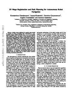
NBS, which is selected from a stack of scan paths viewing holes. BH/IG achieves a higher object coverage than S/IG in every case. After 5 scans, for S/IG part of the head and statue base are missing. The table shows that BH/IG can achieve a high object coverage co very quickly. It reaches a co of 97.9% after 10 scans which the S/IG does not even accomplish after 30 scans. The reason for this is that scan paths of BH/IG are based on boundaries and holes and these are determined based on the contour and coverage of the acquired surface model, whereas the paths of S/IG are very general and not adapted to the scan data. After 15 scans, the meshes do not change much. The final mesh of S/IG has a larger hole in the base area and a few holes on the back side. The triangle mesh of the BH/IG method after 30 scans, contains only two small holes which are not visible in figure 3, but apart from that is complete. These results show that by using a local method to determine possible scan path candidates, the completeness of the resulting 3D model can be improved in comparison to applying a sphere search space. C. Real Experiments
Fig. 3. The object coverage of the triangle meshes of the putto statue after 5, 15 and 30 scans (from left to right) are shown for S/IG (top) and BH/IG (bottom). BH/IG completes the mesh a lot better and contains less holes in each case.
The resulting triangle meshes after 5, 15 and 30 scans can be seen in figure 3. For BH/IG, after scan number 8, holes in the mesh are detected and all further scans are based on a
The performance of our suggested autonomous 3D modeling method BH/IG, which proved to generate the best model results when compared to other methods, is evaluated on a Kuka KR16 industrial robot and in a real environment (see subsection IV-A). The putto statue is located on a small table, which allows for viewing the object from several positions around the object. However, not all scan paths could be reached. The total time for 3D modeling of the putto statue was approx. 25 minutes, which is comparable to the time it would take a human to scan the object. This includes the time for moving the robot while scanning, updating the voxelspace, selecting a NBS, determining a collision free path and moving the robot to the start pose of the NBS. Moving the robot and updating the space required most of the time. During scanning, the robot was moved slowly on purpose, in order to obtain a high point density. In future, the space update can be further optimized by parallelization. The system terminated after 23 scans. Figure 4 shows the resulting mesh, which consists of 138887 triangles, and voxelspace, which was updated with Bayes’ Rule. The average edge length of the mesh was 3mm, which corresponds to the voxelspace, which has a resolution of 5mm. Black voxels in the figure refer to the state “free”, whereas white refers to “occupied”. The voxelspace does not contain any holes, whereas the mesh consists of a few smaller holes in the region of the arms and legs. The holes remain due to the workspace of the robot and the sensor characteristics. The ground truth, which was used during the simulation, is registered and compared with the generated mesh, in order to evaluate the model quality. The object coverage co was 96.8% and the coordinate root mean square error was 1.72mm. These first results of our autonomous 3D modeling system, are promising concerning model quality and acquisition time.
problem, we will perform a better adaption of the scan path to surface trend normals. This could be realized by a spline trajectory of the robot, which moves along the object contour. VI. ACKNOWLEDGMENTS Our special thanks go to Daniel Seth for his support with the dynamic octree and to Andreas D¨omel for his help with the implementation of the collision free path planner. R EFERENCES
Fig. 4. The resulting triangle mesh and voxelspace were generated with a laser stripe profiler attached to an industrial robot . The mesh contains a few small holes (red marks) but still has a high object coverage of 96.8%.
V. CONCLUSIONS AND FUTURE WORK We have presented an autonomous 3D object modeling system, which iteratively searches for possible scan paths in the local surface model and selects a next-best-scan (NBS) in the volumetric model. We focus on maximizing the quality of the 3D model instead of minimizing the number of views. Our system explores the unknown environment and simultaneously generates a 3D model of an unknown object with a desired surface completeness, which is an estimate of the actual object coverage. A probabilistic octree is used to select a NBS with the highest expected information gain and also to avoid collisions in the robot workspace. The implementation is compared with other NBV approaches and evaluated on an industrial robot with a laser stripe profiler. Our local search method, which allows for a 6DOF search space, is compared to a global sphere search space (2DOF), which is often used in NBV approaches. The results show that for objects with complex geometry or occlusions, a local scan path search improves the performance and mesh quality in comparison to simply initializing a sphere search space. Furthermore, a 3D surface model with high quality is autonomously generated on the robot. Currently the NBS is selected with the aim to maximize information to reduce unknown area. In future, we want to improve the quality of the previously scanned areas, which lack a sufficient point density or completeness. Therefore, adequate quality factors, which represent the actual quality of the surface model, could be used to select a NBS, in addition to the IG measure. This would ensure that the workspace is explored but also the information of the previously scanned data is improved. Furthermore, due to the linear scan paths, many occlusions occur and the angle between measurement beam and surface normal is often not optimal. This leads to a model of improvable quality. In order to cope with this
[1] J. Maver and R. Bajcsy, “Occlusions as a Guide for Planning the Next View,” IEEE PAMI, vol. 15, pp. 417–433, 1993. [2] R. Pito, “A Solution to the Next Best View Problem for Automated Surface Acquisition,” IEEE PAMI, vol. 21, no. 10, pp. 1016–1030, 1999. [3] W. R. Scott, G. Roth, and J.-F. Rivest, “View Planning for Automated 3D Object Reconstruction Inspection,” ACM Comput. Surv., vol. 35, no. 1, pp. 64–96, 2003. [4] S. Chen, Y. Li, and N. M. Kwok, “Active vision in robotic systems: A survey of recent developments,” I. J. Robotic Res., vol. 30, no. 11, pp. 1343–1377, 2011. [5] P. Blaer and P. K. Allen, “Data acquisition and view planning for 3-d modeling tasks,” in IEEE/RSJ IROS, San Diego, California, USA, Oct. 2007, pp. 417–422. [6] L. M. Wong, C. Dumont, and M. A. Abidi, “Next Best View System in a 3-D Object Modeling Task,” in IEEE CIRA, Monterey, California, Nov. 1999, pp. 306–311. [7] M. Trummer, C. Munkelt, and J. Denzler, “Online Next-Best-View Planning for Accuracy Optimization Using an Extended E-Criterion,” in IEEE ICPR, Istanbul, Turkey, Aug. 2010, pp. 1642–1645. [8] M. Callieri, A. Fasano, G. Impoco, P. Cignoni, R. Scopigno, G. Parrini, and G. Biagini, “RoboScan: An Automatic System for Accurate and Unattended 3D Scanning,” in IEEE 3DPVT, Thessaloniki, Greece, Sept. 2004, pp. 805–812. [9] S. Larsson and J. A. P. Kjellander, “Path planning for laser scanning with an industrial robot,” RAS, vol. 56, no. 7, pp. 615–624, 2008. [10] M. Levoy, K. Pulli, B. Curless, S. Rusinkiewicz, D. Koller, L. Pereira, M. Ginzton, S. Anderson, J. Davis, J. Ginsberg, J. Shade, and D. Fulk, “The digital michelangelo project: 3D scanning of large statues,” in SIGGRAPH, July 2000, pp. 131–144. [11] T. Bodenm¨uller, “Streaming Surface Reconstruction from Real Time 3D Measurements,” Ph.D. dissertation, Technische Universit¨at M¨unchen (TUM), 2009. [12] S. Y. Chen and Y. Li, “Vision sensor planning for 3-d model acquisition,” IEEE TSMC, vol. 35, no. 5, pp. 894–904, 2005. [13] S. Kriegel, T. Bodenm¨uller, M. Suppa, and G. Hirzinger, “A SurfaceBased Next-Best-View Approach for Automated 3D Model Completion of Unknown Objects,” in IEEE ICRA, Shanghai, China, May 2011, pp. 4869–4874. [14] L. Torabi and K. Gupta, “An autonomous six-DOF eye-in-hand system for in situ 3D object modeling,” I. J. Robotic Res., vol. 31, no. 1, pp. 82–100, 2012. [15] M. Suppa, “Autonomous Robot Work Cell Exploration using Multisensory Eye-in-Hand Systems,” Ph.D. dissertation, Leibniz Universit¨at Hannover, 2008. [16] B. Loriot, S. Ralph, and P. Gorria, “Non-Model Based Method for an Automation of 3D Acquisition and Post-Processing,” ELCVIA, vol. 7, no. 3, pp. 67–82, 2008. [17] S. Thrun, W. Burgard, and D. Fox, Probabilistic Robotics. MA: MIT Press, 2005. [18] J. J. Kuffner and S. M. LaValle, “RRT-Connect: An Efficient Approach to Single-Query Path Planning,” in IEEE ICRA, San Francisco, CA, USA, Apr. 2000, pp. 781–787. [19] L. E. Kavraki, P. Svestka, J.-C. Latombe, and M. K. Overmars, “Probabilistic roadmaps for path planning in high-dimensional configuration spaces,” IEEE Trans. on Robotics and Automation, vol. 12, no. 4, pp. 566–580, 1996. [20] M. Suppa, S. Kielh¨ofer, J. Langwald, F. Hacker, K. H. Strobl, and G. Hirzinger, “The 3D-Modeller: A Multi-Purpose Vision Platform,” in IEEE ICRA, Roma, Italy, Apr. 2007, pp. 781–787. [21] C. Munkelt, M. Trummer, S. Wenhardt, and J. Denzler, “Benchmarking 3D Reconstructions from Next Best View Planning,” MVA, pp. 552– 555, 2007.