A survey of top-k query processing techniques in relational database ...

A Survey of Top-k Query Processing Techniques in Relational Database Systems IHAB F. ILYAS, GEORGE BESKALES and MOHAMED A. SOLIMAN David R. Cheriton School of Computer Science University of Waterloo Efficient processing of top-k queries is a crucial requirement in many interactive environments that involve massive amounts of data. In particular, efficient top-k processing in domains such as the Web, multimedia search and distributed systems has shown a great impact on performance. In this survey, we describe and classify top-k processing techniques in relational databases. We discuss different design dimensions in the current techniques including query models, data access methods, implementation levels, data and query certainty, and supported scoring functions. We show the implications of each dimension on the design of the underlying techniques. We also discuss top-k queries in XML domain, and show their connections to relational approaches. Categories and Subject Descriptors: H.2.4 [Database Management]: Systems General Terms: Algorithms, Design, Experimentation, Performance Additional Key Words and Phrases: top-k, rank-aware processing, rank aggregation, voting

1. INTRODUCTION Information systems of different types use various techniques to rank query answers. In many application domains, end-users are more interested in the most important (top-k) query answers in the potentially huge answer space. Different emerging applications warrant efficient support for top-k queries. For instance, in the context of the Web, the effectiveness and efficiency of meta-search engines, which combine rankings from different search engines, are highly related to efficient rank aggregation methods. Similar applications exist in the context of information retrieval [Salton and McGill 1983] and data mining [Getoor and Diehl 2005]. Most of these applications compute queries that involve joining and aggregating multiple inputs to provide users with the top-k results. One common way to identify the top-k objects is scoring all objects based on some scoring function. An object score acts as a valuation for that object according to its characteristics (e.g., price and size of house objects in a real estate database, or color and texture of images in a multimedia database). Data objects are usually evaluated by multiple scoring predicates that contribute to the total object score. A scoring function is therefore usually defined as an aggregation over partial scores. Authors Address: University of Waterloo, 200 University Ave. West, Waterloo, Ontario, Canada N2L 3G1; email: ilyas,gbeskale,[email protected] Support was provided in part by the Natural Sciences and Engineering Research Council of Canada through Grant 311671-05 Permission to make digital/hard copy of all or part of this material without fee for personal or classroom use provided that the copies are not made or distributed for profit or commercial advantage, the ACM copyright/server notice, the title of the publication, and its date appear, and notice is given that copying is by permission of the ACM, Inc. To copy otherwise, to republish, to post on servers, or to redistribute to lists requires prior specific permission and/or a fee. c 20YY ACM 0000-0000/20YY/0000-0001 $5.00 ° ACM Journal Name, Vol. V, No. N, Month 20YY, Pages 1–61.

·

2

HID 1 2 3 4 5 6

Ilyas et al.

Location Lafayette W.Lafayette Indianapolis Kokomo Lafayette Kokomo

……

Price

SID

Location

Tuition

90,000 110,000 111,000 118,000 125,000 154,000

1 2 3 4 5 6 7 8

Indianapolis W.Lafayette Lafayette Lafayette Indianapolis Indianapolis Kokomo Kokomo

3000 3500 6000 6200 7000 7900 8200 8200

HID

SID

Price + 10 x Tuition

1

3

150000

1

4

152000

2

2

145000

3

1

141000

Join Result

Schools

Houses Fig. 1.

A Top-k Query Example

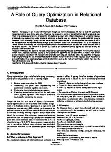
Top-k processing connects to many database research areas including query optimization, indexing methods and query languages. As a consequence, the impact of efficient top-k processing is becoming evident in an increasing number of applications. The following examples illustrate real-world scenarios where efficient top-k processing is crucial. The examples highlight the importance of adopting efficient top-k processing techniques in traditional database environments. E XAMPLE 1.1. Consider a user interested in finding a location (e.g., city) where the combined cost of buying a house and paying school tuition for 10 years at that location is minimum. The user is interested in the five least expensive places. Assume that there are two external sources (databases), Houses and Schools, that can provide information on houses and schools, respectively. The Houses database provides a ranked list of the cheapest houses and their locations. Similarly, the Schools database provides a ranked list of the least expensive schools and their locations. Figure 1 gives an example of the Houses and Schools databases. A na¨ıve way to answer the query described in Example 1.1 is to retrieve two lists: A list of the cheapest houses from Houses, and a list of the cheapest schools from Schools. These two lists are then joined based on location such that a valid join result is comprised of a house and a school at the same location. For all join results, the total cost of each houseschool pair is computed, for example, by adding the house price and the school tuition for ten years. The five cheapest pairs constitute the final answer to this query. Figure 1 shows an illustration for the join process between houses and schools lists, and partial join results. Note that the top five results cannot be returned to the user until all the join results are generated. For large numbers of co-located houses and schools, the processing of such query, in the traditional manner, is very expensive as it requires expensive join and sort operations for large amounts of data. E XAMPLE 1.2. Consider a video database system where several visual features are extracted from each video object (frame or segment). Example features include color histograms, color layout, texture, and edge orientation. Features are stored in separate relations indexed using high-dimensional indexes that support similarity queries. Suppose that ACM Journal Name, Vol. V, No. N, Month 20YY.

A Survey of Top-k Query Processing Techniques in Relational Database Systems

·

3

Query Color Histogram

Edge Histogram

Texture

Video Database

Color Histogram Edge Histogram Texture

Fig. 2.

Single and Multi-feature Queries in Video Database

a user is interested in the top 10 video frames most similar to a given query image based on a set of visual features. Example 1.2 draws attention to the importance of efficient top-k processing in similarity queries. In video databases [Aref et al. 2004], hours of video data are stored inside the database producing huge amounts of data. Top-k similarity queries are traditionally answered using high-dimensional indexes built on individual video features, and a nearestneighbor scan operator on top of these indexes. A database system that supports approximate matching ranks objects depending on how well they match the query example. Figure 2 presents an example of single-feature similarity query based on color histogram, texture and edge orientation. More useful similarity queries could involve multiple features. For example, suppose that a user is interested in the top 10 video frames most similar to a given query image based on color and texture combined. User could provide a function that combines similarity scores in both features into an overall similarity score. For example, the global score of a frame f with respect to a query image q could be computed as: 0.5 × ColorSimilarity(f, q) + 0.5 × T extureSimilarity(f, q). One way to answer such multi-feature query is by sequentially scanning all database objects, computing the score of each object according to each feature, and combining the scores into a total score for each object. This approach suffers from scalability problems with respect to database size and the number of features. An alternative way is to map the query into a join query that joins the output of multiple single-feature queries, and then sorts the joined results based on combined score. This approach also does not scale with respect to both number of features and database size since all join results have to be computed then sorted. The main problem with sort-based approaches is that sorting is a blocking operation that requires full computation of the join results. Although the input to the join operation is sorted on individual features, this order is not exploited by conventional join algorithms. Hence, sorting the join results becomes necessary to produce the top-k answers. Embedding rank-awareness in query processing techniques provides a more efficient and scalable solution. In this survey, we discuss the state-of-the-art top-k query processing techniques in reACM Journal Name, Vol. V, No. N, Month 20YY.

4

·

Ilyas et al.

Notation m Li t or o g F F (t) or F (o) F (t) or F (o) pi (t) or pi (o) pmax i pmin i pi T Ak Mk

Description Number of sources (lists) Ranked source (list) number i A tuple or object to be scored A group of tuples based on some grouping attributes Scoring (ranking) Function Score lower bound of t (or o) Score upper bound of t (or o) The value of scoring predicate pi applied to t (or o). Predicate pi determines objects order in Li The maximum score of predicate pi The minimum score of predicate pi The score upper bound of predicate pi (mostly refers to the score of the last seen object in Li ) Score threshold (cutoff value) The current top-k set The minimum score in the current top-k set Table I.

Frequently Used Notations

lational database systems. We give a detailed coverage for most of the recently presented techniques focusing primarily on their integration into relational database environments. We also introduce a taxonomy to classify top-k query processing techniques based on multiple design dimensions, described in the following: —Query Model: Top-k processing techniques are classified according to the query model they assume. Some techniques assume a selection query model, where scores are attached directly to base tuples. Other techniques assume a join query model, where scores are computed over join results. A third category assumes an aggregate query model, where we are interested in ranking groups of tuples. —Data Access Methods: Top-k processing techniques are classified according to the data access methods they assume to be available in the underlying data sources. For example, some techniques assume the availability of random access, while others are restricted to only sorted access. —Implementation Level: Top-k processing techniques are classified according to their level of integration with database systems. For example, some techniques are implemented in an application layer on top of the database system, while others are implemented as query operators. —Data and Query Uncertainty: Top-k processing techniques are classified based on the uncertainty involved in their data and query models. Some techniques produce exact answers, while others allow for approximate answers, or deal with uncertain data. —Ranking Function: Top-k processing techniques are classified based on the restrictions they impose on the underlying ranking (scoring) function. Most proposed techniques assume monotone scoring functions. Few proposals address general functions. Notations. The working environments, of most of the techniques we describe, assume a scoring (ranking) function used to score objects (tuples) by aggregating the values of their partial scores (scoring predicates). Table I lists the frequently used notations in this survey.

ACM Journal Name, Vol. V, No. N, Month 20YY.


·

5

Top-k Processing Techniques

Query Model Top-k Selection

Data & Query Certainty

Top-k Aggregate

Top-k Join

Data Access

No Random

Implementation Level Ranking Function

Sorted + Controlled Random Probes

Monotone Unspecified

Both Sorted and Random

Certain Data, Exact Methods

Uncertain Data

Generic

Query Engine

Application Level

Certain Data, Approximate Methods

Indexes / Materialized Views

Filter-Restart

Fig. 3. Classification of Top-k Query Processing Techniques

Outline. The remainder of this survey is organized as follows. Section 2 introduces the taxonomy we adopt in this survey to classify top-k query processing methods. Sections 3, 4, 5 and 6 discuss the different design dimensions of top-k processing techniques, and give the details of multiple techniques in each dimension. Section 7 discusses related top-k processing techniques for XML data. Section 8 presents related background from voting theory, which forms the basis of many current top-k processing techniques. Section 9 concludes this survey, and describes future research directions. We assume the reader of this survey has a general familiarity with relational database concepts. 2. TAXONOMY OF TOP-K QUERY PROCESSING TECHNIQUES Supporting efficient top-k processing in database systems is a relatively recent and active line of research. Top-k processing has been addressed from different perspectives in the current literature. Figure 3 depicts the classification we adopt in this survey to categorize different top-k processing techniques based on their capabilities and assumptions. In the following sections, we discuss our classification dimensions, and their impact on the design of the underlying top-k processing techniques. For each dimension, we give a detailed description for one or more example techniques. 2.1 Query Model Dimension Current top-k processing techniques adopt different query models to specify the data objects to be scored. We discuss three different models: (1) top-k selection query, (2) top-k join query, and (3) top-k aggregate query. We formally define these query models in the following. ACM Journal Name, Vol. V, No. N, Month 20YY.

6

·

Ilyas et al.

2.1.1 Top-k Selection Query Model. In this model, the scores are assumed to be attached to base tuples. A top-k selection query is required to report the k tuples with the highest scores. Scores might not be readily available since they could be the outcome of some user-defined scoring function that aggregates information coming from different tuple attributes. Definition 2.1. Top-k Selection Query. Consider a relation R, where each tuple in R has n attributes. Consider m scoring predicates, p1 . . . pm defined on these attributes. Let F (t) = F (p1 (t), . . . , pm (t)) be the overall score of tuple t ∈ R. A top-k selection query selects the k tuples in R with the largest F values. A SQL template for top-k selection query is the following: SELECT some attributes FROM R WHERE selection condition ORDER BY F (p1 , . . . , pm ) LIMIT k 1

Consider Example 1.2. Assume the user is interested in finding the top-10 video objects that are most similar to a given query image q, based on color and texture, and whose release date is after 1/1/2008. This query could be written as follows: SELECT v.id FROM V ideoObject v WHERE v.date > ’01/01/2008’ ORDER BY 0.5 ∗ ColorSimilarity(q, v) + 0.5 ∗ T extureSimilarity(q, v) LIMIT 10

The NRA algorithm [Fagin et al. 2001] is one example of top-k techniques that adopt the top-k selection model. The input to the NRA algorithm is a set of sorted lists, each ranks the “same” set of objects based on different attributes. The output is a ranked list of these objects ordered on the aggregate input scores. We give the full details of this algorithm in Section 3.2. 2.1.2 Top-k Join Query Model. In this model, scores are assumed to be attached to join results rather than base tuples. A top-k join query joins a set of relations based on some arbitrary join condition, assigns scores to join results based on some scoring function, and reports the top-k join results. Definition 2.2. Top-k Join Query. Consider a set of relations R1 . . . Rn . A top-k join query joins R1 . . . Rn , and returns the k join results with the largest combined scores. The combined score of each join result is computed according to some function F (p1 , . . . , pm ), where p1 , . . . , pm are scoring predicates defined over the join results. A possible SQL template for a top-k join query is: SELECT * FROM R1 , . . . , Rn WHERE join condition(R1 , . . . , Rn ) 1 Other

keywords, e.g., Stop After k, are also used in other SQL dialects.



·

7

ORDER BY F (p1 , . . . , pm ) LIMIT k

For example, the top-k join query in Example 1.1 could be formulated as follows: SELECT h.id, s.id FROM House h, School s WHERE h.location=s.location ORDER BY h.price + 10 ∗ s.tuition LIMIT 5

A top-k selection query can be formulated as a special top-k join query by partitioning R into n vertical relations R1 , . . . , Rn , such that each relation Ri has the necessary attributes to compute the score pi . For example, Let R contains the attributes tid, A1 , A2 , and A3 . Then, R can be partitioned into R1 = (tid, A1 ) and R2 = (tid, A2 , A3 ), where p1 = A1 and p2 = A2 +A3 . In this case, the join condition is an equality condition on key attributes. The NRA-RJ algorithm [Ilyas et al. 2002] is one example of top-k processing techniques that formulate top-k selection queries as top-k join queries based on tuples’ keys. Many top-k join techniques address the interaction between computing the join results and producing the top-k answers. Examples are the J* algorithm [Natsev et al. 2001] (Section 3.2), and the Rank-Join algorithm [Ilyas et al. 2004] (Section 4.2). Some techniques, e.g., PREFER [Hristidis et al. 2001] (Section 4.1.2), process top-k join queries using auxiliary structures that materialize join results, or by ranking the join results after they are generated. 2.1.3 Top-k Aggregate Query Model. In this model, scores are computed for tuple groups, rather than individual tuples. A top-k aggregate query reports the k groups with the largest scores. Group scores are computed using a group aggregate function such as sum. Definition 2.3. Top-k Aggregate Query. Consider a set of grouping attributes G={g1 , . . . , gr }, and an aggregate function F that is evaluated on each group. A top-k aggregate query returns the k groups, based on G, with the highest F values. A SQL formulation for a top-k aggregate query is : SELECT g1 , . . . , gr , F FROM R1 , . . . , Rn WHERE join condition(R1 , . . . , Rn ) GROUP BY g1 , . . . , gr ORDER BY F LIMIT k

An example top-k aggregate query is to find the best five areas to advertise student insurance product, based on the score of each area, which is a function of student’s income, age and credit. SELECT S.zipcode,Average(income*w1 + age*w2 + credit*w3) as score FROM customer WHERE occupation = ’student’ GROUP BY zipcode ACM Journal Name, Vol. V, No. N, Month 20YY.

8

·

Ilyas et al.

ORDER BY score LIMIT 5

Top-k aggregate queries add additional challenges to top-k join queries: (1) interaction of grouping, joining, and scoring of query results, and (2) non-trivial estimation of the scores of candidate top-k groups. A few recent techniques, e.g., [Li et al. 2006], address these challenges to efficiently compute top-k aggregate queries. We discuss these techniques in Section 4.2. 2.2 Data Access Dimension Many top-k processing techniques involve accessing multiple data sources with different valuations of the underlying data objects. A typical example is a meta-searcher that aggregates the rankings of search hits produced by different search engines. The hits produced by each search engine can be seen as a ranked list of web pages based on some score, e.g., relevance to query keywords. The manner in which these lists are accessed largely affects the design of the underlying top-k processing techniques. For example, ranked lists could be scanned sequentially in score order. We refer to this access method as sorted access. Sorted access is supported by a DBMS if, for example, a B-Tree index is built on objects’ scores. In this case, scanning the sequence set (leaf level) of the B-Tree index provides a sorted access of objects based on their scores. On the other hand, the score of some object might be required directly without traversing the objects with higher/smaller scores. We refer to this access method as random access. Random access could be provided through index lookup operations if an index is built on object keys. We classify top-k processing techniques, based on the assumptions they make about available data access methods in the underlying data sources, as follows: —Both Sorted and Random Access: In this category, top-k processing techniques assume the availability of both sorted and random access in all the underlying data sources. Examples are TA [Fagin et al. 2001], and the Quick-Combine algorithm [Güntzer et al. 2000]. We discuss the details of these techniques in Section 3.1. —No Random Access: In this category, top-k processing techniques assume the underlying sources provide only sorted access to data objects based on their scores. Examples are the NRA algorithm [Fagin et al. 2001], and the Stream-Combine algorithm [Güntzer et al. 2001]. We discuss the details of these techniques in Section 3.2. —Sorted Access with Controlled Random Probes: In this category, top-k processing techniques assume the availability of at least one sorted access source. Random accesses are used in a controlled manner to reveal the overall scores of candidate answers. Examples are the Rank-Join algorithm [Ilyas et al. 2004], the MPro algorithm [Chang and Hwang 2002], and the Upper and Pick algorithms [Bruno et al. 2002]. We discuss the details of these techniques in Section 3.3. 2.3 Implementation Level Dimension Integrating top-k processing with database systems is addressed in different ways by current techniques. One approach is to embed top-k processing in an outer layer on-top of the database engine. This approach allows for easy extensibility of top-k techniques, since they are decoupled from query engines. The capabilities of database engines (e.g., storage, indexing and query processing) are leveraged to allow for efficient top-k processing. ACM Journal Name, Vol. V, No. N, Month 20YY.


·

9

New data access methods or specialized data structures could also be built to support top-k processing. However, the core of query engines remains unchanged. Another approach is to modify the core of query engines to recognize the ranking requirements of top-k queries during query planning and execution. This approach has a direct impact on query processing and optimization. Specifically, query operators are modified to be rank-aware. For example, a join operator is required to produce ranked join results to support pipelining top-k query answers. Moreover, available access methods for ranking predicates are taken into account while optimizing a query plan. We classify top-k processing techniques based on their level of integration with database engines as follows: —Application Level: This category includes top-k processing techniques that work outside the database engine. Some of the techniques in this category rely on the support of specialized top-k indexes or materialized views. However, the main top-k processing remains outside the engine. Examples are [Chang et al. 2000], and [Hristidis et al. 2001]. Another group of techniques formulate top-k queries as range queries that are repeatedly executed until the top-k objects are obtained. We refer to this group of techniques as Filter-Restart. One example is [Donjerkovic and Ramakrishnan 1999]. We discuss the details of these techniques in Section 4.1. —Query Engine Level: This category includes techniques that involve modifications to the query engine to allow for rank-aware processing and optimization. Some of these techniques introduce new query operators to support efficient top-k processing. For example, [Ilyas et al. 2004] introduce rank-aware join operators. Other techniques, e.g., [Li et al. 2005; Li et al. 2006], extend rank-awareness to query algebra to allow for extensive query optimization. We discuss the details of these techniques in Section 4.2. 2.4 Query and Data Uncertainty Dimension In some query processing environments, e.g., decision support or OLAP, obtaining exact query answers efficiently may be overwhelming to database engine because of the interactive nature of such environments, and the sheer amounts of data they usually handle. Such environments could sacrifice the accuracy of query answers in favor of performance. In these settings, it may be acceptable for a top-k query to report approximate answers. The uncertainty in top-k query answers might alternatively arise due to the nature of the underlying data itself. Applications in domains such as sensor networks, data cleaning, and moving objects tracking involve processing data that is probabilistic in nature. For example, the temperature reading of some sensor could be represented as a probability distribution over a continuous interval, or a customer name in a dirty database could be a represented as a set of possible names. In these settings, top-k queries, as well as other query types, need to be formulated and processed while taking data uncertainty into account. We classify top-k processing techniques based on query and data certainty as follows: —Exact Methods over Certain Data: This category includes the majority of current top-k processing techniques, where deterministic top-k queries are processed over deterministic data. —Approximate Methods over Certain Data: This category includes top-k processing techniques that operate on deterministic data, but report approximate answers in favor of ACM Journal Name, Vol. V, No. N, Month 20YY.

10

·

Ilyas et al.

performance. The approximate answers are usually associated with probabilistic guarantees indicating how far they are from the exact answer. Examples include [Theobald et al. 2005] and [Amato et al. 2003]. We discuss the details of these techniques in Section 5.1. —Uncertain Data: This category includes top-k processing techniques that work on probabilistic data. The research proposals in this category formulate top-k queries based on different uncertainty models. Some approaches treat probabilities as the only scoring dimension, where a top-k query is a Boolean query that reports the k most probable query answers. Other approaches study the interplay between the scoring and probability dimensions. Examples are [Ré et al. 2007] and [Soliman et al. 2007]. We discuss the details of these techniques in Section 5.2. 2.5 Ranking Function Dimension The properties of the ranking function largely influence the design of top-k processing techniques. One important property is the ability to upper bound objects’ scores. This property allows early pruning of certain objects without exactly knowing their scores. A monotone ranking function can largely facilitate upper bound computation. A function F , defined on predicates p1 , . . . , pn , is monotone if F (p1 , . . . , pn ) ≤ F (p´1 , . . . , pń ) whenever pi ≤ pí for every i. We elaborate on the impact of function monotonicity on top-k processing in Section 6.1. In more complex applications, a ranking function might need to be expressed as a numeric expression to be optimized. In this setting, the monotonicity restriction of the ranking function is relaxed to allow for more generic functions. Numerical optimization tools as well as indexes are used to overcome the processing challenges imposed by such ranking functions. Another group of applications address ranking objects without specifying a ranking function. In some environments, such as data exploration or decision making, it might not be important to rank objects based on a specific ranking function. Instead, objects with high quality based on different data attributes need to be reported for further analysis. These objects could possibly be among the top-k objects of some unspecified ranking function. The set of objects that are not dominated by any other objects, based on some given attributes, are usually referred to as the skyline. We classify top-k processing techniques based on the restrictions they impose on the underlying ranking function as follows: —Monotone Ranking Function: Most of the current top-k processing techniques assume monotone ranking functions since they fit in many practical scenarios, and have appealing properties allowing for efficient top-k processing. One example is [Fagin et al. 2001]. We discuss the properties of monotone ranking functions in Section 6.1. —Generic Ranking Function: Few recent techniques, e.g., [Zhang et al. 2006], address top-k queries in the context of constrained function optimization. The ranking function in this case is allowed to take a generic form. We discuss the details of these techniques in Section 6.2. —No Ranking Function: Many techniques have been proposed to answer skyline related queries, e.g., [Börzsönyi et al. 2001] and [Yuan et al. 2005]. Covering current skyline literature in details is out of the scope of this survey. We believe it worths a dedicated ACM Journal Name, Vol. V, No. N, Month 20YY.


·

11

survey by itself. However, we briefly show the connection between skyline and top-k queries in Section 6.3. 2.6 Impact of Design Dimensions on Top-k Processing Techniques Figure 4 shows the properties of a sample of different top-k processing techniques that we describe in this survey. The applicable categories under each taxonomy dimension are marked for each technique. For example, TA [Fagin et al. 2001] is an exact method that assumes top-k selection query model, and operates on certain data, exploiting both sorted and random access methods. TA integrates with database systems at the application level, and supports monotone ranking functions. Our taxonomy encapsulates different perspectives to understand the processing requirements of current top-k processing techniques. The taxonomy dimensions, discussed in the previous sections, can be viewed as design dimensions that impact the capabilities and the assumptions of the underlying top-k algorithms. In the following, we give some examples of the impact of each design dimension on the underlying top-k processing techniques: —Impact of Query Model: The query model significantly affects the solution space of the top-k algorithms. For example, the top-k join query model (Definition 2.2) imposes tight integration with the query engine and physical join operators to efficiently navigate the Cartesian space of join results. —Impact of Data Access: Available access methods affect how different algorithms compute bounds on object scores and hence affect the termination condition. For example, the NRA algorithm [Fagin et al. 2001], discussed in Section 3.2, has to compute “range” of possible scores for each object since the lack of random access prevents computing an exact score for each seen object. On the other hand, allowing random access to the underlying data sources triggers the need for cost models to optimize the number of random and sorted accesses. One example is the CA algorithm [Fagin et al. 2001], discussed in Section 3.1. —Impact of Data and Query Uncertainty: Supporting approximate query answers requires building probabilistic models to fit the score distributions of the underlying data, as proposed in [Theobald et al. 2004] (Section 5.1.2). Uncertainty in the underlying data adds further significant computational complexity because of the huge space of possible answers that needs to be explored. Building efficient search algorithms to explore such space is crucial, as addressed in [Soliman et al. 2007]. —Impact of Implementation Level: The implementation level greatly affects the requirements of the top-k algorithm. For example, implementing top-k pipelined query operator necessitates using algorithms that require no random access to their inputs to fit in pipelined query models, it also requires the output of the top-k algorithm to be a valid input to another instance of the algorithm [Ilyas et al. 2004]. On the other hand, implementation on the application level does not have these requirements. More details are given in Section 4.2.1. —Impact of Ranking Function: Assuming monotone ranking functions allows top-k processing techniques to benefit from the monotonicity property to guarantee early-out of query answers. Dealing with non-monotone functions requires more sophisticated bounding for the scores of unexplored answers. Existing indexes in the database are currently used to provide such bounding, as addressed in [Xin et al. 2007] (Section 6). ACM Journal Name, Vol. V, No. N, Month 20YY.

12

·

Ilyas et al.

Query Model

9

Rank-Join (Ilyas et al. 2003) RankSQL - ȝ operator (Li 2005)

9 9

rankaggr Operator (Li 2006) KLEE (Michel et al. 2005)

9

OPTU-Topk (Soliman et al. 2007)

9 9

MS_Topk (Ré et al. 2007)

Fig. 4.

9

9

9

9

9

9 9 9 9 9

9 9 9 9 9

9

9

9 9 N/A 9 9 9 9

9 9

OPT* (Zhang et al. 2006)

9

9 9

9 9 9 9

9 9

TopX (Theobald et al. 2005)

9

9

9

9

NRA-RJ (Ilyas et al. 2002)

9

9

9 9 9 9

N/A

9 9 9

9 9 N/A 9

9 9

9

Generic

9

Monotone

PREFER (Hristidis et al. 2001), Filter-Restart (Bruno et al. 2002), Onion Indices (Chang et al. 2000), LPTA(Das et al. 2006)

9

9

9

Application Level

J* e-approx. (Natsev et al. 2001)

Implement. Ranking Level Function

Query Engine Level

9 9

J* (Natsev et al. 2001)

Sorted + Controlled Random Probes

9 9 9 9

Both Sorted and Random

9

9 9 9

Mpro (Chang et al. 2002)

No Random

9 9

Upper/Pick (Bruno et al. 2002)

Data Access

9

NRA (Fagin et al. 2001), 9 Stream-Combine(Güntzer et al. 2001) CA (Fgain et al. 2001)

Uncertain Data

TA-Ԧ approx (Fagin et al. 2003)

Certain Data, Approx. Methods Certain Data, Exact Methods

Top-k Aggregate

Top-k Join

Top-k Selection TA (Fagin et al. 2001), 9 Quick-Combine (Güntzer et al. 2000)

Data & Query Certainty

9 9 9 9 9 9 9 9 9

Properties of Different top-k Processing Techniques

3. DATA ACCESS In this section, we discuss top-k processing techniques that make different assumptions about available access methods supported by data sources. The primary data access methods are sorted access, random access, and a combination of both methods. In sorted access, objects are accessed sequentially ordered by some scoring predicate, while for random access, objects are directly accessed by their identifiers. The techniques presented in this section assume multiple lists (possibly located at separate sources) that rank the same set of objects based on different scoring predicates. A score aggregation function is used to aggregate partial objects’ scores, obtained from the ACM Journal Name, Vol. V, No. N, Month 20YY.


·

13

Algorithm 1 TA [Fagin et al. 2001] (1) Do sorted access in parallel to each of the m sorted lists Li . As a new object o is seen under sorted access in some list, do random access to the other lists to find pi (o) in every other list Li . Compute the score F (o) = F (p1 , . . . , pm ) of object o. If this score is among the k highest scores seen so far, then remember object o and its score F (o) (ties are broken arbitrarily, so that only k objects and their scores are remembered at any time). (2) For each list Li , let pi be the score of the last object seen under sorted access. Define the threshold value T to be F (p1 , . . . , pm ). As soon as at least k objects have been seen with scores at least equal to T , halt. (3) Let Ak be a set containing the k seen objects with the highest scores. The output is the sorted set {(o, F (o))|o ∈ Ak }. different lists, to find the top-k answers. The cost of executing a top-k query, in such environments, is largely influenced by the supported data access methods. For example, random access is generally more expensive than sorted access. A common assumption in all of the techniques discussed in this section is the existence of at least one source that supports sorted access. We categorize top-k processing techniques, according to the assumed source capabilities, into the three categories described in the next sections. 3.1 Both Sorted and Random Access Top-k processing techniques in this category assume data sources that support both access methods, sorted and random. Random access allows for obtaining the overall score of some object right after it appears in one of the data sources. The Threshold Algorithm (TA) and Combined Algorithm (CA) [Fagin et al. 2001] belong to this category. Algorithm 1 describes the details of TA. The algorithm scans multiple lists, representing different rankings of the same set of objects. An upper bound T is maintained for the overall score of unseen objects. The upper bound is computed by applying the scoring function to the partial scores of the last seen objects in different lists. Notice that the last seen objects in different lists could be different. The upper bound is updated every time a new object appears in one of the lists. The overall score of some seen object is computed by applying the scoring function to object’s partial scores, obtained from different lists. To obtain such partial scores, each newly seen object in one of the lists is looked up in all other lists, and its scores are aggregated using the scoring function to obtain the overall score. All objects with total scores that are greater than or equal to T can be reported. The algorithm terminates after returning the k th output. Example 3.1 illustrates the processing of TA. E XAMPLE 3.1. TA Example: Consider two data sources L1 and L2 holding different rankings for the same set of objects based on two different scoring predicates p1 and p2 , respectively. Each of p1 and p2 produces score values in the range [0,50]. Assume each source supports sorted and random access to their ranked lists. Consider a score aggregation function F = p1 + p2 . Figure 5 depicts the first two steps of TA. In the first step, retrieving the top object from each list, and probing the value of its other scoring predicate in the other list, result in revealing the exact scores for the top objects. The seen objects ACM Journal Name, Vol. V, No. N, Month 20YY.

14

·

Ilyas et al.

First Step OID

P1 50 35 30 20 10

5 1 3 2 4

OID

P2 50 40 30 20 10

3 2 1 4 5

Second Step

T = 100 3:3:(80) (80) 5:5:(60) (60)

T = 75

OID

P1 50 35 30 20 10

5 1 3 2 4

L2

OID

P2 50 40 30 20 10

3 2 1 4 5

L1 Fig. 5.

3:3:(80) (80) 1:5:(65) (60) 5: (60) 2: (60)

Buffer

The Threshold Algorithm (TA)

are buffered in the order of their scores. A threshold value, T , for the scores of unseen objects is computed by applying F to the last seen scores in both lists, which results in 50+50=100. Since both seen objects have scores less than T , no results can be reported. In the second step, T drops to 75, and object 3 can be safely reported since its score is above T . The algorithm continues until k objects are reported, or sources are exhausted. TA assumes that the costs of different access methods are the same. In addition, TA does not have a restriction on the number of random accesses to be performed. Every sorted access in TA results in up to m-1 random accesses, where m is the number of lists. Such a large number of random accesses might be very expensive. The CA algorithm [Fagin et al. 2001] alternatively assumes that the costs of different access methods are different. The CA algorithm defines a ratio between the costs of the two access methods to control the number of random accesses, since they usually have higher costs than sorted accesses. The CA algorithm periodically performs random accesses to collect unknown partial scores for objects with the highest score lower bounds (ties are broken using score upper bounds). A score lower bound is computed by applying the scoring function to object’s known partial scores, and the worst possible unknown partial scores. On the other hand, a score upper bound is computed by applying the scoring function to object’s known partial scores, and the best possible unknown partial scores. The worst unknown partial scores are the lowest values in the score range, while the best unknown partial scores are the last seen scores in different lists. One random access is performed periodically every ∆ sorted accesses, where ∆ is the floor of the ratio between random access cost and sorted access cost. Although CA minimizes the number of random accesses compared to TA, it assumes that all sources support random access at the same cost, which may not be true in practice. This problem is addressed in [Bruno et al. 2002; Marian et al. 2004], and we discuss it in more detail in Section 3.3. ACM Journal Name, Vol. V, No. N, Month 20YY.


·

15

In TA, tuples are retrieved from sorted lists in a round-robin style. For instance, if there are m sorted access sources, tuples are retrieved from sources in this order: (L1 , L2 , . . . , Lm , L1 , . . .). Two observations can possibly minimize the number of retrieved tuples. First, sources with rapidly decreasing scores can help decrease the upper bound of unseen objects’ scores (T ) at a faster rate. Second, favoring sources with considerable influence on the overall scores could lead to identifying the top answers quickly. Based on these two observations, a variation of TA, named Quick-Combine, is introduced in [Güntzer et al. 2000]. The Quick-Combine algorithm uses an indicator ∆i expressing the effectiveness of reading from source i, defined as follows: ∆i =

∂F · (Si (di − c) − Si (di )) ∂pi

(1)

where Si (x) refers to the score of the tuple at depth x in source i, and di is the current depth reached at source i. The rate at which score decays in source i is computed as the difference between its last seen score Si (di ), and the score of the tuple c steps above in the ranked list, Si (di − c). The influence of source i on the scoring function F is captured using the partial derivative of F with respect to source’s predicate pi . The source with the maximum ∆i is selected, at each step, to get the next object. It has been shown that the proposed algorithm is particularly efficient when the data exhibits tangible skewness. 3.2 No Random Access The techniques we discuss in this section assume random access is not supported by the underlying sources. The No Random Access (NRA) algorithm [Fagin et al. 2001] and the Stream-Combine algorithm [Güntzer et al. 2001] are two examples of the techniques that belong to this category. The NRA algorithm finds the top-k answers by exploiting only sorted accesses. The NRA algorithm may not report the exact object scores, as it produces the top-k answers using bounds computed over their exact scores. The score lower bound of some object t is obtained by applying the score aggregation function on t’s known scores and the minimum possible values of t’s unknown scores. On the other hand, the score upper bound of t is obtained by applying the score aggregation function on t’s known scores and the maximum possible values of t’s unknown scores, which are the same as the last seen scores in the corresponding ranked lists. This allows the algorithm to report a top-k object even if its score is not precisely known. Specifically, if the score lower bound of an object t is not below the score upper bounds of all other objects (including unseen objects), then t can be safely reported as the next top-k object. The details of the NRA algorithm are given in Algorithm 2. Example 3.2 illustrates the processing of the NRA algorithm. E XAMPLE 3.2. NRA Example: Consider two data sources L1 and L2 , where each source holds a different ranking of the same set of objects based on scoring predicates p1 and p2 , respectively. Both p1 and p2 produce score values in the range [0,50]. Assume both sources support only sorted access to their ranked lists. Consider a score aggregation function F = p1 + p2 . Figure 6 depicts the first three steps of the NRA algorithm. In the first step, retrieving the first object in each list gives lower and upper bounds for objects’ scores. For example, object 5 has a score range of [50,100], since the value of its known scoring predicate p1 is 50, while the value of its unknown scoring predicate p2 cannot ACM Journal Name, Vol. V, No. N, Month 20YY.

16

·

Ilyas et al.

Algorithm 2 NRA [Fagin et al. 2001] (1) Let pmin , . . . , pmin be the smallest possible values in lists L1 , . . . , Lm . m 1 (2) Do sorted access in parallel to lists L1 , . . . , Lm , and at each step do the following: —Maintain the last seen predicate values p1 , . . . , pm in the m lists. —For every object o with some unknown predicate values, compute a lower bound for F (o), denoted F (o), by substituting each unknown predicate pi with pmin . Simi ilarly, Compute an upper bound F (o) by substituting each unknown predicate pi with pi . For object o that has not been seen at all, F (o) = F (pmin , . . . , pmin m ), and 1 F (o) = F (p1 , . . . , pm ). —Let Ak be the set of k objects with the largest lower bound values F (.) seen so far. If two objects have the same lower bound, then ties are broken using their upper bounds F (.), and arbitrarily among objects that additionally tie in F (.). —Let Mk be the k th largest F (.) value in Ak . (3) Call an object o viable if F (o) > Mk . Halt when (a) at least k distinct objects have been seen, and (b) there are no viable objects outside Ak . That is, if F (o) ≤ Mk for all o 6∈ Ak , return Ak . exceed 50. An upper bound for the scores of unseen objects is computed as 50+50=100, which is the result of applying F to the last seen scores in both sorted lists. The seen objects are buffered in the order of their score lower bounds. Since the score lower bound of object 5, the top buffered object, does not exceed the score upper bound of other objects, nothing can be reported. The second step adds two more objects to the buffer, and updates the score bounds of other buffered objects. In the third step, the scores of objects 1 and 3 are completely known. However, since the score lower bound of object 3 is not below the score upper bound of any other object (including the unseen ones), object 3 can be reported as the top-1 object. Note that at this step object 1 cannot be additionally reported, since the score upper bound of object 5 is 80, which is larger than the score lower bound of object 1. The Stream-Combine algorithm [Güntzer et al. 2001] is based on the same general idea of the NRA algorithm. The Stream-Combine algorithm prioritizes reading from sorted lists to give more chance to the lists that might lead to the earliest termination. To choose which sorted list (stream) to access next, an effectiveness indicator ∆i is computed for each stream i, similar to the Quick-Combine algorithm. The definition of ∆i in this case captures three properties of stream i, that may lead to early termination: (1) how rapidly scores decrease in stream i, (2) what is the influence of stream i on the total aggregated score, and (3) how many top-k objects would have their score bounds tightened by reading from stream i. The indicator ∆i is defined as follows: ∆i = #Mi ·

∂F · (Si (di − c) − Si (di )) ∂pi

(2)

where Si (x) refers to the score of the tuple at depth x in stream i, and di is the current depth reached at stream i. The term (Si (di −c)−Si (di )) captures the rate of score decay in stream i, while the term ∂F ∂pi captures how much the stream’s scoring predicate contributes to the total score, similar ACM Journal Name, Vol. V, No. N, Month 20YY.


First Step

OID

50 40 30 20 10

5 1 3 2 4

Second Step

OID

P1 50 40 30 20 10

5 1 3 2 4

Third Step

P1

OID

P1 50 40 30 20 10

5 1 3 2 4

L1

OID

OID

OID

P2 50 40 30 20 10

3 2 1 4 5

5: (50 – 100) 3: (50 – 100)

P2 50 40 30 20 10

3 2 1 4 5

17

P2 50 40 30 20 10

3 2 1 4 5

·

5: (50 – 90) 3: (50 – 90) 1: (40 – 80) 2: (40 – 80)

3: (80 – 80) 1: (70 – 70) 5: (50 – 80) 2: (40 – 70)

Buffer

L2

Fig. 6. The Three First Steps of the NRA Algorithm

to the Quick-Combine algorithm. The term #Mi is the number of top-k objects whose score bounds may be affected when reading from stream i, by reducing their score upper bounds, or knowing their precise scores. The stream with the maximum ∆i is selected, at each step, to get the next object. The NRA algorithm has been also studied in [Mamoulis et al. 2006] under various application requirements. The presented techniques rely on the observation that at some stage during NRA processing, it is not useful to keep track of up-to-date score upper bounds. Instead, the updates to these upper bounds can be deferred to a later step, or can be reduced to a much more compact set of necessary updates for more efficient computation. An NRA variant, called LARA, has been introduced based on a lattice structure that keeps a leader object for each subset of the ranked inputs. These leader objects provide score upper bounds for objects that have not been seen yet on their corresponding inputs. The top-k processing algorithm proceeds in two successive phases: —A growing phase: Ranked inputs are sequentially scanned to compose a candidate set. The seen objects in different inputs are added to the candidate set. A set Wk , containing the k objects with highest score lower bounds, is remembered at each step. The candidate set construction is complete when the threshold value (the score upper bound of any unseen object) is below the minimum score of Wk . At this point, we are sure that the top-k query answer belongs to the candidate set. —A shrinking phase: Materialized top-k candidates are pruned gradually, by computing their score upper bounds, until the final top-k answer is obtained. Score upper bound computation makes use of the lattice to minimize the number of required accesses to the ranked inputs by eliminating the need to access some inputs once ACM Journal Name, Vol. V, No. N, Month 20YY.

18

·

Ilyas et al.

they become useless for future operations. Different adaptation of LARA in various settings have been proposed including providing answers online or incrementally, processing rank join queries, and working with different rank aggregation functions. Another example of no random access top-k algorithms is the J* algorithm [Natsev et al. 2001]. The J* algorithm adopts a top-k join query model (Section 2.1), where the top-k join results are computed by joining multiple ranked inputs based on a join condition, and scoring the outcome join results based on a monotone score aggregation function. The J* algorithm is based on the A∗ search algorithm. The idea is to maintain a priority queue of partial and complete join combinations, ordered on the upper bounds of their total scores. At each step, the algorithm tries to complete the join combination at queue top by selecting the next input stream to join with the partial join result, and retrieving the next object from that stream. The algorithm reports the next top join result as soon as the join result at queue top includes an object from each ranked input. For each input stream, a variable is defined whose possible assignments are the set of stream objects. A state is defined as a set of variable assignments, and a state is complete if it instantiates all variables. The problem of finding a valid join combination with maximum score reduces to finding an assignment for all the variables, based on join condition, that maximizes the overall score. The score of a state is computed by exploiting the monotonicity of the score aggregation function. That is, the scores of complete states are computed by aggregating the scores of their instantiated variables, while the scores of incomplete states are computed by aggregating the scores of their instantiated variables, and the score upper bounds of their non-instantiated variables. The score upper bounds of non-instantiated variables are equal to the last seen scores in the corresponding ranked inputs. 3.3 Sorted Access with Controlled Random Probes Top-k processing methods in this category assume that at least one source provides sorted access, while random accesses are scheduled to be performed only when needed. The Upper and Pick algorithms [Bruno et al. 2002; Marian et al. 2004] are examples of these methods. The Upper and Pick algorithms are proposed in the context of web-accessible sources. Such sources usually have large variation in the allowed access methods, and their costs. Upper and Pick assume that each source can provide a sorted and/or random access to its ranked input, and that at least one source supports sorted access. The main purpose of having at least one sorted-access source is to obtain an initial set of candidate objects. Random accesses are controlled by selecting the best candidates, based on score upper bounds, to complete their scores. Three different types of sources are defined based on the supported access method: (1) S-Source that provides sorted access, (2) R-Source that provides random access, and (3) SR-Source that provides both access methods. The initial candidate set is obtained using at least one S-Source. Other R-Sources are probed to get the required partial scores as required. The Upper algorithm, as illustrated by Algorithm 3, probes objects that have considerable chances to be among the top-k objects. In Algorithm 3, it is assumed that objects’ scores are normalized in the range [0,1]. Candidate objects are retrieved first from sorted sources, and inserted into a priority queue based on their score upper bounds. The upper ACM Journal Name, Vol. V, No. N, Month 20YY.


·

19

Algorithm 3 Upper [Bruno et al. 2002] 1: 2: 3: 4: 5: 6: 7: 8: 9: 10: 11: 12: 13: 14: 15: 16: 17: 18: 19: 20: 21: 22: 23: 24: 25: 26: 27:

Define Candidates as priority queue based on F (.) T =1 {Score upper bound for all unseen tuples} returned=0 while returned < k do if Candidates 6= φ then select from Candidates the object ttop with the maximum F (.) else ttop is undefined end if if ttop is undefined or F (ttop ) < T then Use a round-robin policy to choose the next sorted list Li to access. t = Li .getN ext() if t is new object then Add t to Candidates else Update F (t), and update Candidates accordingly end if T = F (p1 , . . . , pm ) else if F (ttop ) is completely known then Report (ttop , F (ttop )) Remove ttop from Candidates returned = returned +1 else Li = SelectBestSource(ttop ) Update F (ttop ) with the value of predicate pi via random probe to Li end if end while

bound of unseen objects is updated when new objects are retrieved from sorted sources. An object is reported and removed from the queue when its exact score is higher than the score upper bound of unseen objects. The algorithm repeatedly selects the best source to probe next to obtain additional information for candidate objects. The selection is performed by the SelectBestSource function. This function could have several implementations. For example, the source to be probed next can be the one which contributes the most in decreasing the uncertainty about the top candidates. In the Pick algorithm, the next object to be probed is selected so that it minimizes a distance function, which is defined as the sum of the differences between the upper and lower bounds of all objects. The source to be probed next is selected at random from all sources that need to be probed to complete the score of the selected object. A related issue to controlling the number of random accesses is the potentially expensive evaluation of ranking predicates. The full evaluation of user-defined ranking predicates is not always tolerable. One reason is that user-defined ranking predicates are usually defined only at at query time, limiting the chances of benefiting from pre-computations. Another reason is that ranking predicates might access external autonomous sources. In these settings, optimizing the number of times the ranking predicates are invoked is necessary for ACM Journal Name, Vol. V, No. N, Month 20YY.

20

·

Ilyas et al.

efficient query processing. These observations motivated the work of [Chang and Hwang 2002; Hwang and Chang 2007b] which introduced the concept of “necessary probes,” to indicate whether a predicate probe is absolutely required or not. The proposed Minimal Probing (MPro) algorithm adopts this concept to minimize the predicate evaluation cost. The authors considered a top-k query with a scoring function F defined on a set of predicates p1 . . . pn . The score upper bound of an object t, denoted F (t), is computed by aggregating the scores produced by each of the evaluated predicates and assuming the maximum possible score for unevaluated predicates. The aggregation is done using a monotonic function, for example, weighted summation. Let probe(t, p) denote probing predicate p of object t. It has been shown that probe(t, p) is necessary if t is among the current top-k objects based on the score upper bounds. This observation has been exploited to construct probing schedules as sequences of necessary predicate probes. The MPro algorithm works in two phases. First, in the initialization phase, a priority queue is initialized based on the score upper bounds of different objects. The algorithm assumes the existence of at least one cheap predicate where sorted access is available. The initial score upper bound of each object is computed by aggregating the scores of the cheap predicates and the maximum scores of expensive predicates. Second, in the probing phase, the object at queue top is removed, its next unevaluated predicate is probed, its score upper bound is updated, and the object is reinserted back to the queue. If the score of the object at queue top is already complete, the object is among the top-k answers and it is moved to the output queue. Finding the optimal probing schedule for each object is shown to be in NP-Hard complexity class. Optimal probing schedules are thus approximated using a greedy heuristic defined using the benefit and cost of each predicate, which are computed by sampling the ranked lists. We illustrate the processing of MPro using the next example. Table II shows the scores of one cheap predicate, p1 , and two expensive predicates, p2 and p3 for a list of objects {a, b, c, d, e}. Table III illustrates how MPro operates, based a scoring function F = p1 + p2 + p3 , to find the top-2 objects. We use the notation “object:score” to refer to the score upper bound of the object. The goal of the MPro algorithm is to minimize the cost of random access, while assuming the cost of sorted access is cheap. A generalized algorithm, named NC, has been introduced in [Hwang and Chang 2007a] to include the cost of sorted access while scheduling predicates probing. The algorithm maintains the current top-k objects based on their scores upper bounds. At each step, the algorithm identifies the set of necessary probing alternatives to determine the top-k objects. These alternatives are probing the unknown predicates for the current top-k objects using either sorted or random access. The authors proved that it is sufficient to consider the family of algorithms that perform sorted access before random access in order to achieve the optimal scheduling. Additionally, to provide practical scheduling of alternatives, the NC algorithm restricts the space of considered schedules to those that only perform sorted accesses up to certain depth ∆, and follow a fixed schedule H for random accesses. The algorithm first attempts to perform a sorted access. If there is no sorted access among the probing alternatives, or all sorted accesses are beyond the depth ∆, a random access takes place based on the schedule H. The parameters ∆ and H are estimated using sampling. ACM Journal Name, Vol. V, No. N, Month 20YY.

A Survey of Top-k Query Processing Techniques in Relational Database Systems Object

p1

p2

p3

F = p1 + p2 + p3

a b c d e

0.9 0.6 0.4 0.3 0.2

1.0 0.4 0.7 0.3 0.4

0.5 0.4 0.9 0.5 0.2

2.4 1.4 2.0 1.1 0.8

Table II. Step 1 2 3 4 5 6 7 8

·

21

Object Scores Based on Different Ranking Predicates

Action

Priority Queue

Output

Initialize After probe(a, p2 ) After probe(a, p3 ) After probe(b, p2 ) After probe(c, p2 ) After probe(d, p2 ) After probe(e, p2 ) After probe(c, p3 )

[a : 2.9, b : 2.6, c : 2.4, d : 2.3, e : 2.2] [a : 2.9, b : 2.6, c : 2.4, d : 2.3, e : 2.2] [b : 2.6, a : 2.4, c : 2.4, d : 2.3, e : 2.2] [c : 2.4, d : 2.3, e : 2.2, b : 2.0] [d : 2.3, e : 2.2, c : 2.1, b : 2.0] [e : 2.2, c : 2.1, b : 2.0, d : 1.6] [c : 2.1, b : 2.0, e : 1.6, d : 1.6] [b : 2.0, e : 1.6, d : 1.6]

{} {} {} {a:2.4} {a:2.4} {a:2.4} {a:2.4} {a:2.4,c:2.0}

Table III.

Finding the Top-2 Objects in MPro

4. IMPLEMENTATION LEVEL In this section, we discuss top-k processing methods based on the design choices they make regarding integration with database systems. Some techniques are designed as applicationlevel solutions that work outside the database engine, while others involve low level modifications to the query engine. We describe techniques belonging to these two categories in the next sections. 4.1 Application Level Top-k query processing techniques that are implemented at the application level, or middleware, provide a ranked retrieval of database objects, without major modification to the underlying database system, particularly the query engine. We classify application level top-k techniques into Filter-Restart methods, and Indexes/Materialized Views methods. 4.1.1 Filter-Restart. Filter-Restart techniques formulate top-k queries as range selection queries to limit the number of retrieved objects. That is, a top-k query that ranks objects based on a scoring function F , defined on a set of scoring predicates p1 , . . . , pm , is formulated as a range query of the form “find objects with p1 > T1 and . . . and pm > Tm ”, where Ti is an estimated cutoff threshold for predicate pi . Using a range query aims at limiting the retrieved set of objects to the necessary objects to answer the top-k query. The retrieved objects have to be ranked based on F to find the top-k answers. Incorrect estimation of cutoff threshold yields one of two possibilities: (1) if the cutoff is over-estimated, the retrieved objects may not be sufficient to answer the top-k query and the range query has to be restarted with looser thresholds, or (2) if the cutoff is underestimated, the number of retrieved objects will be more than necessary to answer the top-k query. In both cases, the performance of query processing degrades. One proposed method to estimate the cutoff threshold is using the available statistics such as histograms [Bruno et al. 2002], where the scoring function is taken as the distance between database objects and a given query point q. Multidimensional histograms on obACM Journal Name, Vol. V, No. N, Month 20YY.

22

·

Fig. 7.

Ilyas et al.

An Example of Restarts and NoRestarts Strategies in Filter-Restart Approach [Bruno et al. 2002]

jects’ attributes (dimensions) are used to identify the cutoff distance from q to the potential top-k set. Two extreme strategies can be used to select such cutoff distance. The first strategy, named the restarts strategy, is to select the search distance as tight as possible to just enclose the potential top-k objects. Such a strategy might retrieve less objects than the required number (k), necessitating restarting the search with a larger distance. The second strategy, named the no-restarts strategy, is to choose the search distance large enough to include all potential top-k objects. However, this strategy may end up retrieving a large number of unnecessary objects. We illustrate the two strategies using Figure 7, where it is required to find the 10 closest objects to q. The rectangular cells are 2-dimensional histogram bins annotated with the number of data objects in each bin. The inner circle represents the restarts strategy where, hopefully, exactly 10 objects will be retrieved; five objects from bin b3 , and five objects from bin b2. This strategy will result in restarts if less than 10 objects are retrieved. On the other hand, the no-restarts strategy uses the outer circle, which completely encloses bins b2 and b3, and thus ensures that at least 20 objects will be retrieved. However, this strategy will retrieve unnecessary objects. To find the optimal search distance, query workload is used as a training set to determine the number of returned objects for different search distances and q locations. The optimal search distance is approximated using an optimization algorithm running over all the queries in the workload. The outcome of the optimization algorithm is a search distance that is expected to minimize the overall number of retrieved objects, and the number of restarts. A probabilistic approach to estimate cutoff threshold is proposed by [Donjerkovic and Ramakrishnan 1999]. A top-k query based on an attribute X is mapped into a selection predicate σX>T , where T is the estimated cutoff threshold. A probabilistic model is used to search for the selection predicate that would minimize the overall expected cost of restarts. This is done by constructing a probability distribution over the cardinalities of ACM Journal Name, Vol. V, No. N, Month 20YY.


·

23

possible selection predicates in the form of (cardinality-value, probability) pairs, where the cardinality-value represents the number of database tuples satisfying the predicate, and the probability represents the degree of certainty in the correctness of the cardinality-value, which reflects the potentially imperfect statistics on the underlying data. The probability distribution is represented as a vector of equi-probable cardinality points to avoid materializing the whole space. Every cardinality point is associated with a cost estimate representing the initial query processing cost, and the cost of possible restart. The goal is to find a query plan that minimizes the expected cost over all cardinality values. To be consistent with the existing cardinality estimates, the cardinality distribution has an average equal to the average cardinality obtained from existing histograms. The maintained cardinality values are selected at equi-distant steps to the left and right of the average cardinality, with a predetermined total number of points. The stepping distance, to the left and right of average point, is estimated based on the worst case estimation error of the histogram. 4.1.2 Using Indexes and Materialized Views. Another group of Application Level topk processing techniques use specialized indexes and materialized views to improve the query response time at the expense of additional storage space. Top-k indexes usually make use of special geometric properties of the scoring function to index the underlying data objects. On the other hand, materialized views maintain information that is expensive to gather online, e.g., a sorting for the underlying objects based on some scoring function, to help compute top-k queries efficiently. Specialized Top-k Indexes One example of specialized top-k indexes is the Onion Indices [Chang et al. 2000]. Assume that tuples are represented as n–dimensional points where each dimension represents the value of one scoring predicate. The convex hull of these points is defined as the boundary of the smallest convex region that encloses them. The geometrical properties of the convex hull guarantee that it includes the top-1 object (assuming a linear scoring function defined on the dimensions). Onion Indices extend this observation by constructing layered convex hulls, shown in Figure 8, to index the underlying objects for efficient top-k processing. The Onion Indices return the top-1 object by searching the points of the outmost convex hull. The next result (the top-2 object) is found by searching the remaining points of the outmost convex hull, and the points belonging to the next layer. This procedure continues until all of the top-k results are found. Although this indexing scheme provides performance gain, it becomes inefficient when the top-k query involves additional constraints on the required data, such as range predicates on attribute values. This is because the convex hull structure will be different for each set of constraints. A proposed work-around is to divide data objects into smaller clusters, index them, and merge these clusters into larger ones progressively. The result is a hierarchical structure of clusters, each of which has its own Onion Indices. A constrained query can probably be answered by indices of smaller clusters in the hierarchy. The construction of Onion indices has an asymptotic complexity of O(nd/2 ), where d is the number of dimensions and n is the number of data objects. The idea of multi-layer indexing has been also adopted by [Xin et al. 2006] to provide ACM Journal Name, Vol. V, No. N, Month 20YY.

24

·

Ilyas et al.

Layer 1

p2

Layer 2

Layer 3 p1 Fig. 8.

Convex Hulls in Two-dimensional Space

F p2

t1

t

F

t3

1 .x 1+

w

order : t3,t1,t2

w

x2 w2

2 .x 2

p2

t2 w1 (a)

x1

p1

(b)

p1

Fig. 9. Geometric Representation of Tuples and Scoring Function (a) projection of tuple t = (x1 , x2 ) on scoring function vector (w1 , w2 ) (b) order based on obtained scores

robust indexing for top-k queries. Robustness is defined in terms of providing the best possible performance in worst case scenario, which is fully scanning the first k layers to find the top-k answers. The main idea is that if each object oi is pushed to the deepest possible layer, its retrieval can be avoided if it is unnecessary. This is accomplished by searching for the minimum rank of each object oi in all linear scoring functions. Such rank represents the layer number, denoted l∗ (oi ), where object oi is pushed to. For n objects having d scoring predicates, computing the exact layer numbers for all objects has a complexity of O(nd log n), which is an overkill when n or d are large. Approximation is used to reduce the computation cost. An approximate layer number, denoted l(oi ), is computed such that l(oi ) ≤ l∗ (oi ), which ensures that no false positives are produced in the top-k query answer. The complexity of the approximation algorithm is O(2d n(log n)r(d)−1 ), where r(d) = d d2 e + b d2 cd d2 e. Ranked Join Indices [Tsaparas et al. 2003] is another top-k index structure, based on the observation that the projection of a vector representing a tuple t on the normalized ACM Journal Name, Vol. V, No. N, Month 20YY.


·

25

Algorithm 4 Ranked Join Indices: GetDominatingSet [Tsaparas et al. 2003] 1: Define Q as a priority queue based on p2 values 2: Define Dk as the dominating set. Initially, set Dk = φ 3: Sort tuples in non-increasing order of p1 values. 4: for each tuple ti do 5: if |Q| < k then 6: Dk = Dk ∪ ti 7: insert (ti , p2 (ti )) in Q 8: else if p2 (ti ) ≤ (minimum p2 value in Q) then 9: skip ti 10: else 11: Dk = Dk ∪ ti 12: insert (ti , p2 (ti )) in Q 13: if |Q| > k then 14: delete the minimum element of Q 15: end if 16: end if 17: end for 18: Return Dk → − scoring function vector F reveals t’s rank based on F . This observation applies to any scoring function that is defined as a linear combination of the scoring predicates. For example, Figure 9 shows a scoring function F = w1 .p1 + w2 .p2 , where p1 and p2 are scoring predicates, and w1 and w2 are their corresponding weights. In this case, we have → − − → F = (w1 , w2 ). Without loss of generality, assume that k F k = 1. We can obtain the score − → of t = (x1 , x2 ) by computing the length of its projection on F , which is equivalent to the dot product (w1 , w2 ) ¯ (x1 , x2 ) = w1 .x1 + w2 .x2 . By changing the values of w1 and w2 , we can sweep the space using a vector of increasing angle to represent any possible linear scoring function. The tuple scores given by an arbitrary linear scoring function can thus be materialized. Before materialization, tuples that are dominated by more than k tuples are discarded because they do not belong to the top-k query answer of any linear scoring function. The remaining tuples, denoted as the dominating set Dk , include all possible top-k answers for any possible linear scoring function. Algorithm 4 describes how to construct the dominating set Dk with respect to a scoring function that is defined as a linear combination of predicates p1 and p2 . The algorithm starts by first sorting all the tuples based on p1 , and then scanning the sorted tuples. A priority queue Q is maintained to keep the top-k tuples, encountered so far, based on predicate p2 . The first k tuples are directly copied to Dk , while subsequent tuples are examined against the minimum value of p2 in Q. If the p2 value of some tuple t is less than the minimum p2 value in Q, then t is discarded, since there are at least k objects with greater p1 and p2 values. We now describe how Ranked Join Indices materialize top-k answers for different scoring functions. Figure 10 shows how the order of tuples change based on the scoring function vector. For two tuples t1 and t2 , there are two possible cases regarding their relative positions: Case 1. The line connecting the two tuples has a positive slope. In this case, their relaACM Journal Name, Vol. V, No. N, Month 20YY.

26

·

Ilyas et al.

Algorithm 5 Ranked Join Indices: ConstructRJI (Dk ) [Tsaparas et al. 2003] Require: Dk : The dominating tuple set 1: V = φ { the separating vector set} 2: for each ti , tj ∈ Dk , ti 6= tj do 3: esij = separating vector for (ti , tj ) 4: insert (ti , tj ) and their corresponding separating vector esij in V 5: end for 6: Sort V in non-decreasing order of vector angles a(esij ) 7: Ak = top-k tuples in Dk with respect to predicate p1 8: for each (ti , tj ) ∈ V do 9: if both ti , tj ∈ Ak ∨ both ti , tj 6∈ Ak then 10: No change in Ak by esij 11: else if ti ∈ Ak ∧ tj 6∈ Ak then 12: Store (a(esij ), Ak ) into index 13: Replace ti with tj in Ak 14: else if ti 6∈ Ak ∧ tj ∈ Ak then 15: Store (a(esij ), Ak ) into index 16: Replace tj with ti in Ak 17: end if 18: end for → 19: Store (a(− p2 ), Ak )

t1 e2

t2

es

t2

t1 t 2, e s) r : a( de < or e 1) a(

t1

t2 t 1, s) r : a(e de > or e 2) a(

order : t1,t2

e1 es

(a)

(b)

Fig. 10. Possible Relative Positions of Tuples t1 and t2 (a) positive slope of the line connecting t1 and t2 (b) negative slope of the line connecting t1 and t2

tive ranks are the same for any scoring function e. This case is illustrated in Figure 10(a). Case 2. The line connecting the two tuples has a negative slope. In this case, there is a vector that separates the space into two subspaces, where the tuples’ order in one of them is the inverse of the other. This vector, denoted as es , is perpendicular to the line connecting the two tuples t1 and t2 . This case is illustrated in Figure 10 (b). Based on the above observation, we can index the order of tuples by keeping a list of all ACM Journal Name, Vol. V, No. N, Month 20YY.


·

27

scoring functions vectors (along with their angles) that switch tuples’ order. Algorithm 5 describes the details of constructing Ranked Join Indices. The algorithm initially finds the separating vectors between each pair of tuples and sorts these vectors based on their angles. Then, it ranks tuples based on some scoring function (e.g., F = p1 ) and starts scanning the separating vectors in order. Whenever a vector esij is found such that it changes the order of tuples ti and tj (case 2), the vector’s angle and its corresponding top-k set are stored in a B-tree index, using angle as the index key. The index construction algorithm has a time complexity of O(|Dk |2 log|Dk |) and a space complexity of O(|Dk |k 2 ). At query time, the vector corresponding to the scoring function, specified in the query, is determined, and its angle is used to search the B-tree index for the corresponding top-k set. The exact ranking of tuples in the retrieved top-k set is computed, and returned to the user. The query processing algorithm has a complexity of O(log|Dk | + k log k). Top-k Materialized Views Materialized views have been studied in the context of top-k processing as a means to provide efficient access to scoring and ordering information that is expensive to gather during query execution. Using materialized views for top-k processing has been studied in the PREFER system [Hristidis et al. 2001; Hristidis and Papakonstantinou 2004], which answers preference queries using materialized views. Preference queries are represented as ORDER BY queries that return sorted answers based on pre-defined scoring predicates. The user preference of a certain tuple is captured by an arbitrary weighted summation of the scoring predicates. The objective is to answer such preference queries using a reasonable number of materialized views. The proposed method keeps a number of materialized views based on different weight assignments of the scoring predicates. Specifically, each view v ranks the entire set of underlying tuples based on a scoring function Fv defined as a weighted summation of the → scoring predicates using some weight vector − v . For a top-k query with an arbitrary weight − → − vector q , the materialized view that best matches → q is selected to find query answer. Such view is found by computing a position marker for each view to determine the number of tuples that need to be fetched from that view to find query answer. The best view is the one with the least number of fetched tuples. Top-k query answers in the PREFER system are pipelined. Let n be the number of tuples fetched from view v after computing v’s position marker. If n ≥ k, then processing terminates. Otherwise, the n tuples are reported, and a new position marker is computed for v. The process is repeated until k tuples are reported. Computing position markers follows the next procedure. Assume a top-k query q is executed against a relation R. The 1 with the following property first marker position for view v is the maximum value Tv,q 1 1 1 ∀t ∈ R : Fv (t) < Tv,q ⇒ Fq (t) < Fq (tv ), where tv is the top tuple in v. At next 1 iterations ttop v , the unreported v tuple with the highest score in v, replaces tv in computing the marker position of v. We illustrate how PREFER works using Figure 11, which depicts the procedure followed to find the top-1 object. The depicted view materializes a sorting of the relation R based on weighted summation of the scoring predicates p1 , p2 , and p3 using the weight vector → − → v . However, we are interested in the top-1 object based on another weight vector − q . An optimization problem is solved over the set of materialized views to find the view with the shortest prefix that needs to be fetched to answer this top-1 query. The value Tv,q is ACM Journal Name, Vol. V, No. N, Month 20YY.

28

·

Ilyas et al.

Maximize F (t) while

v ∀t ∈ R , Fv (t ) < Tv ,q Fq (t ) < Fq (tv1 ) maintaining inequality

ID p1

p2

p3

Fv(t) Fq(t)

1 2 3 4 5 6

17 20 18 10 10 10

20 11 12 8 12 5

16.8 16.4 15.4 10.2 9.8 9

10 20 17 15 5 15

Fig. 11.

17.2 17.3 16.1 9.9 10.1 9

v =(0.2,0.4,0.4) q =(0.1,0.6,0.3) Tv,q = 14.26

Finding top-1 Object based on Some Materialized View

computed for each view v, such that every tuple in v with Fv (t) < Tv,q cannot be the top-1 answer (i.e., there exists another tuple with higher Fq (.) value). This can be verified using the first tuple in the view t1v . Once Tv,q is determined, the prefix from v above Tv,q is fetched and sorted based on Fq to find the top-1 object. For example, in Figure 11, a prefix of length 3 needs to be fetched from the depicted view to find out the top-1 tuple based on Fq . Among the retrieved three tuples, the second tuple is the required top-1 answer. Finding the top-i tuple operates similarly, in a pipelined fashion, by looking for a new Tv,q value for each i value, such that there exist at least i tuples with larger Fq (.) values than any other tuple below Tv,q . Using materialized views for top-k processing, with linear scoring functions, has been also studied in the LPTA technique proposed by [Das et al. 2006]. Top-k answers are obtained by sequentially reading from materialized views, built using the answers of previous queries, and probing the scoring predicates of the retrieved tuples to compute their total scores. The main idea is to choose an optimal subset among all available views to minimize the number of accessed tuples. For example, in the case of linear scoring functions defined on two scoring predicates, only the views with the closest vectors to the query vector in anti-clockwise and clockwise directions need to be considered to efficiently answer the query. For example in Figure 12, only the views whose vectors are v2 and v3 are considered to compute the query Q. The authors showed that selecting further views in this case is suboptimal. The LPTA algorithm finds the top-k answers by scanning both views, and computing the scores of the retrieved tuples while maintaining a set of top-k candidates. The stoping criterion is similar to TA; the algorithm terminates when the minimum score in the candidate set has a score greater than the maximum score of the unseen tuples, denoted T . The value of T is computed using linear programming. Specifically, each view provides a linear constraint that bounds the space where the non-retrieved tuples reside. Constraints of different views form a convex region, and the maximum score of the unseen tuples is obtained by searching this region. To answer top-k queries in higher dimensions, the authors proved that it is sufficient to use a subset of the available views with size less than or equal to the number of dimensions. An approximate method is used to determine which subset of views is selected based on estimates of the execution cost for each subset. To estimate the cost of a specific subset of views, a histogram of tuples’ scores is built using the available histograms of ACM Journal Name, Vol. V, No. N, Month 20YY.


VY

V4

V3

·

29

Q

V2

V1 Vx Fig. 12.

Choosing the Optimal Subset of Materialized Views in the LPTA Algorithm [Das et al. 2006]

scoring predicates. A greedy algorithm is used to determine the optimal subset of views by incrementally adding the view that provides the minimum estimated cost. 4.2 Engine Level The main theme of the techniques discussed in this section is their tight coupling with the query engine. This tight coupling has been realized through multiple approaches. Some approaches focus on the design of efficient specialized rank-aware query operators. Other approaches introduce an algebra to formalize the interaction between ranking and other relational operations (e.g., joins and selections). A third category addresses modifying query optimizers, e.g., changing optimizers’ plan enumeration and cost estimation procedures, to recognize the ranking requirements of top-k queries. Treating ranking as a first-class citizen in the query engine provides significant potential for efficient execution of top-k queries. We discuss the techniques that belong to the above categories in the next sections. 4.2.1 Query Operators. The techniques presented in this section provide solutions that embed rank-awareness within query operators. One important property that is satisfied by many of these operators is pipelining. Pipelining allows for reporting query answers without processing all of the underlying data if possible, and thus minimizing query response time. In pipelining, the next object produced by one query operator is fed into a subsequent operator upon request. Generally, algorithms that require random access are unsuitable for pipelining. The reason is that requesting objects by their identifiers breaks the pipeline by materializing specific objects, which could incur a large overhead. TA and CA (discussed in Section 3.1) are thus generally unsuitable for pipelining. Although the NRA algorithm (discussed in Section 3.2) does not require random access, it is not also capable of pipelining since the reported objects do not have associated exact scores. Hence, the output of one NRA process cannot serve as a valid input to another NRA process. One example of rank-aware query operators that support pipelining is the Rank-Join operator [Ilyas et al. 2004], which integrates the joining and ranking tasks in one efficient operator. Algorithm 6 describes the main Rank-Join procedure. The algorithm has common properties with the NRA algorithm [Fagin et al. 2001] (described in Section 3.2). Both algorithms perform sorted access to get tuples from each data source. The main difference ACM Journal Name, Vol. V, No. N, Month 20YY.

30

·

Ilyas et al.

Algorithm 6 Rank Join [Ilyas et al. 2004] —Retrieve tuples from input relations in descending order of their individual scores pi ’s. For each new retrieved tuple t: (1) Generate new valid join combinations between t and seen tuples in other relations. (2) For each resulting join combination j, compute F (j). (max) (3) Let pi be the top score in relation i, i.e., the score of the first tuple retrieved from relation i. Let pi be the last seen score in relation i. Let T be the maximum of the following m values: F (p1 , pmax , . . . , pmax m ), 2 max F (p1 , p2 , . . . , pmax m ), ... F (pmax , pmax , . . . , pm ). 1 2 (4) Let Ak be a set of k join results with the maximum F (.) values, and Mk be the lowest score in Ak . Halt when Mk ≥ T . —Report the join results in Ak ordered on their F (.) values.

is that the NRA algorithm assumes that each partially seen tuple has a valid score that can be completely computed if the values of the currently unknown tuple’s scoring predicates are obtained. This assumption cannot be made for the case of joining tuples from multiple sources, since arbitrary subsets of the Cartesian product of tuples may end up in the join result based on the join condition. For this reason, the Rank-Join algorithm maintains the scores of the completely seen join combinations only. As a result, the Rank-Join algorithm reports the exact scores of the top-k tuples, while the NRA algorithm reports bounds on tuples’ scores. Another difference is that the NRA algorithm has strict access pattern that requires retrieval of a new tuple from each source at each iteration. The Rank-Join algorithm does not impose any constraints on tuples retrieval, leaving the access pattern to be specified by the underlying join algorithm. Similar to NRA algorithm, the Rank-Join algorithm scans input lists (the joined relations) in the order of their scoring predicates. Join results are discovered incrementally as the algorithm moves down the ranked input relations. For each join result j, the algorithm computes a score for j using a score aggregation function F , following the top-k join query model (Section 2.1). The algorithm maintains a threshold T bounding the scores of join results that are not discovered yet. The top-k join results are obtained when the minimum score of the k join results with the maximum F (.) values is not below the threshold T . A two-way hash join implementation of the Rank-Join algorithm, called Hash Rank Join Operator (HRJN), is introduced in [Ilyas et al. 2004]. HRJN is based on symmetrical hash join. The operator maintains a hash table for each relation involved in the join process, and a priority queue to buffer the join results in the order of their scores. The hash tables hold input tuples seen so far and are used to compute the valid join results. The HRJN operator implements the traditional iterator interface of query operators. The details of the Open and GetNext methods are given by Algorithms 7 and 8, respectively. The Open method is responsible for initializing the necessary data structure; the priority queue Q, and the left and right hash tables. It also sets T , the score upper bound of unseen join results, to the maximum possible value. The GetNext method remembers the two top scores, pmax and pmax , and the last seen 1 2 ACM Journal Name, Vol. V, No. N, Month 20YY.


·

31

Algorithm 7 HRJN: Open(L1 , L2 ) [Ilyas et al. 2004] Require: L1 : Left ranked input, L2 : Right ranked input 1: Create a priority queue Q to order join results based on F (.) values 2: Build two hash tables for L1 and L2 3: Set threshold T to the maximum possible value of F with the maximum score in L1 4: Initialize p1 and pmax 1 5: Initialize p2 and pmax with the maximum score in L2 2 6: L1 .Open() 7: L2 .Open() scores, p1 and p2 of its left and right inputs. Notice that p1 and p2 are continuously updated as new tuples are retrieved from the input relations. At any time during query execution, the threshold T is computed as the maximum of F (pmax , p2 ) and F (p1 , pmax ). At each 1 2 step, the algorithm reads tuples from either the left or right inputs, and probes the hash table of the other input to generate join results. The algorithm decides which input to poll at each step, which gives flexibility to optimize the operator for fast generation of join results based on the joined data. A simplistic strategy is accessing the inputs in a roundrobin fashion. A join result is reported if its score is not below the scores of all discovered join results, and the threshold T . Other examples of top-k operators that are suitable for pipelining are the NRA-RJ operator [Ilyas et al. 2002], and the J* algorithm [Natsev et al. 2001]. The NRA-RJ operator extends the NRA algorithm [Fagin et al. 2001] using an efficient query operator that can serve valid input to other NRA-RJ operators in the query pipeline. The J* algorithm [Natsev et al. 2001] (discussed in Section 3.2) supports pipelining since it does not require random access to its inputs, and produces join results with complete scores. [Li et al. 2006] introduced rank-aware query operators that work under the top-k aggregate query model (Section 2.1). Top-k aggregate queries report the k groups (based on some grouping columns) with the highest aggregate values (e.g., sum). The conventional processing of such queries follows a materialize-group-sort scheme, which can be inefficient if only the top-k groups are required. Moreover, it is common, in this kind of queries, to use ad-hoc aggregate functions that are specified only at query time for data exploration purposes. Supporting such ad-hoc aggregate functions is challenging since they cannot benefit from any existing pre-computations. Two fundamental principles have been proposed in [Li et al. 2006] to address the above challenges. The first principle, Group-Ranking, dictates the order in which groups are probed during top-k processing. The authors proposed prioritizing group access by incrementally consuming tuples from the groups with the maximum possible aggregate values. This means that it might not be necessary to complete the evaluation of some groups not included in the current top-k. Knowing the maximum possible aggregate values beforehand is possible if information regarding the cardinality of each group can be obtained. This information is typically available in environments such as OLAP, where aggregation and top-k queries are dominant. The second principle, Tuple-Ranking, dictates the order in which tuples should be accessed from each group. In aggregate queries, each tuple has a scoring attribute, usually referred to as the measure attribute, which contributes to the aggregate score of tuple’s group, ACM Journal Name, Vol. V, No. N, Month 20YY.

32

·

Ilyas et al.

Algorithm 8 HRJN: GetNext [Ilyas et al. 2004] 1: if |Q| > 0 then 2: jtop = peek at top element in Q 3: if F (jtop ) ≥ T then 4: Remove jtop from Q 5: Return jtop 6: end if 7: end if 8: loop 9: Determine next input to access, Li 10: t = Li .GetN ext() 11: if t is the first seen tuple in Li then 12: pmax = pi (t) i 13: end if 14: pi = pi (t) 15: T = M AX(F (pmax , p2 ), F (p1 , pmax )) 1 2 16: insert t in Li Hash table 17: probe the other hash table using t’s join key 18: for all valid join combination j do 19: Compute F (j) 20: Insert j in Q 21: end for 22: if |Q| > 0 then 23: jtop = peek at top element in Q 24: if F (jtop ) ≥ T then 25: break loop 26: end if 27: end if 28: end loop 29: Remove top tuple jtop from Q 30: Return jtop

e.g., the salary attribute for the aggregate function sum(salary) . The authors showed that the tuple order that results in the minimum tuple depth (the number of accessed tuples from each group), is among three tuple orders, out of all possible permutations: Descending Tuple Score Order, Ascending Tuple Score Order and Hybrid Order, which chooses the tuple with either the highest or lowest score among unseen tuples. The two above principles were encapsulated in a query operator, called rankaggr. The new operator eagerly probes the groups instead of waiting for all groups to be materialized by the underlying query subtree. The next group to probe is determined according to the maximum possible scores of all valid groups, and the next tuple is drawn from this group. As a heuristic, tuples are accessed from any group in descending score order. When a group is exhausted, its aggregate value is reported. This guarantees pipelining the resulting groups in the correct order with respect to their aggregate values. ACM Journal Name, Vol. V, No. N, Month 20YY.


·

33

Rank : µ, with a ranking predicate p • t ∈ µp (RP ) iff t ∈ RP • t1 β(j)}|

(6)

n(n−1) , 2

The maximum value of K(α, β) is which occurs if α is the reverse of β. Kendall distance can be computed by finding the minimum number of pairwise swaps of adjacent elements needed to convert one ranking to the other. For example, if two voters, α and β, order candidates as α= {A, B, C} and β= {B, C, A}, the Kendall distance between the two rankings is 2 since it takes two swaps to convert one of the rankings to the other. [Diaconis and Graham 1977] showed that Kendall distance can be approximated using the Footrule distance as: K(α, β) ≤ F (α, β) ≤ 2K(α, β); which shows that Footrule and Kendall distance measures are equivalent to each other to some extent. 8.3.3 Kemeny Proposal. The optimal aggregation of different rankings produces a overall ranking with minimum distance with respect to the given rankings. Given n different rankings α1 , α2 , . . . αn for a list of candidates, the normalized Kendall distance between the aggregated overall ranking ρ and the given rankings is defined as: Distance(ρ, α1 , α2 , . . . αn ) =

n X (K(ρ, α(i)))/n

(7)

i=1

Kemeny’s proposal has been adopted for performing rank aggregation, based on Kendall tau distance in [Dwork et al. 2001]. It was shown that computing Kemeny optimal aggregation is NP-Hard even for n = 4. Kemeny aggregation satisfies neutrality and consistency properties of voting methods. The hardness of solving the problem of distance-based rank aggregation is related to the chosen distance measure. In some settings, measures could be adopted to solve the problem in polynomial time, such as measuring the distance between only the top-k lists rather than fully ranked lists. Applying the traditional measures in this case is not possible since it requires accessing the full lists. To work around this problem, extended versions of Kendall and Footrule distance measures were adopted by [Fagin et al. 2003]. The main idea is to truncate the top-k lists at various points i ≤ k, compute the symmetric difference metric between the resulting top i lists, and take a suitable combination of them. Different cases are considered such as an item pair that appears in all top-k lists as opposed to one or both items missing from one of the lists. A penalty is assigned to each case while computing the distance measures. 9. CONCLUSIONS AND FUTURE RESEARCH DIRECTIONS We have surveyed top-k processing techniques in relational databases. We provided a classification for top-k techniques based on several dimensions such as the adopted query model, data access, implementation level and supported ranking functions. We discussed ACM Journal Name, Vol. V, No. N, Month 20YY.

58

·

Ilyas et al.

the details of several algorithms to illustrate the different challenges and data management problems they address. We also discussed related top-k processing techniques in XML domain, as well as methods used for scoring XML elements. Finally, we provided a theoretical background of the ranking and top-k processing problems from voting theory. We envision the following research directions to be important to pursue: —Dealing with Uncertainty: Efficient processing of top-k queries that deal with different sources of uncertainty and fuzziness, in both data and queries, is a challenging task. Designing uncertainty models to meet the needs of practical applications, as well as extending relational processing to conform with different probabilistic models, are two important issues with many unsolved problems. Exploiting the semantics of top-k queries to identify optimization chances in these settings is another important question. —Cost Models: Building generic cost models for top-k queries with different ranking functions is still in its primitive stages. Leveraging the concept of rank-awareness in query optimizers, and making use of rank-aware cost models is an important related direction. —Learning Ranking Functions: Learning ranking functions from users’ profiles or feedback is an interesting research direction that involves many practical applications, especially in Web environments. Building intelligent systems that recognize user’s preferences by interaction, and optimizing data storage and retrieval for efficient query processing are two important problems. —Privacy and Anonymization: Most current top-k processing techniques assume that the rankings obtained from different sources are readily available. In some settings, revealing such rankings might be restricted or anonymized to protect private data. Processing top-k queries using partially disclosed data is an interesting research topic. REFERENCES ACHARYA , S., G IBBONS , P. B., AND P OOSALA , V. 2000. Congressional samples for approximate answering of group-by queries. In Proceedings of the 2000 ACM SIGMOD international conference on Management of data. 487–498. A MATO , G., R ABITTI , F., S AVINO , P., AND Z EZULA , P. 2003. Region proximity in metric spaces and its use for approximate similarity search. ACM Transactions on Information Systems 21, 2, 192–227. A MER -YAHIA , S., KOUDAS , N., M ARIAN , A., S RIVASTAVA , D., AND T OMAN , D. 2005. Structure and content scoring for xml. In Proceedings of the 31st International Conference on Very Large Data Bases. 361–372. A REF, W. G., C ATLIN , A. C., E LMAGARMID , A. K., FAN , J., H AMMAD , M. A., I LYAS , I. F., M ARZOUK , M., P RABHAKAR , S., AND Z HU , X. 2004. VDBMS: A testbed facility for research in video database benchmarking. ACM Multimedia Systems Journal, Special Issue on Multimedia Document Management Systems 9, 6, 575–585. A RROW, K. 1951. Social Choice and Individual Values. Wiley, New York, USA. BABCOCK , B., C HAUDHURI , S., AND DAS , G. 2003. Dynamic sample selection for approximate query processing. In Proceedings of the 2003 ACM SIGMOD international conference on Management of data. 539–550. BARBAR A´ , D., G ARCIA -M OLINA , H., AND P ORTER , D. 1992. The management of probabilistic data. IEEE Transactions on Knowledge and Data Engineering 4, 5, 487–502. B LACK , D. 1958. The Theory of Committees and Elections. Cambridge University Press, London, England. ¨ ¨ B ORZS ONYI , S., KOSSMANN , D., AND S TOCKER , K. 2001. The skyline operator. In Proceedings of the 17th International Conference on Data Engineering. 421. B RAMS , S. J. AND F ISHBURN , P. C. 1983. Approval Voting. Birkhauser, Boston, USA. B RUNO , N., C HAUDHURI , S., AND G RAVANO , L. 2002. Top-k selection queries over relational databases: Mapping strategies and performance evaluation. ACM Transactions on Database Systems 27, 2, 153–187. ACM Journal Name, Vol. V, No. N, Month 20YY.


·

59

B RUNO , N., G RAVANO , L., AND M ARIAN , A. 2002. Evaluating top-k queries over web-accessible databases. In Proceedings of the 18th International Conference on Data Engineering. 369. C HAKRABARTI , K., G AROFALAKIS , M., R ASTOGI , R., AND S HIM , K. 2001. Approximate query processing using wavelets. VLDB Journal 10, 2–3, 199–223. C HANG , K. C. AND H WANG , S. 2002. Minimal probing: supporting expensive predicates for top-k queries. In Proceedings of the 2001 ACM SIGMOD International Conference on Management of Data. 346–357. C HANG , Y., B ERGMAN , L. D., C ASTELLI , V., L I , C., L O , M., AND S MITH , J. R. 2000. The onion technique: Indexing for linear optimization queries. In Proceedings of the 2000 ACM SIGMOD International Conference on Management of Data. 391–402. C HAUDHURI , S., DAS , G., DATAR , M., M OTWANI , R., AND NARASAYYA , V. R. 2001. Overcoming limitations of sampling for aggregation queries. In Proceedings of the 17th International Conference on Data Engineering. 534–542. C HAUDHURI , S., DAS , G., AND NARASAYYA , V. 2001. A robust, optimization-based approach for approximate answering of aggregate queries. In Proceedings of the 2001 ACM SIGMOD international conference on Management of data. 295–306. C HAUDHURI , S., M OTWANI , R., AND NARASAYYA , V. 1998. Random sampling for histogram construction: how much is enough? In Proceedings of the 1998 ACM SIGMOD international conference on Management of data. 436–447. C OPELAND , A. H. 1951. A reasonable social welfare function, mimeo. C RANOR , L. 1996. Declared-strategy voting: An instrument for group decision-making, Ph.D. thesis, washington university. DAS , G., G UNOPULOS , D., KOUDAS , N., AND T SIROGIANNIS , D. 2006. Answering top-k queries using views. In Proceedings of the 32nd international conference on Very large data bases. 451–462. D IACONIS , P. 1998. Group Representation in Probability and Statistics. Institute of Mathematical Statistics. D IACONIS , P. AND G RAHAM , R. 1977. Spearman’s footrule as a measure of disarray. Journal of the Royal Statistical Society, Series B 39, 2, 262–268. D ONJERKOVIC , D. AND R AMAKRISHNAN , R. 1999. Probabilistic optimization of top N queries. In Proceedings of the 25th International Conference on Very Large Data Bases. 411–422. DWORK , C., K UMAR , S. R., NAOR , M., AND S IVAKUMAR , D. 2001. Rank aggregation methods for the web. In Proceedings of the 10th international conference on World Wide Web. 613–622. E LECTION M ETHODS. http://www.electionmethods.org. FAGIN , R., K UMAR , R., M AHDIAN , M., S IVAKUMAR , D., AND V EE , E. 2004. Comparing and aggregating rankings with ties. In Proceedings of the twenty-third ACM SIGMOD-SIGACT-SIGART symposium on Principles of Database Systems. 47–58. FAGIN , R., K UMAR , R., AND S IVAKUMAR , D. 2003. Comparing top k lists. In Proceedings of the fourteenth annual ACM-SIAM symposium on Discrete algorithms. 28–36. FAGIN , R., L OTEM , A., AND NAOR , M. 2001. Optimal aggregation algorithms for middleware. Journal of Computer and System Science 1, 1, 614–656. F UHR , N. 1990. A probabilistic framework for vague queries and imprecise information in databases. In Proceedings of the 16th International Conference on Very Large Data Bases. 696–707. G ANTI , V., L EE , M., AND R AMAKRISHNAN , R. 2000. ICICLES: Self-tuning samples for approximate query answering. In Proceedings of the 26th International Conference on Very Large Data Bases. 176–187. G ETOOR , L. AND D IEHL , C. P. 2005. Link mining: a survey. ACM SIGKDD Explorations Newsletter 7, 2, 3–12. ¨ G UNTZER , U., BALKE , W., AND K IESSLING , W. 2000. Optimizing multi-feature queries for image databases. In Proceedings of the 26th International Conference on Very Large Data Bases. 419–428. ¨ G UNTZER , U., BALKE , W., AND K IESSLING , W. 2001. Towards efficient multi-feature queries in heterogeneous environments. In Proceedings of the International Conference on Information Technology: Coding and Computing. 622. G UO , L., S HAO , F., B OTEV, C., AND S HANMUGASUNDARAM , J. 2003. XRANK: Ranked keyword search over xml documents. In Proceedings of the 2003 ACM SIGMOD International Conference on Management of Data. 16–27. ACM Journal Name, Vol. V, No. N, Month 20YY.

60

·

Ilyas et al.

H ELLERSTEIN , J. M., H AAS , P. J., AND WANG , H. J. 1997. Online aggregation. In Proceedings of the 1997 ACM SIGMOD international conference on Management of data. 171–182. H RISTIDIS , V., KOUDAS , N., AND PAPAKONSTANTINOU , Y. 2001. PREFER: A system for the efficient execution of multi-parametric ranked queries. In Proceedings of the 2001 ACM SIGMOD International Conference on Management of Data. 259–270. H RISTIDIS , V. AND PAPAKONSTANTINOU , Y. 2004. Algorithms and applications for answering ranked queries using ranked views. VLDB Journal 13, 1, 49–70. H WANG , S. AND C HANG , K. C. 2007a. Optimizing top-k queries for middleware access: A unified cost-based approach. ACM Transactions on Database Systems 32, 1, 5. H WANG , S. AND C HANG , K. C. 2007b. Probe minimization by schedule optimization: Supporting top-k queries with expensive predicates. IEEE Transactions on Knowledge and Data Engineering 19, 5, 646–662. I LYAS , I. F., A REF, W. G., AND E LMAGARMID , A. K. 2002. Joining ranked inputs in practice. In Proceedings of the 28th international conference on Very large data bases. 950–961. I LYAS , I. F., A REF, W. G., AND E LMAGARMID , A. K. 2004. Supporting top-k join queries in relational databases. VLDB Journal 13, 3, 207–221. I LYAS , I. F., A REF, W. G., E LMAGARMID , A. K., E LMONGUI , H. G., S HAH , R., AND V ITTER , J. S. 2006. Adaptive rank-aware query optimization in relational databases. ACM Transactions on Database Systems 31, 4, 1257–1304. I LYAS , I. F., S HAH , R., A REF, W. G., V ITTER , J. S., AND E LMAGARMID , A. K. 2004. Rank-aware query optimization. In Proceedings of the 2004 ACM SIGMOD international conference on Management of data. 203–214. I MIELINSKI , T. AND L IPSKI J R ., W. 1984. Incomplete information in relational databases. Journal of the ACM 31, 4, 761–791. K ENDALL , M. G. 1945. The treatment of ties in ranking problems. Biometrika 33, 3, 239–251. K LAMLER , C. 2003. A comparison of the dodgson method and the copeland rule. Economics Bulletin 4, 8, 1–7. L I , C., C HANG , K. C., AND I LYAS , I. F. 2006. Supporting ad-hoc ranking aggregates. In Proceedings of the 2006 ACM SIGMOD international conference on Management of data. 61–72. L I , C., C HANG , K. C., I LYAS , I. F., AND S ONG , S. 2005. RankSQL: query algebra and optimization for relational top-k queries. In Proceedings of the 2005 ACM SIGMOD international conference on Management of data. 131–142. M AMOULIS , N., C HENG , K. H., Y IU , M. L., AND C HEUNG , D. W. 2006. Efficient aggregation of ranked inputs. In Proceedings of the 22rd International Conference on Data Engineering. 72. M ARIAN , A., B RUNO , N., AND G RAVANO , L. 2004. Evaluating top-k queries over web-accessible databases. ACM Transactions on Database Systems 29, 2, 319–362. M ICHEL , S., T RIANTAFILLOU , P., AND W EIKUM , G. 2005. KLEE: A framework for distributed top-k query algorithms. In Proceedings of the 31st International Conference on Very Large Data Bases. 637–648. NATSEV, A., C HANG , Y., S MITH , J. R., L I , C., AND V ITTER , J. S. 2001. Supporting incremental join queries on ranked inputs. In Proceedings of the 27th International Conference on Very Large Data Bases. 281–290. N URMI , H. 1987. Comparing Voting Systems. D. Reidel Publishing Company, Dordrecht, Germany. R E´ , C., DALVI , N. N., AND S UCIU , D. 2007. Efficient top-k query evaluation on probabilistic data. In Proceedings of the 23rd International Conference on Data Engineering. 886–895. ROBERTSON , S. E. AND WALKER , S. 1994. Some simple effective approximations to the 2-poisson model for probabilistic weighted retrieval. In Proceedings of the 17th annual international ACM SIGIR conference on Research and development in information retrieval. 232–241. S ALTON , G. AND M C G ILL , M. J. 1983. Introduction to Modern IR. McGrow-Hill. S OLIMAN , M. A., I LYAS , I. F., AND C HANG , K. C.-C. 2007. Top-k query processing in uncertain databases. In Proceedings of the 23rd International Conference on Data Engineering. 896–905. T HEOBALD , M., S CHENKEL , R., AND W EIKUM , G. 2005. An efficient and versatile query engine for TopX search. In Proceedings of the 31st International Conference on Very Large Data Bases. 625–636. T HEOBALD , M., W EIKUM , G., AND S CHENKEL , R. 2004. Top-k query evaluation with probabilistic guarantees. In Proceedings of the 30th International Conference on Very Large Data Bases. 648–659. T RUCHON , M. 1998. An extension of the condorcet criterion and kemeny orders. cahier 98-15 du Centre de Recherche en Economie et Finance Appliquees. ACM Journal Name, Vol. V, No. N, Month 20YY.


·

61

T SAPARAS , P., PALPANAS , T., KOTIDIS , Y., KOUDAS , N., AND S RIVASTAVA , D. 2003. Ranked join indices. In Proceedings of the 19th International Conference on Data Engineering. 277. V RBSKY, S. V. AND L IU , J. W. S. 1993. APPROXIMATE - a query processor that produces monotonically improving approximate answers. IEEE Transactions on Knowledge and Data Engineering 5, 6, 1056–1068. X IN , D., C HEN , C., AND H AN , J. 2006. Towards robust indexing for ranked queries. In Proceedings of the 32nd international conference on Very large data bases. 235–246. X IN , D., H AN , J., AND C HANG , K. C. 2007. Progressive and selective merge: computing top-k with ad-hoc ranking functions. In Proceedings of the 2007 ACM SIGMOD international conference on Management of data. 103–114. YOUNG , H. P. AND L EVENGLICK , A. 1978. A consistent extension of condorcet’s election principle. SIAM Journal on Applied Mathematics 35, 2, 285–300. Y UAN , Y., L IN , X., L IU , Q., WANG , W., Y U , J. X., AND Z HANG , Q. 2005. Efficient computation of the skyline cube. In Proceedings of the 31st international conference on Very large data bases. 241–252. Z HANG , Z., H WANG , S., C HANG , K. C., WANG , M., L ANG , C. A., AND C HANG , Y. 2006. Boolean + ranking: querying a database by k-constrained optimization. In Proceedings of the 2006 ACM SIGMOD international conference on Management of data. 359–370. Received Month Year; revised Month Year; accepted Month Year
