An algorithm for bounded Petri nets synthesis based on the theory of general ...... In Twan Basten, Gabriel Juhás, and Sandeep K. Shukla, editors,. ACSD, pages ...
A symbolic algorithm for the synthesis of bounded Petri nets? J. Carmona1 , J. Cortadella1 , M. Kishinevsky2 , A. Kondratyev3 , L. Lavagno4 , and A. Yakovlev5 1
Universitat Polit`ecnica de Catalunya, Spain 2 Intel Corporation, USA 3 Cadence Berkeley Laboratories, USA 4 Politecnico di Torino, Italy 5 Newcastle University, UK
Abstract. This paper presents an algorithm for the synthesis of bounded Petri nets from transition systems. A bounded Petri net is always provided in case it exists. Otherwise, the events are split into several transitions to guarantee the synthesis of a Petri net with bisimilar behavior. The algorithm uses symbolic representations of multisets of states to efficiently generate all the minimal regions. The algorithm has been implemented in a tool. Experimental results show a significant net reduction when compared with approaches for the synthesis of safe Petri nets.
1
Introduction
The problem of Petri net synthesis consists of building a Petri net that has a behavior equivalent to a given transition system. The problem was first addressed by Ehrenfeucht and Rozenberg [ER90] introducing regions to model the sets of states that characterize marked places. Mukund [Muk92] extended the concept of region to synthesize nets with weighted arcs. Different variations of the synthesis problem have been studied in the past [Dar07]. Most of the efforts have been devoted to the decidability problem, i.e. questioning about the existence of a Petri net with a specified behavior. An exception is in [BBD95] where polynomial algorithms for the synthesis of bounded nets were presented. These methods have been implemented in the tool SYNET [Cai02]. Desel and Reisig [DR96] reduced the synthesis problem to the calculation of the subset of minimal regions. In [HKT95,HKT96] the classical trace model by Mazurkiewicz [Maz87] was extended to describe the behavior of general Petri nets. ?
Work of J. Carmona and J. Cortadella has been supported by the project FORMALISM (TIN2007-66523), and a grant by Intel Corporation. Work of A. Yakovlev was supported by EPSRC, Grants EP/D053064/1 and EP/E044662/1.
r2 In most of the previous approaches, two major r1 constraints are imposed: (1) any event must be rep- r a b 1 resented by only one transition, and (2) the reachaa b bility graph of the Petri net must be isomorphic to the initially given transition system. The approach b a r2 presented in [CKLY98] relaxed the previous conditions. The condition of isomorphism was replaced by bisimilarity [Mil89] and, as a result, the classical separation axioms did not have to hold for pairs of bisimilar states. Additionally, the Petri net was allowed to have multiple transitions with the same label (event). This approach was only applicable to safe Petri nets. The figure shows a transition system where the separation axioms do not hold, but a Petri net with bisimilar behavior can be found with the methods described in [CKLY98].
1.1
Motivation and contributions
There are several areas of interest for the synthesis of Petri nets. One of them is visualization [VPWJ07]. Understanding the behavior of large concurrent systems such as business processes [BDLS07] or asynchronous circuits [CKLY98] is a complex task that can be facilitated by visualizing the causality and concurrency relations of their events. In these cases, the non-existence of a Petri net should not be the cause that prevents visualization. Another interesting area of application is direct synthesis, which consists of implementing concurrent systems by representing them as Petri nets and mapping the places and transitions into software of hardware realizations of these objects (e.g. [SBY07]). Finding succinct representations of concurrent behaviors contributes to derive efficient implementations. On the other hand, the state spaces of such concurrent systems do not always have an explicit representation. Instead, symbolic representations are often used. This is the case of the transition relations used to verify temporal properties [CGP00] or the gate netlists used to represent circuits. The behavior is implicitly represented by the reachable states obtained from these representations. This paper provides an efficient synthesis approach for concurrent systems. An algorithm for bounded Petri nets synthesis based on the theory of general regions is presented. Starting from the algorithms for synthesizing safe Petri Nets in [CKLY98], the theory and algorithms are extended by generalizing the notion of excitation closure from sets of states to multisets of states. The extension covers the case of the k-bounded Petri nets with weighted arcs. The paper also proposes heuristics to handle transition systems which do not satisfy the notion of excitation closure and hence cannot be modeled with general Petri nets with uniquely labelled transitions. In this case, methods for splitting events allow to generate Petri Nets with multiple occurrences of the same original label. In summary, the main features of the approach are: – The synthesis of weighted Petri nets.
– The use of symbolic methods based on BDDs to explore large state spaces. – Efficient heuristics for event splitting. 1.2
Two illustrative examples
200 a
c
c
120 b 111 b 102 a a a 031
b
b
022
c
2
c 040
p1
a
c
b
013
b
004
2
b
p2
p3
Fig. 1: A transition system and an equivalent bounded Petri net.
Figure 1 depicts a finite transition system with 9 states and 3 events. After synthesis, the Petri net at the right is obtained. Each state has a 3-digit label that corresponds to the marking of places p1 , p2 and p3 of the Petri net, respectively. The shadowed states represent the general region that characterizes place p2 . Each grey tone represents a different multiplicity of the state (4 for the darkest and 1 for the lightest). Each event has a gradient with respect to the region (+2 for a, -1 for b and 0 for c). The gradient indicates how the event changes the multiplicity of the state after firing. For the same example, the equivalent safe Petri net generated by petrify [CKLY98] has 5 places and 10 transitions. Another example is shown in Fig. 2. The transition system models a behavior with OR-causality, i.e. the event c can be fire as soon as a or b have fired. The net model is much simpler and intuitive if bounded nets are used. Instead, the model with a safe Petri net needs to represent the events a and b with multiple transitions. d a
b
d c b
a
c
a
b
b c a
a
b
b c
a
d
c (a)
(b)
(c)
Fig. 2: (a) Transition system, (b) 2-bounded Petri net, (c) safe Petri net.
The algorithm presented in this paper is based on an efficient manipulation of multisets to explore the minimal general regions of a finite transition system.
2 2.1
Background Petri nets and finite transition systems
Definition 1. A Petri net is a tuple (P, T, W, M0 ) where P and T represent finite sets of places and transitions, respectively, and W : (P × T ) ∪ (T × P ) → N is the weighted flow relation. The initial marking M0 ∈ N|P | defines the initial state of the system. Definition 2 (Transition system). A transition system (or TS) is a tuple (S, Σ, E, sin ), where S is a set of states; Σ is an alphabet of actions, such that S ∩ Σ = ∅; E ⊆ S × Σ × S is a set of (labelled) transitions; and sin is the initial state. Let TS = (S, Σ, E, sin ) be a transition system. We consider connected TSs that satisfy the following axioms: – S and E are finite sets. – Every event has an occurrence: ∀e ∈ Σ : ∃(s, e, s0 ) ∈ E; ∗ – Every state is reachable from the initial state: ∀s ∈ S : sin → s. A state without outgoing arcs is called deadlock state. 2.2
Multisets
The following definitions establish the necessary background to understand the concept of region, introduced in Section 2.3. A region is a multiset where additional conditions hold. We start by introducing the multiset terminology. Definition 3 (Multiset). Given a set S, a multiset r of S is a mapping r : S −→ N.We will also use a set notation for multisets. For example, let S = {s1 , s2 , s3 , s4 }, then a multiset r = {s31 , s22 , s3 } corresponds to the following mapping r(s1 ) = 3, r(s2 ) = 2, r(s3 ) = 1, r(s4 ) = 0. Henceforth we will assume r, r1 and r2 to be multisets of a set S. Definition 4 (Support of a multiset). The support of a multiset r is defined as supp(r) = {s ∈ S | r(s) > 0} Definition 5 (Power of a multiset). The power of a multiset r, denoted by r� , is defined as r� = max r(s) s∈S
For instance, for the multiset r = {s31 , s22 , s3 }, r� = 3. Definition 6 (Trivial multisets). A multiset r is said to be trivial if r(s) = r(s0 ) for all s, s0 ∈ S. The trivial multisets will be denoted by 0, 1, . . . , K when r(s) = 0, r(s) = 1, . . . , r(s) = k, for every s ∈ S, respectively.
Definition 7 (k-bounded multiset). A multiset r is k-bounded if for all s ∈ S : r(s) ≤ k. Definition 8 (Union, intersection and difference of multisets). The union, intersection and difference of two multisets r1 and r2 are defined as follows: (r1 ∪ r2 )(s) = max(r1 (s), r2 (s)) (r1 ∩ r2 )(s) = min(r1 (s), r2 (s)) (r1 − r2 )(s) = max(0, r1 (s) − r2 (s)) Definition 9 (Subset of a multiset). A multiset r1 is a subset of a multiset r2 (r1 ⊆ r2 ) if ∀s ∈ S : r1 (s) ≤ r2 (s) As usual, we will denote by r1 ⊂ r2 the fact that r1 ⊆ r2 and r1 6= r2 . Definition 10 (k-topset of a multiset). The k-topset of a multiset r, denoted by >k (r), is defined as follows: � r(s) if r(s) ≥ k >k (r)(s) = 0 otherwise A multiset r1 is a topset of r2 if there exists some k for which r1 = >k (r2 ). Examples. The multiset {s31 , s3 } is a subset of {s31 , s22 , s3 }, but it is not a topset. The multisets {s31 , s22 } and {s31 } are the 2- and 3-topsets of {s31 , s22 , s3 }, respectively. As it will be shown in Section 4, k-topsets are the main objects to look at when constructing the (weighted) flow relation for Petri net synthesis. Property 1 (Partial order of multisets). The relation ⊆ (subset) on the set of multisets of S is a partial order. Property 2 (The lattice of k-bounded multisets). The set of k-bounded multisets of a set S with the relation ⊆ is a lattice. The meet and join operations are the intersection and union of multisets respectively. The least and greatest elements are 0 and K respectively. 2.3
General regions
Let TS = (S, Σ, E, sin ) be a transition system. In this section, we will consider multisets of the set S. Definition 11 (Gradient of a transition). Given a multiset r, the gradient of a transition (s, e, s0 ) is defined as ∆r (s, e, s0 ) = r(s0 ) − r(s) An event e is said to have a non-constant gradient in r if there are two transitions (s1 , e, s01 ) and (s2 , e, s02 ) such that r(s01 ) − r(s1 ) 6= r(s02 ) − r(s2 )
Definition 12 (Region). A multiset r is a region if all events have a constant gradient in r. The original notion of region from [ER90] was restricted to subsets of S, i.e. events could only have gradients in {−1, 0, +1}. Definition 13 (Gradient of an event). Given a region r and an event e with (s, e, s0 ) ∈ E, the gradient of e in r is defined as ∆r (e) = r(s0 ) − r(s) Definition 14 (Minimal region). A region r is minimal if there is no other region r0 6= 0 such that r0 ⊂ r. Note that the trivial region 0 is not considered to be minimal. Theorem 1. Let r be a region such that 1 ⊂ r. Then r is not a minimal region. Proof. Trivial. A smaller region can be obtained by subtracting 1 from each r(s). 2 Definition 15 (Excitation and switching regions6 ). The excitation region of an event e, ER(e), is the set of states in which e is enabled, i.e. ER(e) = {s | ∃s0 : (s, e, s0 ) ∈ E} The switching region of an event e, SR(e), is the set of states reachable from ER(e) after having fired e, i.e. SR(e) = {s | ∃s0 : (s0 , e, s) ∈ E} For convenience, ER(e) and SR(e) will be also considered as multisets of states when necessary. Definition 16 (Pre- and post-regions). A region r is a pre-region of e if ER(e) ⊆ r. A region r is a post-region of e if SR(e) ⊆ r. The sets of pre- and post-regions of an event e are denoted by ◦ e and e◦ respectively. Note that a region r can be a pre-region and a post-region of the same event in case ER(e) ∪ SR(e) ⊆ r. The behavior modeled in this situation can be seen as a self-loop in a Petri net. 6
Excitation and switching regions are not regions in the terms of Definition 12. They correspond to the set of states in which an event is enabled or just fired, correspondingly. The terms are used due to historical reasons.
Properties of regions Property 3. Let TS = (S, Σ, E, sin ) be a transition system without deadlock states. Then, for any region r there is an event e for which ∆r (e) ≤ 0. Proof. By contradiction. Assume that ∆r (e) > 0 for all events. Then for all arcs (s, e, s0 ) we have that r(s0 ) > r(s). Since TS has no deadlock states and S is finite, there is at least one cycle s0 → s1 → . . . → sn → s0 . This would result in r(s0 ) > r(s0 ), which is a contradiction. 2 Property 4. Let TS = (S, Σ, E, sin ) be a transition system in which there is a transition (s, e0 , sin ) ∈ E. Then, for any region r there is an event e for which ∆r (e) ≥ 0. Proof. By contradiction. Assume that ∆r (e) < 0 for all events. Then for all arcs (s, e, s0 ) we have that r(s0 ) < r(s). Since there is (s, e0 , sin ) ∈ E, there is at least one cycle sin → s1 → . . . → sn = s → sin . This would result in r(sin ) < r(sin ), which is a contradiction. 2 Property 5. Let TS = (S, Σ, E, sin ) be a transition system without deadlock states. Then, any region r 6= ∅ is the pre-region of some event e. Proof. Property 3 guarantees the existence of an event e such that ∆r (e) ≤ 0. If ∆r (e) < 0, then every state in ER(e) must be in the support of r and the claim holds. If every event e fulfilling Property 3 satisfies ∆r (e) = 0, then supp(r) = S: if the contrary is assumed, since the transition system is deadlock-free and r 6= ∅, the states in the support of r must be connected to some states out of r. However, if every event has non-negative gradient in r, then in this situation r must contain all the states. 2 Property 6. Let TS = (S, Σ, E, sin ) be a transition system. Then, any region r 6= ∅ is the pre-region or the post-region of some event e. Proof. A similar reasoning of the proof of Property 5 can be applied here, but using Properties 3 and 4. 2 2.4
Excitation-closed TSs
This section defines a specific class of transition systems, called excitation-closed, for which the synthesis approach presented in this paper guarantees that the Petri net obtained has a reachability graph bisimilar to the initial transition system. Definition 17 (Enabling topset). The set of smallest enabling topsets of an event e is denoted by ? e and defined as follows: ?
e = {q | ∃r ∈ ◦ e, k > 0 : q = >k (r) ∧ ER(e) ⊆ >k (r) ∧ ER(e) 6⊆ >k+1 (r)}
Intuitively, q belongs to ? e if it is the topset of a pre-region r of e and there is no larger topset that includes ER(e).
1
2
e
e
s1 1 e e
e
0
1
e
e 8
4
8
2
e
e
s1 4 e e
e
6
1
e
s1 4 e e
e
1
2
3
e
s2 5 e e 8
7
10
1
2
e
e
s1 4 e e
e
6
1
2
e
e
3
e
s2 5 e e 6
e
10
7
8
e
6
e
3
e
s2 5 e e 3
4
2
e e
2
e e
6
2
e
e 9
1
1
3
e
0
6
3
e
s2 5 e e 2
4
2
e e
5
8
7
e 10
Fig. 3: Successive calculations of u2 (r, e).
Definition 18 (ECTS). A TS is excitation closed if it satisfies the following two properties: 1. Excitation closure. For each event e \ supp(q) = ER(e) q∈? e
2. Event effectiveness. For each event e, ◦ e 6= ∅
3
Generation of minimal regions
Now we are ready to describe an algorithm to generate the set of all k-bounded minimal regions from a given transition system. Informally, the generation of minimal regions is based on Property 6, that states that any region is either a pre-region or post-region of some event. Therefore the exploration of regions starts by considering the ER and SR of every event, and expands those sets that violate the region condition. Provided that only minimal expansions are considered at each step of the algorithm, the generation of all the minimal regions is guaranteed. Hence the notion of multiset expansion is crucial in this paper. Multisets are expanded with the aim of ensuring constant gradient for every event. Formally, given a multiset r and an event e with non-constant gradient, the following definitions characterize the set of regions that include r.
1
2
e
e
1
2
s1 1 e e e 0
e 0
4
3
e e
1
2
e
e
e
8
4
0
9
4
2
2
e
e
e
2
4
8
4
e 9
0
6
6
0
4
6
e
e e
s1 3 e e e
s2 7 e e
e
e
4
e e
s1 3 e e e
s2 5 e e 2
4
s2 7 e e 2
e 0
8
4
e 9
Fig. 4: Successive calculations of u1 (r, e).
Definition 19. Let r 6= 0 be a multiset. We define Rg (r, e) = {r0 ⊇ r|r0 is a region and ∆r0 (e) ≤ g} Rg (r, e) = {r0 ⊇ r|r0 is a region and ∆r0 (e) ≥ g} Rg (r, e) is the set of all regions larger than r in which the gradient of e is smaller than or equal to g. Similar for Rg (r, e) and the gradient of e greater than or equal to g. Notice that in this definition a gradient g is used to partition the set of regions including r into two classes. This binary partition is the basis for the calculation of minimal k-bounded regions that will be presented at the end of this section. To expand a multiset in order to convert it into a region, it is necessary to know the lower bound needed for the increase in each state in order to satisfy a given gradient constraint. The next functions provide these lower bounds: Definition 20. Given a multiset r, a state s and an event e, the following δ functions are defined7 : δg (r, e, s) = max(0, δ g (r, e, s) = max(0,
max (r(s0 ) − r(s) − g))
(s,e,s0 )∈E
max (r(s0 ) − r(s) + g))
(s0 ,e,s)∈E
Informally, δg denotes a lower bound for the increase of r(s), taking into account the arcs leaving from s, to force ∆r0 (e) ≤ g in some region r0 larger than r. Similarly, δ g denotes a lower bound taking into account the arcs arriving at s, to force ∆r0 (e) ≥ g. Let us use Figure 3 to illustrate this concept. In the figure each state is labeled with r(s). For the states s1 and s2 in the top-left figure, we have: δ 2 (r, e, s1 ) = 3
δ 2 (r, e, s2 ) = 0 e
δ 2 (r, e, s1 ) is determined by the arc 2 → 1 and indicates that r0 (s1 ) ≥ 4 in case we seek a region r0 ⊃ r with ∆r0 (e) ≥ 2. Analogously, Figure 4 illustrates the symmetrical concept. For the states s1 and s2 in the leftmost figure we have: 7
For convenience, we consider maxx∈D P (x) = 0 when the domain D is empty.
δ1 (r, e, s1 ) = 2
δ1 (r, e, s2 ) = 2 e
δ1 (r, e, s1 ) is determined by the arc 1 → 4 , indicating that r0 (s1 ) ≥ 3 for e ∆r0 (e) ≤ 1. Similarly, δ1 (r, e, s2 ) is determined by the arc 5 → 8 . Definition 21. Given a multiset r and an event e, the multisets ug (r, e) and ug (r, e) are defined as follows: ug (r, e)(s) = r(s) + δg (r, e, s) ug (r, e)(s) = r(s) + δ g (r, e, s) Intuitively, ug (r, e) is a safe move towards growing r and obtaining all regions r0 with ∆r (e) ≤ g. Similarly, ug (r, e) for those regions with ∆r (e) ≥ g. It is easy to see that ug (r, e) and ug (r, e) always derive multisets larger than r. The successive calculations of ug (r, e) and ug (r, e) are illustrated in Figures 3 and 4, respectively. Theorem 2 (Expansion on events). (a) Let r 6= 0 be a multiset and e an event such that there exists some (s, e, s0 ) with r(s0 ) − r(s) > g. The following hold: 1. r ⊂ ug (r, e) 2. Rg (r, e) = Rg (ug (r, e), e) (b) Let r 6= 0 be a multiset and e an event such that there exists some (s, e, s0 ) with r(s0 ) − r(s) < g. The following hold: 1. r ⊂ ug (r, e) 2. Rg (r, e) = Rg (ug (r, e), e) Proof. (We prove item (a), item (b) is similar.) (a.1) Given the event e, for all states s, s0 with (s, e, s0 ) either (i) r(s0 ) − r(s) ≤ g or (ii) r(s0 ) − r(s) > g. In situation (i), the following equality holds: r(s) = ug (r, e)(s) because δg (r, e, s) = 0 by Definition 20. In situation (ii), δg (r, e, s) > 0, and therefore r(s) < ug (r, e)(s). Given that the rest of states without outgoing arcs labeled e fulfill also r(s) = ug (r, e)(s), and because there exists at least one transition satisfying (ii), the claim holds. (a.2) To obtain Rg (r, e) it is necessary to guarantee ∆r0 (e) ≤ g for each region r0 ⊇ r. Given (s, e, s0 ) with r(s0 ) − r(s) > g, two possibilities can induce a gradient lower than g, e.g decreasing r(s0 ) or increasing r(s), but only the latter leads to a multiset with r as a subset. 2 Figure 5 presents an algorithm for the calculation of all minimal k-bounded regions. It is based on a dynamic programming approach that, starting from a multiset, generates an exploration tree in which an event with non-constant gradient is chosen at each node. All possible gradients for that event are explored by means of a binary search. Dynamic programming with memoization avoids the exploration of multiple instances of the same node. The final step of the algorithm (lines 16-17) removes all those multisets that are neither regions nor minimal regions that have been generated during the exploration.
generate minimal regions (TS,k) { 1: R = ∅; /* set of explored multisets */ 2: P = {ER(e) | e ∈ E} ∪ {SR(e) | e ∈ E}; 3: while (P 6= ∅) /* multisets pending for exploration */ 4: r = remove one element (P ); 5: if (r 6∈ R) /* dynamic programming with memoization */ 6: R = R ∪ {r}; 7: if (r is not a region) 8: e = choose event with non constant gradient (r); 9: (gmin , gmax ) = ‘‘minimum and maximum gradients of e in r’’; 10: g = b(gmin + gmax )/2c; /* gradient for binary search */; 11: r1 = ug (r, e); if ((r1� ≤ k) ∧ (1 6⊂ r1 )) P = P ∪ {r1 } endif; 12: r2 = ug+1 (r, e); if ((r2� ≤ k) ∧ (1 6⊂ r2 )) P = P ∪ {r2 } endif; 13: endif 14: endif 15 endwhile; 16: R = R \ {r | r is not a region}; /* Keep only regions */ 17: R = R \ {r | ∃r0 ∈ R : r0 ⊂ r}; /* Keep only minimal regions */ }
Fig. 5: Algorithm for the generation of all k-bounded minimal regions.
Theorem 3. The algorithm generate minimal regions in Figure 5 calculates all k-bounded minimal regions. Proof. The proof is based on the following facts: 1. All minimal regions are a pre- or a post-region of some event (property 6). Any pre- (post-) region of an event is larger than its ER (SR). Line 2 of the algorithm puts all seeds for exploration in P . These seeds are the ERs and SRs of all events. 2. Each r that is not a region is enlarged by ug (r, e) and ug+1 (r, e) for some event e with non-constant gradient. Given that g = b(gmin + gmax )/2c, there e is always some transition s1 → s2 such that r(s2 ) − r(s1 ) = gmax > g and e some transition s3 → s4 such that r(s4 ) − r(s3 ) = gmin < g + 1. Therefore, the conditions for theorem 2 hold. By exploring ug (r, e) and ug+1 (r, e), no minimal regions are missed. 3. The algorithm halts since the set of k-bounded multisets with ⊆ is a lattice and the multisets derived at each level of the tree are larger than their predecessors. Thus, the exploration will halt at those nodes in which the power of the multiset is larger than k (lines 11-12). The condition (1 6⊂ r0 ) in lines 11-12 improves the efficiency of the search (see theorem 1). 2 For the case of safe Petri nets, line 9 of the algorithm always gives g = gmin = 0 and gmax = 1. The calculation of u0 (r, e) and u1 (r, e) with the constraints r1� , r2� ≤ 1 is equivalent to the expansion of sets of states presented in lemma 4.2 of [CKLY98].
a a
1 s0 b
1 s1 b
a
a 1 s4 b
0 s5
1 s2
a 0 s6
a
6 s0 b
4 s1 b
a 1 s5
2 s2
3 s4 b
3
2 0 s6
a
b
a
0 s3
0 s3
(a)
(b)
(c)
Fig. 6: Generation of minimal region: (a) ER(a), (b) final region after the exploration shown in table 1, (c) equivalent Petri net.
ri r1 r2 r3 r4 r5 r6 r7
= ER(a) = u−1 (r1 , a) = u−2 (r2 , b) = u−2 (r3 , a) = u−3 (r4 , b) = u−3 (r5 , b) = u−2 (r6 , a)
s0 1 2 3 4 5 6 6
s1 1 2 2 3 3 3 4
ri (s) s2 s3 s4 1 0 1 1 0 1 1 0 2 2 0 2 2 0 3 2 0 3 2 0 3
s5 0 0 0 0 0 0 1
s6 0 0 0 0 0 0 0
illegal chosen events event gmin gmax g {a, b} a -1 0 -1 {a, b} b -2 -1 -2 {a, b} a -2 -1 -2 {a, b} b -3 -2 -3 {a, b} b -3 -2 -3 {a} a -3 -1 -2 ∅
Table 1: Path in the exploration tree for the generation of the region in Figure 6(b).
Figure 6 presents an example of calculation of minimal regions. Starting from ER(a), the multiset is iteratively enlarged until a minimal region is obtained. Table 1 describes one of the paths of the exploration tree. 3.1
Symbolic representation of multisets
All the operations required in the algorithm of Figure 5 to manipulate the multisets can be efficiently implemented by using a symbolic representation. A multiset can be modeled as a vector of Boolean functions, where the function at position i describes the characteristic function of the set of states having cardinality i. Hence, multiset operations (union, intersection and complement) can be performed as logic operations (disjunction, conjunction and complement) on Boolean functions. An array of Binary Decision Diagrams (BDDs) [Bry86] is used to represent implicitly a multiset.
4
Synthesis of Petri nets
The synthesis of Petri nets can be based on the generation of minimal regions described by the algorithm in Figure 5. For the sake of efficiency, different strategies can be sought for synthesis. They can differ in the way the exploration tree is built. One of the possible strategies would consist in defining upper bounds on the capacity of the regions (kmax )
and on the gradient of the events (wmax ). The tree can then be explored without surpassing these bounds. For example, one could start with kmax = gmax = 1 to check whether a safe Petri net can be derived. In case the excitation closure does not hold, the bounds could be increased, etc. Splitting labels could be done when the bounds go too high without finding the excitation closure. By tuning the search algorithm with different parameters, the search for minimal regions can be pruned at the convenience of the user. Once all minimal regions have been generated, excitation closure must be verified (see Definition 18). In case excitation closure holds, a minimal saturated8 PN can be generated as follows: – – – –
For each event e, a transition labeled with e is generated. For each minimal region ri , a place pi is generated. Place pi contains k tokens in the initial marking if ri (sin ) = k. For each event e and minimal region ri such that ri ∈ ◦ e find q ∈? e such that q = >k (ri ). Add an arc from place pi to transition e with weight k. In case ∆ri (e) > −k add an arc from transition e to place pi with weight k + ∆ri (e). – For each event e and minimal region ri such that SR(e) ⊆ ri add an arc from transition e to place pi with weight ∆ri (e)9 . Given that the approach presented in this paper is a generalization for the case of safe Petri nets from [CKLY98], the following theorem can be proved: Theorem 4. Let TS be an excitation closed transitions system. The synthesis approach of this section derives a PN with reachability graph bisimilar to TS. Proof. In [CKLY98], a proof for the case of safe Petri nets was given (Theorem 3.4). The proof for the bounded case is a simple extension, where only the definition of excitation closure must be adapted to deal with multisets. Due to the lack of space we sketch the steps to attain the generalization. The proof shows, by induction on the length of the traces leading to a state, that there is a correspondence between the reachability graph of the synthesized net and TS. The crucial idea is that non-minimal regions can be removed from a state in TS to derive a state in the reachability graph of the synthesized net. Moreover excitation closure ensures that this correspondence preserves the transitions in both transition systems. Based on this correspondence, a bisimulation is defined between the states of TS and the states of the reachability graph of the synthesized net. 2 The algorithm described in this section is complete in the sense that if excitation closure holds in the initial transition system and a bound large enough is used, the computation of a set of minimal regions to derive a Petri net with bisimilar behavior is guaranteed. 8
9
The net synthesized by the algorithm is called saturated since all regions are mapped into the corresponding places [CKLY98]. If SR(e) ⊆ ri , then the Definition 13 makes ∆ri (e) ≥ 0.
4.1
Irredundant Petri nets
A minimal saturated PN can be redundant. There are two types of redundancies that can be considered in a minimal saturated PN: 1. A minimal region is not necessary to guarantee the excitation closure of any of the events for which the ER is included in it. In this case, the corresponding place can be simply removed from the PN. 2. Given a minimal region r, its corresponding place p and an event e such that ER(e) ⊆ >k (r) and ∆r (e) = g, if the excitation closure can still be k
ensured for e by considering >k−1 (r) instead of >k (r), then the arcs p → e k+g
k+g−1
k−1
and e → p in the PN can be substituted by the arcs p → e and e → p respectively as long as k + g − 1 ≥ 0. In the case that k + g − 1 = 0, the arc e → p can be removed also. In fact, the first case of redundancy can be considered as a particular case of the second. If we consider that >0 (r) = S, we can say that a region r is redundant when we can ensure the excitation closure of all events by using always >0 (r) instead of >k (r) for some k > 0. Note that in this case, the region would be represented by an isolated place (all arcs have weight 0) that could be simply removed from the Petri net without changing its behavior.
5
Splitting events
Splitting events is necessary when the excitation closure does not hold. When an event is split into different copies this corresponds to different transitions in the Petri net with the same label. This section presents some heuristics to split events. 5.1
Splitting disconnected ERs
Assume that we have a situation such as the one depicted in Figure 7 in which
EC(e) =
\
supp(q) 6= ER(e)
q∈? e
However, ER(e) has several disconnected components ERi (e). In the figure, the white part in a ERi (e) represents those states in EC(e) − ERi (e). For some of those components, EC(e) has no states adjacent to ERi (e) (ER2 (e) in the Figure). By splitting event e into two events e1 and e2 in such a way that e2 corresponds to ERs with no adjacent states in EC(e), we will ensure at least the excitation closure of e2 .
ER1(e)
ER2(e)
ER3(e)
ER1(e1)
ER2(e2)
ER3(e1)
Fig. 7: Disconnected ERs.
a a 1 s2
0 s0 b
1 s1 b
a 1 s4
1 s3 b s5 2
a2
a1
0 s0 b
1 s1 b
a2
1 s2
(a)
1 s4
1 s3 b s5 2
(b)
Fig. 8: Splitting on different gradients.
5.2
Splitting on the most promising expansion of an ER
The algorithm presented in Section 3 for generating minimal regions explores all the expansions uk and uk of an ER. When excitation closure does not hold, all these expansions are stored. Finally, given an event without excitation closure, the expansion r containing the maximum number of events with constant gradient (i.e. the expansion where less effort is needed to transform it into a region by splitting) is selected as source of splitting. Given the selected expansion r where some events have non-constant gradient, let | 4r (e)| represent the number of different gradients for event e in r. The event a with minimal | 4r (a)| is selected for splitting. Let g1 , g2 , . . . gn be the different gradients for a in r. Event a is split into n different events, one for each gradient gi . Let us use the expansion depicted in Figure 8(a) to illustrate this process. In this multiset, events a and b have both non-constant gradient. The gradients for event a are {0, +1} whereas the gradients for b are {−1, 0, +1}. Therefore event a is selected for splitting. The new events created correspond to the following ERs (shown in Figure 8(b)): ER(a1 ) = {s0 } ER(a2 ) = {s1 , s3 } Intuitively, the splitting of the event with minimal | 4r (e)| represents the minimal necessary legalization of some illegal event in r in order to convert it into a region.
6
Synthesis examples
This section contains some examples of synthesis, illustrating the power of the synthesis algorithm developed in this paper. We show three examples, all them with non-safe behavior, and describe intermidiate solutions that combine splitting with k-bounded synthesis.
p0 a 1
s0
p0
p1 p1
a s1 a c
a
b
s2
p2
b
b
s3
a2
p3
a
b
p2
2 c
s4
2
c
(a)
(b)
(c)
Fig. 9: (a) transition system, (b) 2-bounded Petri net, (c) safe Petri net.
6.1
Example 1
The example is depicted in Figure 9. If 2-bounded synthesis is applied, three minimal regions are sufficient for the excitation closure of the transition system: p0 = {s20 , s1 , s3 },
p1 = {s0 , s1 , s2 },
p2 = {s1 , s22 , s4 }
In this example, the excitation closure of event c is guaranteed by the intersection of the multisets >1 (p1 ) and >2 (p2 ), both including ER(c). However, >1 (p1 ) is redundant and the self-loop arc between p1 and c can be omitted. The Petri net obtained is shown in Figure 9(b). If safe synthesis is applied, event a must be splitted. The four regions guaranteeing the excitation closure are: p0 = {s0 },
p1 = {s1 , s2 },
p2 = {s1 , s3 },
p3 = {s2 , s4 }
The safe Petri net synthesized is shown in Figure 9(c). 6.2
Example 2
The example is shown in Figure 10. In this case, two minimal regions are sufficient to guarantee the excitation closure when the maximal bound allowed is three (the corresponding Petri net is shown in Figure 10(b)): p0 = {s30 , s21 , s2 , s3 },
p1 = {s1 , s22 , s3 , s34 , s25 , s6 }
The excitation closure of event b is guaranteed by >2 (p1 ). However we also have that ∆b (p1 ) = −1, thus requiring an arc from p1 to b with weight 2 and another arc from b to p1 with weight 1. The former is necessary to ensure that b will not fire unless two tokens are held in p1 . The latter is necessary to ensure the gradient -1 of b with regard to p1 . Figures 10(c)-(d) contain the synthesis for bound 2 and 1, respectively.
s0 a
a1
s1 a1
a s2 a
p0
b s3
s4 b
a
a
s5 b
a2
a2
a3
p1 2
b1
b
s6
b
(a)
(b)
a3
b2 (c)
(d)
Fig. 10: (a) transition system, (b) 3-bounded, (c) 2-bounded and (d) safe Petri net.
6.3
Example 3
This example is depicted in Figure 11. Using bound 4, the minimal regions are the following: p0 = {s0 },
p1 = {s41 , s32 , s3 , s24 , s6 },
p2 = {s2 , s24 , s5 , s36 , s47 }
The synthesis with different bounds is shown in Figures 11(c)-(d). Notice that the synthesis for bounds two and three derives the same Petri net.
7
Experimental results
In this section a set of parameterizable benchmarks are synthesized using the methods described in this paper. The following examples have been artificially created: 1. A model for n processes competing for m shared resources, where n > m. Figure 12(a) describes a Petri net for this model10 , 2. A model for m producers and n consumers, where m > n. Figure 12(b) describes a Petri net for this model. 3. A 2-bounded pipeline of n processes. Figure 12(c) describes a Petri net for this model. Table 2 contains a comparison between a synthesis algorithm of safe Petri nets [CKLY98], implemented in the tool petrify, and the synthesis of general 10
A simplified version of this model was also synthesized by SYNET [Cai02] in [BD98].
s1
c
s0
b
s3
a s2 a s4 a
p0 a
b
c
c
s5
a1
c
2
4
a2
p1
b
2 s6
a
b
a s7 (a)
a1
a2
a4
b a3
p2 (b)
(c)
(d)
Fig. 11: (a) transition system, (b) 4-bounded, (c) 3-bounded/2-bounded and (d) safe Petri net.
Petri nets as described in this paper, implemented in the prototype tool Genet. For each benchmark, the size of the transition system (states and arcs), number of places and transitions and cpu time is shown for the two approaches. The transition system has been initially generated from the Petri nets. Clearly, the methods developed in this paper generalize those of the tool petrify, and particularly the generation of minimal regions for arbitrary bounds has significantly more complexity than its safe counterpart. However, many of the implementation heuristics and optimizations included in petrify must also be extended and adapted to Genet. Provided that this optimization stage is under development in Genet, we concentrate on the synthesis of small examples. Hence, cpu times are only preliminary and may be improved after the optimization of the tool. The main message from Table 2 is the expressive power of the approach developed in this paper to derive an event-based representation of a state-based one, with minimal size. If the initial transition system is excitation closed, using a bound large enough one can guarantee no splitting and therefore the number of events in the synthesized Petri net is equal to the number of different events in the transition system. Note that the excitation closure holds for all the benchmarks considered in Table 2, because the transition systems considered are derived from the corresponding Petri nets shown in Figure 12. Label splitting is a key method to ensure the excitation closure. However, its application can degrade the solution significantly (both in terms of cpu time required for the synthesis and the quality of the solution obtained), specially if many splittings must be performed to achieve excitation closure, as it can be seen in the benchmarks SHAREDRESOURCE(5,2) and BOUNDEDPIPELINE(7). In these examples, the synthesis performed by petrify derives a safe Petri net with one order of magnitude more transitions than the bounded synthesis method presented in this paper. Hence label splitting might be relegated to situations
m
2
2
2
2
P1
P2 P1 ..........
..........
n
n
Pm
P1
........
(a)
2
n
2
Pn
Pn (b)
(c)
Fig. 12: Parameterized benchmarks: (a) n processes competing for m shared resources, (b) m producers and n consumers, (c) a 2-bounded pipeline of n processes.
where the excitation closure does not hold (see the examples of Section 6), or when the maximal bound is not known, or when constraints are imposed on the bound of the resulting Petri net.
8
Conclusions
An algorithm for the synthesis of k-bounded Petri nets has been presented. By heuristically splitting events into multiple transitions, the algorithm always guarantees a visualization object. Still, a minimal Petri net with bisimilar behavior is obtained when the original transition systems is excitation closed. The theory presented in this paper is accompanied with a tool that provides a practical visualization engine for concurrent behaviors.
References [BBD95]
E. Badouel, L. Bernardinello, and P. Darondeau. Polynomial algorithms for the synthesis of bounded nets. Lecture Notes in Computer Science, 915:364– 383, 1995. [BD98] Eric Badouel and Philippe Darondeau. Theory of regions. In Wolfgang Reisig and Grzegorz Rozenberg, editors, Petri Nets, volume 1491 of Lecture Notes in Computer Science, pages 529–586. Springer, 1998. [BDLS07] R. Bergenthum, J. Desel, R. Lorenz, and S.Mauser. Process mining based on regions of languages. In Proc. 5th Int. Conf. on Business Process Management, pages 375–383, September 2007. [Bry86] Randal Bryant. Graph-based algorithms for Boolean function manipulation. IEEE Transactions on Computer-Aided Design, 35(8):677–691, 1986.
Petrify
Genet
benchmark
|S|
|E| |P | |T | CPU |P | |T |
SHAREDRESOURCE(3,2)
63 186 15 16
0s
13 12
0s
SHAREDRESOURCE(4,2)
243 936 20 24
5s
17 16
21s 6m
CPU
SHAREDRESOURCE(5,2)
918 4320 48 197 180m
24 20
SHAREDRESOURCE(4,3)
255 1016 21 26
17 16 4m40s
2s
PRODUCERCONSUMER(3,2)
24
9 10
0s
8
7
0s
PRODUCERCONSUMER(4,2)
48 176 11 13
0s
10
9
0s
68
PRODUCERCONSUMER(3,3)
32
92 10 13
0s
8
7
5s
PRODUCERCONSUMER(4,3)
64 240 12 17
1s
10
9
37s
PRODUCERCONSUMER(6,3) 256 1408 16 25
25s
14 13
16m
BOUNDEDPIPELINE(4) BOUNDEDPIPELINE(5) BOUNDEDPIPELINE(6) BOUNDEDPIPELINE(7)
81 135 14
9
0s
8
5
1s
243 459 17 11
1s
10
6
19s
729 1539 27 19
6s
12
7
5m
2187 5103 83 68 110m
14
8
88m
Table 2: Synthesis of parameterized benchmarks
[Cai02]
Benoˆıt Caillaud. Synet : A synthesizer of distributable bounded Petri-nets from finite automata. http://www.irisa.fr/s4/tools/synet/, 2002. [CGP00] E.M. Clarke, O. Grumberg, and D.A. Peled. Model Checking. The MIT Press, 2000. [CKLY98] J. Cortadella, M. Kishinevsky, L. Lavagno, and A. Yakovlev. Deriving Petri nets from finite transition systems. IEEE Transactions on Computers, 47(8):859–882, August 1998. [Dar07] Philippe Darondeau. Synthesis and control of asynchronous and distributed systems. In Twan Basten, Gabriel Juh´ as, and Sandeep K. Shukla, editors, ACSD, pages 13–22. IEEE Computer Society, 2007. [DR96] J. Desel and W. Reisig. The synthesis problem of Petri nets. Acta Informatica, 33(4):297–315, 1996. [ER90] A. Ehrenfeucht and G. Rozenberg. Partial (Set) 2-Structures. Part I, II. Acta Informatica, 27:315–368, 1990. [HKT95] P. W. Hoogers, H. C. M. Kleijn, and P. S. Thiagarajan. A trace semantics for petri nets. Inf. Comput., 117(1):98–114, 1995. [HKT96] P. W. Hoogers, H. C. M. Kleijn, and P. S. Thiagarajan. An event structure semantics for general petri nets. Theor. Comput. Sci., 153(1&2):129–170, 1996. [Maz87] Antoni W. Mazurkiewicz. Trace theory. In Advances in Petri Nets, volume 255 of Lecture Notes in Computer Science, pages 279–324, 1987. [Mil89] Robin Milner. Communication and Concurrency. Prentice-Hall, 1989. [Muk92] M. Mukund. Petri nets and step transition systems. Int. Journal of Foundations of Computer Science, 3(4):443–478, 1992. [SBY07] D. Sokolov, A. Bystrov, and A. Yakovlev. Direct mapping of low-latency asynchronous controllers from STGs. IEEE Transactions on ComputerAided Design, 26(6):993–1009, June 2007. [VPWJ07] H.M.W. Verbeek, A.J. Pretorius, W.M.P. van der Aalst, and J.J. van Wijk. On Petri-net synthesis and attribute-based visualization. In Proc. Workshop on Petri Nets and Software Engineering (PNSE’07), pages 127–141, June 2007.