Decoding by Sampling: A Randomized Lattice Algorithm for Bounded ...

Decoding by Sampling: A Randomized Lattice Algorithm for Bounded Distance Decoding Shuiyin Liu, Cong Ling, and Damien Stehl´e

Abstract Despite its reduced complexity, lattice reduction-aided decoding exhibits a widening gap to maximumlikelihood (ML) performance as the dimension increases. To improve its performance, this paper presents randomized lattice decoding based on Klein’s sampling technique, which is a randomized version of Babai’s nearest plane algorithm (i.e., successive interference cancelation (SIC)). To find the closest lattice point, Klein’s algorithm is used to sample some lattice points and the closest among those samples is chosen. Lattice reduction increases the probability of finding the closest lattice point, and only needs to be run once during pre-processing. Further, the sampling can operate very efficiently in parallel. The technical contribution of this paper is two-fold: we analyze and optimize the decoding radius of sampling decoding resulting in better error performance than Klein’s original algorithm, and propose a very efficient implementation of random rounding. Of particular interest is that a fixed gain in the decoding radius compared to Babai’s decoding can be achieved at polynomial complexity. The proposed decoder is useful for moderate dimensions where sphere decoding becomes computationally intensive, while lattice reduction-aided decoding starts to suffer considerable loss. Simulation results demonstrate near-ML performance is achieved by a moderate number of samples, even if the dimension is as high as 32.

This work was presented in part at the IEEE International Symposium on Information Theory (ISIT 2010), Austin, Texas, US, June 2010. The third author was partly funded by the Australian Research Council Discovery Project DP0880724. S. Liu and C. Ling are with the Department of Electrical and Electronic Engineering, Imperial College London, London SW7 2AZ, United Kingdom (e-mail: [email protected], [email protected]). D. Stehl´e is with CNRS, Laboratoire LIP (U. Lyon, CNRS, ENS de Lyon, INRIA, UCBL), 46 all´ee d’Italie, 69364 Lyon Cedex 07, France (e-mail: [email protected]).

February 22, 2011

DRAFT

1

I. INTRODUCTION Decoding for the linear multi-input multi-output (MIMO) channel is a problem of high relevance in multi-antenna, cooperative and other multi-terminal communication systems. The computational complexity associated with maximum-likelihood (ML) decoding poses significant challenges for hardware implementation. When the codebook forms a lattice, ML decoding corresponds to solving the closest lattice vector problem (CVP). The worst-case complexity for solving the CVP optimally for generic lattices is non-deterministic polynomial-time (NP)-hard. The best CVP algorithms to date are Kannan’s [1] which has be shown to be of complexity nn/2+o(n) where n is the lattice dimension (see [2]) and whose space requirement is polynomial in n, and the recent algorithm by Micciancio and Voulgaris [3] which has complexity 2O(n) with respect to both time and space. In digital communications, a finite subset of the lattice is used due to the power constraint. ML decoding for a finite (or infinite) lattice can be realized efficiently by sphere decoding [4], [5], [6], whose average complexity grows exponentially with n for any fixed SNR [7]. This limits sphere decoding to low dimensions in practical applications. The decoding complexity is especially felt in coded systems. For instance, to decode the 4 × 4 perfect code [8] using the 64-QAM constellation, one has to search in a 32-dimensional (real-valued) lattice; from [7], sphere decoding requires a complexity of 6432γ with some γ ∈ (0, 1], which could be huge. Although some fast-decodable codes have been proposed recently [9], the decoding still relies on sphere decoding. Thus, we often have to resort to approximate solutions. The problem of solving CVP approximately was first addressed by Babai in [10], which in essence applies zero-forcing (ZF) or successive interference cancelation (SIC) on a reduced lattice. This technique is often referred to as lattice-reduction-aided decoding [11], [12]. It is known that ZF or minimum mean square error (MMSE) detection aided by Lenstra, Lenstra and Lov´asz (LLL) reduction achieves full diversity in uncoded MIMO fading channels [13], [14] and that lattice-reduction-aided decoding has a performance gap to (infinite) lattice decoding depending on the dimension n only [15]. It was further shown in [16] that MMSE-based lattice-reduction aided decoding achieves the optimal diversity and spatial multiplexing tradeoff. In [17], it was shown that Babai’s decoding using MMSE can provide near-ML performance for small-size MIMO systems. However, the analysis in [15] revealed a widening gap to ML decoding. In particular, both the worst-case bound and experimental gap for LLL reduction are exponential with dimension n (or linear with n if measured in dB). In this work, we present sampling decoding to narrow down the gap between lattice-reduction-aided

February 22, 2011

DRAFT

2

SIC and sphere decoding. We use Klein’s sampling algorithm [18], which is a randomized version of Babai’s nearest plane algorithm (i.e., SIC). The core of Klein’s algorithm is randomized rounding which generalizes the standard rounding by not necessarily rounding to the nearest integer. Thus far, Klein’s algorithm has mostly remained a theoretic tool in the lattice literature, while we are unaware of any experimental work for Klein’s algorithm in the MIMO literature. In this paper, we sample some lattice points by using Klein’s algorithm and choose the closest from the list of sampled lattice points. By varying the list size K , it enjoys a flexible tradeoff between complexity and performance. Klein applied his algorithm to find the closest lattice point only when it is very close to the input vector: this technique is known as bounded-distance decoding (BDD) in coding literature. The performance of BDD is best captured by the correct decoding radius (or simply decoding radius), which is defined as the radius of a sphere centered at the lattice point within which decoding is guaranteed to be correct1 . The technical contribution of this paper is two-fold: we analyze and optimize the performance of sampling decoding which leads to improved error performance than the original Klein algorithm, and propose a very efficient implementation of Klein’s random rounding, resulting in reduced decoding complexity. In particular, we show that sampling decoding can achieve any fixed gain in the decoding radius (over Babai’s decoding) at polynomial complexity. Although a fixed gain is asymptotically vanishing with respect to the exponential proximity factor of LLL reduction, it could be significant for the dimensions of interest in the practice of MIMO. In particular, simulation results demonstrate that near-ML performance is achieved by a moderate number of samples for dimension up to 32. The performance-complexity tradeoff of sampling decoding is comparable to that of the new decoding algorithms proposed in [19], [20] very recently. A byproduct is that boundary errors for finite constellations can be partially compensated if we discard the samples falling outside of the constellation. Sampling decoding distinguishes itself from previous list-based detectors [21], [22], [23], [24], [25] in several ways. Firstly, the way it builds its list is distinct. More precisely, it randomly samples lattice points with a discrete Gaussian distribution centered at the received signal and returns the closest among them. A salient feature is that it will sample a closer lattice point with higher probability. Hence, our sampling decoding is more likely to find the closest lattice point than [24] where a list of candidate lattice points is built in the vicinity of the SIC output point. Secondly, the expensive lattice reduction is only performed once during pre-processing. In [22], a bank of 2n parallel lattice reduction-aided detectors was 1

Although we do not have the restriction of being very close in this paper, there is no guarantee of correct decoding beyond

the decoding radius.

February 22, 2011

DRAFT

3

used. The coset-based lattice detection scheme in [23], as well as the iterative lattice reduction detection scheme [25], also needs lattice reduction many times. Thirdly, sampling decoding enjoys a proven gain given the list size K ; all previous schemes might be viewed as various heuristics apparently without such proven gains. Note that list-based detectors (including our algorithm) may prove useful in the context of incremental lattice decoding [26], as it provides a fall-back strategy when SIC starts failing due to the variation of the lattice. It is worth mentioning that Klein’s sampling technique is emerging as a fundamental building block in a number of new lattice algorithms [27], [28]. Thus, our analysis and implementation may benefit those algorithms as well. The paper is organized as follows: Section II presents the transmission model and lattice decoding, followed by a description of Klein’s sampling algorithm in Section III. In Section IV the fine-tuning and analysis of sampling decoding is given, and the efficient implementation and extensions to complexvalued systems, MMSE and soft-output decoding are proposed in Section V. Section VI evaluates the performance and complexity by computer simulation. Some concluding remarks are offered in Section VII. Notation: Matrices and column vectors are denoted by upper and lowercase boldface letters, and the transpose, inverse, pseudoinverse of a matrix B by BT , B−1 , and B† , respectively. I is the identity matrix. We denote bi for the i-th column of matrix B, bi,j for the entry in the i-th row and j -th column of the matrix B, and bi for the i-th entry in vector b. Vec(B) stands for the column-by-column vectorization of the matrices B. The inner product in the Euclidean space between vectors u and v is p defined as hu, vi = uT v, and the Euclidean length kuk = hu, ui. Kronecker product of matrix A and B is written as A ⊗ B. dxc rounds to a closest integer, while bxc to the closest integer smaller than or equal to x and dxe to the closest integer larger than or equal to x. The < and = prefixes denote the real and imaginary parts. A circularly symmetric complex Gaussian random variable x with ¡ ¢ variance σ 2 is defined as x v CN 0, σ 2 . We write , for equality in definition. We use the standard asymptotic notation f (x) = O (g (x)) when lim supx→∞ |f (x)/g(x)| < ∞ , f (x) = Ω (g (x)) when lim supx→∞ |g(x)/f (x)| < ∞, and f (x) = o (g (x)) when lim supx→∞ |f (x)/g(x)| = 0 . Finally, in

this paper, the computational complexity is measured by the number of arithmetic operations. II. LATTICE CODING AND DECODING Consider an nT × nR flat-fading MIMO system model consisting of nT transmitters and nR receivers Y = HX + N, February 22, 2011

(1) DRAFT

4

where X ∈ CnT ×T , Y, N ∈ CnR ×T of block length T denote the channel input, output and noise, respectively, and H ∈ CnR ×nT is the nR × nT full-rank channel gain matrix with nR ≥ nT , all of its elements are i.i.d. complex Gaussian random variables CN (0, 1). The entries of N are i.i.d. complex Gaussian with variance σ 2 each. The codewords X satisfy the average power constraint E[kXk2F /T ] = 1. Hence, the signal-to-noise ratio (SNR) at each receive antenna is 1/σ 2 . When a lattice space-time block code is employed, the codeword X is obtained by forming a nT × T matrix from vector s ∈ CnT T , where s is obtained by multiplying nT T × 1 QAM vector x by the nT T ×nT T generator matrix G of the encoding lattice, i.e., s = Gx. By column-by-column vectorization

of the matrices Y and N in (1), i.e., y = Vec(Y) and n = Vec(N), the received signal at the destination can be expressed as y = (IT ⊗ H) Gx + n.

(2)

When T = 1 and G = InT , (2) reduces to the model for uncoded MIMO communication y = Hx + n. Further, we can equivalently write        1 with respect to ρ. It follows that 2n log eρ ρ 2n 2n = − 2 log eρ + 2 ρ ρ 2n = − 2 log ρ. ρ

log f (ρ) = ∂ (f (ρ)) f (ρ) ∂ρ

Hence ∂ (f (ρ)) ∂ρ

= −f (ρ) = −

2n log ρ ρ2

2n (eρ)2n/ρ log ρ, ρ2

ρ>1

< 0.

Therefore, f (ρ) = (eρ)2n/ρ is a monotonically decreasing function when ρ > 1. Then, we can check that a large value of A is required for a small list size K , while A has to be decreased for a large list size K . It is easy to see that Klein’s choice of parameter A, i.e., ρ = n, is only optimum when K ≈ (en)2 .

If we choose K < (en)2 to reduce the implementation complexity, then ρ0 > n. Fig. 1 shows the bit error rate against log ρ for decoding a 10×10 (i.e., nT = nR = 10) uncoded MIMO system with K = 20, when Eb /N0 = 19 dB. It can be derived from (27) that log ρ0 = 4.27. Simulation results confirm the choice of the optimal ρ offered by (27) with the aim of maximizing RRandom (ρ). February 22, 2011

DRAFT

12 0

10

−1

Bit Error Rate

10

−2

10

−3

10

Fig. 1.

0

5

10

15

20 logρ

25

30

35

40

BER vs. log ρ for a 10 × 10 uncoded system using 64-QAM, K = 20 and SNR per bit = 19 dB.

B. Complexity versus Performance Gain We shall determine the effect of complexity on the performance gain of sampling decoding over Babai’s decoding. Following [15], we define the gain in squared decoding radius as G,

2 RRandom . 2 RSIC

From (11) and (28), we get G = 8n/ρ0 ,

ρ0 > 1.

(29)

It is worth pointing out that G is independent of whether or which algorithm of lattice reduction is applied, because the term min1≤i≤n ri,i has been canceled out. By substituting (29) in (27), we have l m K = (8en/G)G/4 ,

G < 8n.

(30)

Equation (30) reveals the tradeoff between G and K . Larger G requires larger K . For fixed performance gain G, randomized lattice decoding has polynomial complexity with respect to n. More precisely, each call to Rand SIC incurs O(n2 ) complexity; for fixed G, K = O(nG/4 ). Thus the complexity of randomized lattice decoding is O(n2+G/4 ), excluding pre-processing (lattice reduction and QR decomposition). This is the most interesting case for decoding applications, where practical algorithms are desired. In this case, ρ0 is linear with n by (29), thus validating that g(ρ) in (22) is indeed negligible. February 22, 2011

DRAFT

13

TABLE II R EQUIRED VALUE OF K TO ACHIEVE GAIN G IN RANDOMIZED LATTICE DECODING ( THE COMPLEXITY EXCLUDES PRE - PROCESSING )

Gain in dB

G

ρ0

K

3

2

4n

6

4

2n

2en

O(n3 )

9

8

n

(en)2

O(n4 )

12

16

n/2

(en/2)4

O(n6 )

√

Complexity

4en

O(n5/2 )

Table II shows the computational complexity required to achieve the performance gain from 3 dB to 12 dB. It can be seen that a significant gain over SIC can be achieved at polynomial complexity. It is √ particularly easy to recover the first 3 dB loss of Babai’s decoding, which needs O( n) samples only.

We point out that Table II holds in the asymptotic sense. It should be used with caution for finite n, as the estimate of G could be optimistic. The real gain certainly cannot be larger than the gap to

ML decoding. The closer Klein’s algorithm performs to ML decoding, the more optimistic the estimate will be. This is because the decoding radius alone does not completely characterize the performance. Nonetheless, the estimate is quite accurate for the first few dBs, as will be shown in simulation results. C. Limits Sampling decoding has its limits. Because equation (29) only holds when ρ0 > 1, we must have G < 8n. In fact, our analysis requires that ρ0 is not close to 1. Therefore, at best sampling decoding can

achieve a linear gain G = O(n). To achieve near-ML performance asymptotically, G should exceed the proximity factor, i.e., FSIC ≤ G = 8n/ρ0 ,

ρ0 > 1.

(31)

However, this cannot be satisfied asymptotically, since FSIC is exponential in n for LLL reduction (and is n2 for dual KZ reduction). Of note is the proximity factor of random lattice decoding FRandom = FSIC /G,

which is still exponential for LLL reduction. Further, if we do want to achieve G > 8n, sampling decoding will not be useful. One can still apply Klein’s choice ρ = n, but it will be even less efficient than uniform sampling. Therefore, at very high dimensions, sampling decoding might be worse than sphere decoding if one sticks to ML decoding. February 22, 2011

DRAFT

14

The G = O(n) gain is asymptotically vanishing compared to the exponential proximity factor of LLL. Even this O(n) gain is mostly of theoretic interest, since K will be huge. Thus, sampling is probably best suited as a polynomial-complexity algorithm to recover a fixed amount of the gap to ML decoding. Nonetheless, sampling decoding is quite useful for a significant range of n in practice. On one hand, it is known that the real gap between SIC and ML decoding is smaller than the worst-case bounds; we can run simulations to estimate the gap, which is often less than 10 dB for n ≤ 32. On the other hand, the estimate of G does not suffer from such worst-case bounds; thus it has good accuracy. For such a range of n, sampling decoding performs favorably, as it can achieve near-ML performance at polynomial complexity. V. IMPLEMENTATION In this Section, we address several issues of implementation. In particular, we propose an efficient implementation of the sampler, extend it to complex-valued lattices, to soft output, and to MMSE. A. Efficient Randomized Rounding The core of Klein’s decoder is the randomized rounding with respect to discrete Gaussian distribution (15). Unfortunately, it can not be generated by simply quantizing the continuous Gaussian distribution. A rejection algorithm is given in [34] to generate a random variable with the discrete Gaussian distribution from the continuous Gaussian distribution; however, it is efficient only when the variance is large. From (15), the variance in our problem is less than 1/ log ρ0 . From the analysis in Section IV, we recognize that ρ0 can be large, especially for small K . Therefore, the implementation complexity can be high. Here, we propose an efficient implementation of random rounding by truncating the discrete Gaussian distribution and prove the accuracy of this truncation. Efficient generation of Q results in high decoding speed. In order to generate the random integer Q with distribution (15), a naive way is to calculate the cumulative distribution function Fc,r (q) , P (Q ≤ q) =

X

P (Q = i) .

(32)

i≤q

Obviously, P (Q = q) = Fc,r (q) − Fc,r (q − 1). Therefore, we generate a real-valued random number z that is uniformly distributed on [0, 1]; then we let Q = q if Fc,r (q − 1) ≤ z < Fc,r (q). A problem is that this has to be done online, since Fc,r (q) depends on c and r. The implementation complexity can be high, which will slow down decoding. February 22, 2011

DRAFT

15

We now try to find a good approximation to distribution (15). Write r = brc + a, where 0 ≤ a < 1. Let b = 1 − a. Distribution (15) can be rewritten as follows   e−c(a+i)2 /s, q = brc − i P (Q = q) =  e−c(b+i)2 /s, q = brc + 1 + i where i ≥ 0 is an integer and s=

(33)

X 2 2 (e−c(a+i) + e−c(b+i) ). i≥0

ˆ i k2 , for every invocation of Rand Roundc (r), we have c ≥ log ρ. We use this Because A = log ρ/ mini kb

bound to estimate the probability P2N that r is rounded to the 2N -integer set {brc − N + 1,...,brc,...,brc + N }. Now the probability that q is not one of these 2N points can be bounded as ´ X³ 2 2 1 − P2N = e−c(a+i) + e−c(b+i) /s i≥N

³ ´ 1 + ρ−(2N +1) + ρ−(4N +4) · · · · ³ ´ 2 2 e−c(a+N ) + e−c(b+N ) /s ³ ´ < 1 + O(ρ−(2N +1) ) · ³ ´ 2 2 e−c(a+N ) + e−c(b+N ) /s. ≤

(34) 2

2

Here, and throughout this subsection, O(·) is with respect to N . Since s ≥ e−ca and s ≥ e−cb , we have ³ ´ 1 − P2N < 1 + O(ρ−(2N +1) ) · ³ ´ 2 2 2 2 e−c(a+N ) /e−ca + e−c(b+N ) /e−cb ³ ´ 2 ≤ 2 1 + O(ρ−(2N +1) ) e−N c ³ ´ 2 = O ρ−N . (35) Hence 2

P2N > 1 − O(ρ−N ).

(36)

Since ρ > 1, the tail bound (35) decays very fast. Consequently, it is almost sure that a call to Rand Roundc (r) returns an integer in {brc − N + 1,...,brc,...,brc + N } as long as N is not too small.

February 22, 2011

DRAFT

16

1 0.9

Probability mass function

0.8 0.7 0.6 0.5 0.4 0.3 0.2 0.1 0 −12

Fig. 2.

−10

−8

−6 Q

−4

−2

0

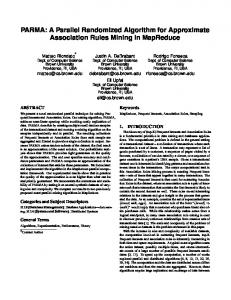
Distribution of Q for r = −5.87 and c = 3.16. P (Q = −7) = 0.02, P (Q = −6) = 0.9 and P (Q = −5) = 0.08.

Therefore, we can approximate distribution (15) by 2N -point discrete distribution as follows.  2  e−c(a+N −1) /s0 q = brc − N + 1     .. ..    . .     2  e−ca /s0 q = brc P (Q = q) = 2  −cb /s0  q = brc + 1  e    . ..  ..  .      −c(b+N −1)2 0 e /s q = brc + N where 0

s =

N −1 X

2

(37)

2

(e−c(a+i) + e−c(b+i) ).

i=0

Fig. 2 shows the distribution (15), when r = −5.87 and c = 3.16. The values of r and c are the interim results obtained by decoding an uncoded 10 × 10 system. The distribution of Q concentrates at brc = −6 and brc + 1 = −5 with probability 0.9 and 0.08 respectively. Fig. 3 compare the bit error rates associated with different N for an uncoded 10 × 10 (nT = nR = 10) system with K = 20. It is seen that the choice of N = 2 is indistinguishable from larger N . In fact, it is often adequate to choose a 3-point approximation as the probability in the central 3 points is almost one. The following lemma provides a theoretical explanation to the above argument from the viewpoint of statistical distance [35, Chap. 8]. The statistical distance measures how two probability distributions February 22, 2011

DRAFT

17 −1

10

Real−Klein−MMSE,K=20,N=1 Real−Klein−MMSE,K=20,N=2 Real−Klein−MMSE,K=20,N=5 Real−Klein−MMSE,K=20,N=10 −2

Bit Error Rate

10

−3

10

−4

10

17

17.5

18

18.5

19 19.5 E /N (dB) b

Fig. 3.

20

20.5

21

0

Bit error rate vs. average SNR per bit for a 10 × 10 uncoded system using 64-QAM.

differ from each other, and is a convenient tool to analyze randomized algorithms. An important property is that applying a deterministic or random function to two distributions does not increase the statistical distance. This implies an algorithm behaves similarly if fed two nearby distributions. More precisely, if the output satisfies a property with probability p when the algorithm uses a distribution D1 , then the property is still satisfied with probability ≥ p − ∆(D1 , D2 ) if fed D2 instead of D1 (see [35, Chap. 8]). Lemma 3: Let D (D(i) = P (Q = i)) be the non-truncated discrete Gaussian distribution, and D0 be the truncated 2N -point distribution. Then the statistical distance between D and D0 satisfies: ∆(D, D0 ) ,

1X 2 |D(i) − D0 (i)| = O(ρ−N ). 2 i∈Z

Proof: By definition of

D0 ,

∆ =

we have: 1 2

X

D(i) +

ibrc+N

DRAFT

18

where s =

P

i≥0 (e

−c(a+i)2

2

+ e−c(b+i) ) and s0 =

PN −1 i=0

2

2

(e−c(a+i) + e−c(b+i) ). The result then derives

from (35). As a consequence, the statistical distance between the distributions used by Klein’s algorithm cor2

responding to the non-truncated and truncated Gaussians is nKO(ρ−N ). Hence, the behavior of the algorithm with truncated Gaussian is almost the same. B. Complex Randomized Lattice Decoding Since the traditional lattice formulation is only directly applicable to a real-valued channel matrix, sampling decoding was given for the real-valued equivalent of the complex-valued channel matrix. This approach doubles the channel matrix dimension and may lead to higher complexity. From the complex lattice viewpoint [36], we study the complex sampling decoding. The advantage of this algorithm is that it reduces the computational complexity by incorporating complex LLL reduction [36]. Due to the orthogonality of real and imaginary part of the complex subchannel, real and imaginary part of the transmit symbols are decoded in the same step. This allows us to derive complex sampling decoding by performing randomized rounding for the real and imaginary parts of the received vector separately. In this sense, given the real part of input y, sampling decoding returns real part of z with probability 1 2 e−Ak