Programs. Thomas Ball and Sriram K. Rajamani ...... CDH+00 James Corbett, Matthew Dwyer, John Hatcli , Corina Pasareanu, Robby,. Shawn Laubach, and ...
Bebop: A Symbolic Model Checker for Boolean Programs Thomas Ball and Sriram K. Rajamani Software Productivity Tools Microsoft Research
http://www.research.microsoft.com/slam/
Abstract. We present the design, implementation and empirical evalu-
ation of Bebop|a symbolic model checker for boolean programs. Bebop represents control ow explicitly, and sets of states implicitly using BDDs. By harnessing the inherent modularity in procedural abstraction and exploiting the locality of variable scoping, Bebop is able to model check boolean programs with several thousand lines of code, hundreds of procedures, and several thousand variables in a few minutes.
1 Introduction Boolean programs are programs with the usual control- ow constructs of an imperative language such as C but in which all variables have boolean type. Boolean programs contain procedures with call-by-value parameter passing and recursion, and a restricted form of control nondeterminism. Boolean programs are an interesting subject of study for a number of reasons. First, because the amount of storage a boolean program can access at any point is nite, questions of reachability and termination (which are undecidable in general) are decidable for boolean programs.1 Second, as boolean programs contain the control- ow constructs of C, they form a natural target for investigating model checking of software. Boolean programs can be thought of as an abstract representation of C programs that explicitly captures correlations between data and control, in which boolean variables can represent arbitrary predicates over the unbounded state of a C program. As a result, boolean programs are useful for reasoning about temporal properties of software, which depend on such correlations. We have created a model checker for boolean programs called Bebop. Given a boolean program B and a statement s in B , Bebop determines if s is reachable in B (informally stated, s is reachable in B if there is some initial state such that if B starts execution from this state then s 1 Boolean programs are equivalent in power to push-down automaton, which accept
context-free languages.
decl g;
[6] [7] [8] [9] [10] [11] [12] [14]
[20] [21] [22] [24]
main() begin decl h; h := !g; A(g,h); skip; A(g,h); skip; if (g) then R: skip; else skip; fi end A(a1,a2) begin if (a1) then A(a2,a1); skip; else g := a2; fi end
bebop v1.0: (c) Microsoft Corporation. Done creating bdd variables Done building transition relations Label R reachable by following path: Line 12 Line 11 Line 10 Line 22 Line Line Line 21 Line 20 Line 9 Line 8 Line 22 Line Line Line 21 Line 20 Line 7 Line 6
24 20
24 20
State State State State State State State State State State State State State State State State State
g=1 g=1 g=1 g=1 g=1 g=1 g=1 g=1 g=1 g=1 g=1 g=1 g=1 g=1 g=1 g=1 g=1
h=0 h=0 h=0 a1=1 a1=0 a1=0 a1=1 a1=1 h=0 h=0 a1=1 a1=0 a1=0 a1=1 a1=1 h=0
a2=0 a2=1 a2=1 a2=0 a2=0
a2=0 a2=1 a2=1 a2=0 a2=0
Fig. 1. The skip statement labelled R is reachable in this boolean program, as shown by the output of the Bebop model checker.
eventually executes). If statement s is reachable, then Bebop produces a shortest trace leading to s (that possibly includes loops and crosses procedure boundaries). Example. Figure 1 presents a boolean program with two procedures (main and a recursive procedure A). In this program, there is one global variable g. Procedure main has a local variable h which is assigned the complement of g. Procedure A has two parameters. The question is: is label R reachable? The answer is yes, as shown by the output of Bebop on the right. The tool nds that R is reachable and gives a shortest trace (in reverse execution order) from R to the rst line of main (line 6). The indentation of a line indicates the depth of the call stack at that point in the trace. Furthermore, for each line in the trace, Bebop outputs the state of the variables (in scope) just before the line. The trace shows that in order to reach label R, by this trace of lines, the value of g initially must
be 1.2 Furthermore, the trace shows that the two calls that main makes to procedure A do not change the value of g. We re-emphasize that this is a shortest trace witnessing the reachability of label R. Contributions. We have adapted the interprocedural data ow analysis algorithm of Reps, Horwitz and Sagiv (RHS) [RHS95,RHS96] to decide the reachability status of a statement in a boolean program. A core idea of the RHS algorithm is to e�ciently compute \summaries" that record the input/output behavior of a procedure. Once a summary hI; Oi has been computed for a procedure pr, it is not necessary to reanalyze the body of pr if input context I arises at another call to pr. Instead, the summary for pr is consulted and the corresponding output context O is used. We use Binary Decisions Diagrams (BDDs) to symbolically represent these summaries, which are binary relationships between sets of states. In the program of Figure 1, our algorithm computes the summary s = hfg = 1; h = 0g; fg0 = 1; h0 = 0gi when procedure A is rst called (at line 7) with the state fg = 1; h = 0g. This summary will be \installed" at all calls to A (in particular, the call to A at line 9). Thus, when the state I = fg = 1; h = 0g propagates to the call at line 9, the algorithm nds that the summary s matches and will use it to \jump over" the call to A rather than descending into A to analyze it again. A key point about Bebop that distinguishes it from other model checkers is that it exploits the locality of variable scopes in a program. The time and space complexity of our algorithm is O(E � 2k ) where E is the number of edges in the interprocedural control- ow graph of the boolean program3 and k is the maximal number of variables in scope at any program point in the program. In the example program of Figure 1 there are a total of 4 variables (global g, local h, and formals a1 and a2). However, at any statement, at most three variables are in scope (in main, g and h; in A, g, a1, and a2). So, for a program with g global variables, and a maximum of l local variables in any procedure, the running time is O(E � 2g+l ). If the number of variables in scope is held constant then the running time of Bebop grows as function of the number of statements in the program (and not the total number of variables). As a result, we have been able to model check boolean programs with several thousand lines of code, and several 2 Note that g is left unconstrained in the initial state of the program. If a variable's
value is unconstrained in a particular trace then Bebop does not output it. Thus, it is impossible for g to be initially 0 and to follow the same trace. In fact, for this example, label R is not reachable if g initially is 0. 3 E is linear in the number of statements in the boolean program.
thousand variables in a few minutes (the largest example we report in Section 4 has 2401 variables). A second major idea in Bebop is to use an explicit control- ow graph representation rather than encode the control ow of a boolean program using BDDs. This implementation decision is an important one, as it allows us to optimize the model checking algorithm using well-known techniques from compiler optimization. We explain two such techniuqes |live ranges and modication/reference analysis| to reduce the number of variables in support of the BDDs that represent the reachable states at a program point. Overview. Section 2 presents the syntax and semantics of boolean programs. Section 3 describes our adaption of the RHS algorithm to use BDDs to solve the reachability problem for boolean programs. Section 4 evaluates the performance of Bebop. Section 5 reviews related work and Section 6 looks towards future work.
2 Boolean Programs 2.1 Syntax Figure 2 presents the syntax of boolean programs. We will comment on noteworthy aspects of it here. Boolean variables are either global (if they are declared outside the scope of a procedure) or local (if they are declared inside the scope of a procedure). Since there is only one type in the boolean programming language, variable declarations need not specify a type. Variables are statically scoped, as in C. A variable identi er is either a C-style identifer or an arbitrary string between the characters \f\ and \g". The latter form is useful for creating boolean variables with names denoting predicates in another language (such as f*p==*qg). There are two constants in the language: 0 (false) and 1 (true). Expressions are built in the usual way from these constants, variables and the standard logical connectives. The statement sub-language (stmt) is very similar to that of C, with a few exceptions. Statements may be labelled, as in C. A parallel assignment statement allows the simultaneous assignment of a set of values to a set of variables. Procedure calls use call-by-value parameter passing.4 There 4 Boolean programs support return values from procedures, but to simplify the techni-
cal presentation we have omitted their description here. A return value of a procedure can be modelled with a single global variable, where the global variable is assigned immediately preceding a return and copied immediately after the return into the local state of the calling procedure.
Syntax
Description
prog ::= decl � proc � decl ::= decl id + ; id ::= [a-zA-Z ] [a-zA-Z0-9 ] �
j
f string g
proc ::= id ( id � ) begin decl � sseq end sseq ::= lstmt + lstmt ::= stmt j id : stmt stmt ::= skip ; j print ( expr + ) ; j goto id ;
return ; id + := expr + ; if ( decider ) then sseq else sseq while ( decider ) do sseq od assert ( decider ); id ( expr � ) ; decider ::= ? j expr j j j j j j
A program is a list of global variable declarations followed by a list of procedure de nitions Declaration of variables An identi er can be a regular C-style identi er or a string of characters between 'f' and 'g' Procedure de nition Sequence of statements Labelled statement
Parallel assignment Conditional statement Iteration statement Assert statement Procedure call Non-deterministic choice
expr ::= expr binop expr j ! expr Negation j ( expr ) j id j const binop ::= 'j' j '&' j '^' j '=' j '!=' j ')' Logical connectives const ::= 0 j 1 False/True
Fig. 2. The syntax of boolean programs.
are three statements that can a�ect the control ow of a program: if , while and assert. Note that the predicate of these three statements is a decider, which can be used to model non-determinism. A decider is either a boolean expression which evaluates (deterministically) to 0 or 1, or \?", which evaluates to 0 or 1 non-deterministically.
2.2 Statements, Variables and Scope The term statement denotes an instance that can be derived from the nonterminal stmt (see Figure 2). Let B be a boolean program with n statements and p procedures. We assign a unique index to each statement
in B in the range 1 : : : n and a unique index to each procedure in B in the range n + 1 : : : n + p. Let si denote the statement with index i. To simplify presentation of the semantics, we assume that variable names and statement labels are globally unique in B . Let V (B ) be the set of all variables in B . Let Globals (B ) be the set of global variables of B . Let FormalsB (i) be the set of formal parameters of the procedure that contains si. Let LocalsB (i) be the set of local variables and formal parameters of the procedure that contains si . For all i, 1 � i � n, FormalsB (i) � LocalsB (i). Let InScopeB (i) denote the set of all variables of B whose scope includes si . For all i, 1 � i � n, InScopeB (i) = LocalsB (i) [ Globals (B ).
2.3 The Control- ow Graph
This section de nes the control- ow graph of a boolean program. Since boolean programs contain arbitrary intra-procedural control ow (via the goto), it is useful to present the semantics of boolean programs in terms of their control- ow graph rather than their syntax. To make the presentation of the control- ow graph simpler, we make the minor syntactic restriction that every call c to a procedure pr in a boolean program is immediately followed by a skip statement skipc . The control- ow graph of a boolean program B is a directed graph GB = (VB ; SuccB ) with set of vertices VB = f1; 2; : : : ; n + p + 1g and successor function SuccB : VB ! 2VB . The set VB contains one vertex for each statement in B (vertices 1 : : : n) and one vertex Exit pr for every procedure pr in B (vertices n + 1 : : : n + p). In addition, VB contains a vertex Err = n + p + 1 which is used to model the failure of an assert statement. For any procedure pr in B , let FirstB (pr) be the index of the rst statement in pr. For any vertex v 2 VB , fErr g, let ProcOfB (v) be the index of the procedure containing v. The successor function SuccB is de ned in terms of the function NextB : f1; 2; : : : ; ng ! f1; 2; : : : ; n + pg which maps statement indices to their lexical successor if one exists, or to the exit node of the containing procedure otherwise. NextB (i) has a recursive de nition based on the syntax tree of B (see Figure 2). In this tree, each statement has an sseq node as its parent. The sequence of statements derived from the sseq parent of statement si is called the containing sequence of si . If si is not the last statement in its containing sequence then NextB (i) is the index of the statement immediately following si in this sequence. Otherwise, let a be the closest ancestor of si in the syntax tree such that (1) a is a stmt node, and (2) a is not the last statement in a's containing sequence. If such a
node a exists, then NextB (i) is the index of the statement immediately following a in its containing sequence. Otherwise, NextB (si ) = Exit pr , where pr = ProcOfB (i). If sj is a procedure call, we de ne ReturnPtB (j ) = NextB (j ) (which is guaranteed to be a skip statement because of the syntactic restriction we previously placed on boolean programs). We now de ne SuccB using NextB and ReturnPtB . For 1 � i � n, the value of SuccB (i) depends on the statement si , as follows: { If si is \goto L" then SuccB (i) = fj g, where sj is the statement labelled L. { If si is a parallel assignment, skip or print statement then SuccB (i) = fNextB (i)g. { If si is a return statement then SuccB (i) = fExit prg, where pr = ProcOfB (i). { If si is an if statement then SuccB (v) = fTsuccB (i); FsuccB (i)g, where TsuccB (i) is the index of the rst statement in the then branch of the if and FsuccB (i) is the index of the rst statement in the else branch of the if . { If si is a while statement then SuccB (i) = fTsuccB (i); FsuccB (i)g, where TsuccB (i) is the rst statement in the body of the while loop and FsuccB (i) = NextB (i). { If si is an assert statement then SuccB (i) = fTsuccB (i); FsuccB (i)g, where TsuccB (i) = NextB (i) and FsuccB (i) = n + p + 1 (the Err vertex). { If si is a procedure call to procedure pr then SuccB (i) = FirstB (pr). We now de ne SuccB (i) for n +1 � i � n + p (that is, for the Exit vertices associated with the p procedures of B ). Given exit vertex Exit pr for some procedure pr, we have SuccB (Exit pr ) = fReturnPtB (j ) j statement sj is a call to pr g Finally, SuccB (Err ) = fg. That is, the vertex Err has no successors. The control- ow graph of a boolean program can be constructed in time and space linear n + p, the number of statements and procedures in the program.
2.4 A Transition System for Boolean Programs For a set V � V (B ), a valuation to V is a function that associates
every boolean variable in V with a boolean value. can be extended to
expressions over V (see expr in Figure 2) in the usual way. For example, if V = fx; yg, and = f(x; 1); (y; 0)g then (xjy) = 1. For any function f : D ! R, d 2 D, r 2 R, f [d=r] : D ! R is de ned as f [d=r](d0 ) = r if d = d0 , and f (d0 ) otherwise. For example, if V = fx; yg, and = f(x; 1); (y; 0)g then [x=0] = f(x; 0); (y; 0)g: A state � of B is a pair hi; i, where i 2 VB and is a valuation to the variables in InScopeB (i). States (B ) is the set of all states of B . Intuitively, a state contains the program counter (i) and values to all the variables visible at that point ( ). Note that our de nition of state is di�erent from the conventional notion of a program state, which includes a call stack. The projection operator , maps a state to its vertex: , (hi; i) = i. We can extend , to operate on sequences of states in the usual way. We de ne a set � (B ) of terminals:
� (B ) = f�g [ f hcall; i; �i; hret; i; �i j 9j 2 VB ; sj is a procedure call; i = ReturnPtB (j ); and � is a valuation to LocalsB (j )g It is clear that � (B ) is nite since all variables in B are boolean variables. Terminals are either �, which is a place holder, or triples that are introduced whenever there is a procedure call in B . The rst component of the triple is either call or ret, corresponding to the actions of a call to and return from that procedure, the second is the return point of the call, and the third component keeps track of values of local variables of the calling procedure at the time of the call. We use �1 !�B �2 , to denote that B can� make an �-labeled transition from state �1 to state �2 . Formally, �1 !B �2 holds if �1 = hi1 ; 1 i 2 States (B ), �2 = hi2 ; 2 i 2 States (B ), and � 2 � (B ), where the conditions on �1 , �2 and � for each statement construct are shown in Table 1. We explain the table below:
{ The transitions for skip, print, goto and return are the same. All these statements have exactly one control- ow successor. For vertices v such that SuccB (v) = fwg, we de ne sSuccB (v) = w. Each statement passes control to its single successor sSuccB (i1 ) and does not change the state of the program. { The transition for parallel assignment again passes control to the sole successor of the statement and the state changes in the expected manner. { The transitions for if , while and assert statements are identical. If the value of the decider d associated with the statement is ? then
i1 skip print goto return x1 ; : : : ; xk := e1 ; : : : ; ek
�
i2
2
�=�
i2 = sSuccB (i1 )
2 = 1
1 [x1 = 1 (e1 ))] i2 = sSuccB (i1 ) �2� �=[x k =
1 (ek )] if d = ? i2 2 SuccB (i1 ) if (d) if
1 (d) = 1 while(d) �=�
2 = 1 i = TsuccB (i1 ) 2 assert(d) if 1 (d) = 0 i2 = FsuccB (i1 )
2 (xi ) = 1 (ei ); � = h call ; ReturnPt ( i ) ; � i , B (i2 ) B 1 pr(e1 ; : : : ; ek ) �(x) = 1 (x); 8 x 2 LocalsB (i1 ) i2 = FirstB (pr) 82 x(gi )2=Formals
1 (g); 8 g 2 Globals (B )
2 (g) = 1 (g); (B ) Exit pr � = hret; i2 ; �i i2 2 SuccB (i1 ) 82 g(x2) =Globals �(x); 8 x 2 LocalsB (i2 ) � Table 1. Conditions on the state transitions hi1 ; 1 i!B hi2 ; 2 i, for each vertex type of i1 . See the text for a full explanation.
�=�
the successor is chosen non-deterministically from the set SuccB (i1 ). Otherwise, d is a boolean expression and is evaluated in the current state to determine the successor. { The transition for a call statement si1 contains the � label hcall; ReturnPtB (i1 ); �i where � records the values of the local variables at i1 from the state
1 . The next state, 2 gives new values to the formal parameters of the called procedure based on the values of the corresponding actual arguments in state 1 . Furthermore, 2 is constrained to be the same as 1 on the global variables. { Finally, the transition for an exit vertex i1 = Exit pr has � = hret; i2 ; �i, where i2 must be a successor of i1 . The output state 2 is constrained as follows: 2 must agree with 1 on all global variables; 2 must agree with � on the local variables in scope at i2 .
2.5 Trace Semantics
We now are in a position to give a trace semantics to boolean programs based on a context-free grammar G (B ) over the alphabet � (B ) that spec-
1. S ! MS 4. 8hcall; i; �i; hret; i; �i 2 � (B ) : 2. 8hcall; i; �i 2 � (B ) : M ! hcall; i; �i M hret; i; �i S ! hcall; i; �i S 5. M ! MM 3. S ! � 6. M ! � 7. M ! � Table 2. The production rules Rules (B ) for grammar G (B ).
i es the legal sequences of calls and returns that a boolean program B may make. A context-free grammar G is a 4-tuple hN; T; R; S i, where N is a set of nonterminals, T is a set of terminals, R is a set of production rules and S 2 N is a start symbol. For each program B , we de ne a grammar G (B ) = hfS; M g; � (B ); Rules (B ); S i, where Rules (B ) is de ned by the productions of Table 2. If we view the terminals hcall; i; �i and hret; i; �i from � (B ) as matching left and right parentheses, the language L(G (B )) is the set of all strings over � (B ) that are sequences of partially-balanced parentheses. That is, every right parenthesis hret; i; �i is balanced by a preceding hcall; i; �i but the converse need not hold. The � component insures that the values of local variables at the time of a return are the same as they were at the time of the corresponding call (this must be the case because boolean programs have a call-by-value semantics). The nonterminal M generates all sequences of balanced calls and returns, and S generates all sequences of partially balanced calls and returns. This allows us to reason about non-terminating or abortive executions. Note again that the number of productions is nite because B contains only boolean variables. We assume that B contains a distinguished procedure named main, which is the initial procedure that executes. A state � = hi; i is initial if i = FirstB (main) (all variables can take on arbitrary initial values). A �m nite sequence � = �0 !�1B �1 !�2B � � � �m,1 ! B �m is a trajectory of B if (1) �i for all 0 � i < m, �i !B �i+1 , and (2) �1 : : : �m 2 L(G (B )). A trajectory � is called an initialized trajectory if �0 is an initial state of B . If � is an initialized trajectory, then its projection to vertices , (�0 ); , (�1 ); : : : ; , (�n ) is called a trace of B . The semantics of a boolean program is its set of traces. A state � of B is reachable if there exists an initialized trajectory of B that ends in �. An vertex v 2 VB is reachable if there exists a trace of B that ends in vertex v.
3 Boolean Programs Reachability via Interprocedural Data ow Analysis and BDDs In this section, we present an interprocedural data ow analysis that, given a boolean program B and its control- ow graph GB = (VB ; SuccB ), determines the reachability status of every vertex in VB . We describe and present the algorithm, show how it can be extended to report short trajectories (when a vertex is found to be reachable), and describe several optimizations that we plan to make to the algorithm.
3.1 The RHS Algorithm, Generalized As discussed in the Introduction, we have generalized the interprocedural data ow algorithm of Reps-Horwitz-Sagiv (RHS) [RHS95,RHS96]. The main idea of this algorithm is to compute \path edges" that represent the reachability status of a vertex in a control- ow graph and to compute \summary edges" that record the input/output behavior of a procedure. We (re)de ne path and summary edges as follows: Path edges. Let v be a vertex in VB and let e = FirstB (ProcOfB (v)). A path edge incident into a vertex v, is a pair of valuations h e ; v i,5 such that(1) there is a initialized trajectory � 1 = hFirstB (main); i : : : he; e i, and (2) there is a trajectory � 2 = he; e i : : : hv; v i that does not contain the exit vertex Exit ProcOfB (v) (exclusive of v itself). For each vertex v, PathEdges (v) is the set of all path edges incident into v. A summary edge is a special kind of path edges that records the behavior of a procedure. Summary edges. Let c be a vertex in VB representing a procedure call with corresponding statement sc = pr(e1 ; e2 ; :::ek ). A summary edge associated with c is a pair of valuations h 1 ; 2 i, such that all the local variables in LocalsB (c) are equal in 1 and 2 , and the global variables change according to some path edge from the entry to the exit of the callee. Suppose P is the set of path edges at Exit pr . We de ne Lift c (P; pr) as the set of summary edges obtained by \lifting" the set of path edges P to the call c, while respecting the semantics of the call and return
e and v are de ned with respect to the set of variables InScopeB (e) = InScopeB (v).
5 The valuations
V =
transitions from Table 1. Formally Lift c (P; pr) = fh 1 ; 2 i j9h i ; o i 2 P; and 8x 2 LocalsB (c) : 1 (x) = 2 (x); and 8x 2 Globals (B ) : ( 1 (x) = i (x)) ^ ( 2 (x) = o(x)); and 8 formals yj of pr and actuals ej : 1 (ej ) = i (yj )g
For each vertex v in CallB , SummaryEdges (v) is the set of summary edges associated with v. As the algorithm proceeds, SummaryEdges (v) is incrementally computed for each call site. Summary edges are used to avoid revisiting portions of the state space that have already been explored, and enable analysis of programs with procedures and recursion. Let CallB be the set of vertices in VB that represent call statements. Let ExitB be the set of exit vertices in VB . Let CondB be the set of vertices in VB that represent the conditional statements if , while and assert. Transfer Functions. With each vertex v such that sv 62 CondB [ ExitB , we associate a transfer function Transfer v . With each vertex v 2 CondB , we associate two transfer functions Transfer v;true and Transfer v;false . The de nition of these functions is given in Table 3. Given two sets of pairs of valuations, S and T , Join (S; T ) is the image of set S with respect to the transfer function T . Formally Join (S; T ) = fh 1 ; 2 i j 9 j :h 1 ; j i 2 S ^ h j ; 2 i 2 T g. During the processing of calls, in addition to applying the transfer function, the algorithm uses the function SelfLoop which takes a set of path edges, and makes self-loops with the targets of the edges. Formally, SelfLoop (S ) = fh 2 ; 2 i j 9h 1 ; 2 i 2 S g. Our generalization of the RHS algorithm is shown in Figure 3. The algorithm uses a worklist, and computes path edges and summary edges in a directed, demand-driven manner, starting with the entry vertex of main (the only vertex initially known to be reachable). In the algorithm, path edges are used to compute summary edges, and vice versa. In our implementation, we use BDDs to represent transfer functions, path edges, and summary edges. As is usual with BDDs, a boolean expression e denotes the set of states e = f j (e) = 1g. A set of pairs of states can easily be represented with a single BDD using primed versions of the variables in V (B ) to represent the variables in the second state. Since transfer functions, path edges, and summary edges are sets of pairs of states, we can represent and manipulate them using BDDs. Upon termination of the algorithm, the set of path edges for a vertex v is empty i� v is not reachable. If v is reachable, we can generate a shortest trajectory to v, as described in the next section.
global
PathEdges ,SummaryEdges ,WorkList
procedure Propagate(v,p) begin if p 6� PathEdges (v) then PathEdges (v) := PathEdges (v) [ p Insert v into WorkList end procedure Reachable(GB ) begin for all v 2 VB do PathEdges (v) := fg for all v 2 CallB do SummaryEdges (v) := fg PathEdges (FirstB (main)) := fh ; i j is any valuation to globals and local variables of maing WorkList := fFirstB (main)g while WorkList =6 ; do remove vertex v from WorkList switch (v) case v 2 CallB : Propagate(sSuccB (v),SelfLoop (Join (PathEdges (v); Transfer v ))) Propagate(ReturnPtB (v),Join (PathEdges (v); SummaryEdges (v))) case v 2 ExitB : for each w 2 SuccB (v) do let c 2 CallB such that w = ReturnPtB (c) and s = Lift c (PathEdges (v); ProcOfB (v)) in if s 6� SummaryEdges (c) then SummaryEdges (c) := SummaryEdges (c) [ s Propagate(w,Join (PathEdges (c); SummaryEdges (c))); ni case v 2 CondB : Propagate(TsuccB (v); Join (PathEdges (v); Transfer v;true )) Propagate(FsuccB (v); Join (PathEdges (v); Transfer v;false )) case v 2 VB , CallB , ExitB , CondB : let p = Join (PathEdges (v); Transfer v ) in for each w 2 SuccB (v) do Propagate(w,p) ni end Fig. 3. The model checking algorithm.
v Transfer v skip print �h 1 ; 2 i:( 2 = 1 ) goto return x1 ; : : : ; xk := �h 1 ; 2 i:( 2 = 1 [x1 = 1 (e1 ))] � � � [xk = 1 (ek )]) e1 ; : : : ; ek if (d) v;true = �h 1 ; 2 i:(( 1 (d) = 1) ^ ( 2 = 1 )) while(d) Transfer Transfer v;false = �h 1 ; 2 i:(( 1 (d) = 0) ^ ( 2 = 1 )) assert(d) h 1 ; 2 i:( 2 = 1 [x1 = 1 (e1 )] : : : [xk = 1 (ek )]), pr(e1 ; : : : ; ek ) �where x1 ; : : : ; xk are the formal parameters of pr. Table 3. Transfer functions associated with vertices. These are derived directly from the transition rules given in Table 1
3.2 Generating a Shortest Trajectory to a Reachable Vertex
We now describe a simple extension to the algorithm of Figure 3 to keep track of the length of the shortest hierarchical trajectory needed to reach each state, so that if vertex v is reachable, we can produce a shortest initialized hierarchical trajectory that ends in v. A hierarchical trajectory can \jump over" procedure calls using�summ� mary edges. Formally, a nite sequence � = �0 !�1B �1 !�2B � � � �m,1�! B m i is a hierarchical trajectory of B if for all 0 � i < m, (1) either �i !B �i+1 , or �i = hvi ; i i, �i+1 = hvi+1 ; i+1 i, �i = �, vi 2 CallB and h i ; i+1 i 2 SummaryEdges (vi ), and (2) �1 : : : �m 2 L(G (B )). Let v be a vertex and let e = FirstB (ProcOfB (v)). For a path edge h e; v i 2 PathEdges (v) let W (h e ; v i) be the set of all hierarchical trajectories that start from main, enter into the procedure ProcOfB (v) with valuation e and then reach v with valuation v without exiting ProcOfB (v). Note that a hierarchical trajectory in W (h e ; v i) is comprised of intraprocedural edges, summary edges, and edges that represent calling a procedure (but not the edges representing a return from a procedure). Instead of keeping all the path edges incident on v as a single set PathEdges (v), we partition it into a set of sets fPathEdges r1 (v); PathEdges r2 (v); : : : ; PathEdges rk (v)g where a path edge h e ; v i is in PathEdges rj (v) i� the shortest hierarchical trajectory in W ((h e ; v i) has length rj . The set fr1 ; r2 ; : : : ; rk g is called the set of rings associated with v. We use rings to generate shortest hierarchical trajectories. If vertex v is reachable, we nd the smallest ring r such that PathEdges r (v) exists.
Then we pick an arbitrary path edge h e ; v i from PathEdges r (v), and do the following depending on the type of vertex v: { If v 6= FirstB (ProcOfB (v)) then we have two subcases: � If sv is not a skip immediately following a call, then we look for a predecessor u of v such that there exists path edge h e ; u i in PathEdges r,1 (u), and Join (fh e ; u ig; Transfer u ) contains h e ; v i. � If sv is a skip immediately following a call (say at vertex u), then we look for a path edge h e ; u i in PathEdges r,1 (u) such that Join (fh e ; u ig; SummaryEdges (u)) contains h e ; v i. { If v = FirstB (ProcOfB (v)), then it should be the case that e = v, and v = e . We nd a caller u of ProcOfB (v), and suitably \lift"
v to a suitable path edge in PathEdges (u). Formally, we nd a vertex u 2 CallB such that su is a call to procedure ProcOfB (v), and there exists path edge h e0 ; u i in PathEdges r,1 (u) satisfying Transfer u (h u ; v i). Repeating this process with the vertex u and the path edge found in PathEdges r,1 (u), we are guaranteed to reach the entry of main in r steps. We may traverse over summary edges in the process. However, we can expand the summary edges on demand, to produce a hierarchical error trajectory, as shown in the Bebop output in Figure 1.
3.3 Optimizations
The basic algorithm described above has been implemented in the Bebop model checker. In this section, we describe a few optimizations based on ideas from compiler optimization [ASU86] that should substantially reduce the size of the BDDs needed to perform the analysis. Live Ranges. If for some path starting at a vertex v in the control- ow graph GB , the variable x is used before being de ned, then variable x is said to be live at v. Otherwise, x is said to be dead at v, for its value at v will not ow to any other variable. If variable x is not live at vertex v then we need not record the value of x in the BDD for PathEdges (v). Consider the following boolean program void main() begin decl a,b,c,d,e,f; L1: a := b|c; // {b,c,e} live at L1 L2: d := a|e; // {a,e} live at L2 L3: e := d|e; // {d,e} live at L3 L4: f := d; // {d} live at L4 end
This program declares and refers to six variables, but at most three variables are live at any time. For example, at the statement labelled L1 only the values of the variables b, c, and e can ow to the statements after L1. As a result, the BDD for the rst statement need not track the values of the variables a or d. MOD/REF sets. A traditional \MOD/REF" (modi cation/reference) analysis of a program determines the variables that are modi ed and/or referenced by each procedure pr (and the procedures it calls transitively). Let pr be a procedure in B such that pr nor any of the procedures it calls (transitively) modi es or references global variable g. Although g may be in scope in pr, and may in fact be live within pr, the procedure pr cannot change the value of g. As a result, all that is needed is to record that g remains unchanged, for any summary of pr.
4 Evaluation In this section, we present an evaluation of Bebop on a series of synthetic programs derived from the template T shown in Figure 4. The template allows us to generate boolean programs T (N ) for N > 0. The boolean program T (N ) has one global variable g and N + 1 procedures |a procedure main, and N procedures of the form level for 0 < i � N . For 0 < j < N , the two instances of in the body of procedure level are replaced by a call to procedure level. The two instances of in the body of procedure level are replaced by skip. As a result, a boolean program T (N ) has N + 1 procedures, where main calls level1 twice, level1 calls level2 twice, etc. At the beginning of each level procedure, a choice is made depending on the value of g. If g is 1 then a loop is executed that implements a three bit counter over the local variables a, b, and c. If g is 0 then two calls in succession are made to the next level procedure. In the last level procedure, if g is 0 then two skip statements are executed. At the end of each level procedure, the global variable g is negated. Every program T (N ) generated from this template has four variables visible at any program point, regardless of N . Note that g is not initialized, so Bebop will explore all possible values for g. We ran Bebop to compute the reachable states for boolean programs T (N ) in 0 < N � 800, and measured the running time, and peak memory used. Figure 4(a) shows how the running time of Bebop (in seconds) varies
void level() begin decl a,b,c; if(g) then a,b,c := 0,0,0; while(!a|!b|!c) do if (!a) then a := 1; elsif (!b) then a,b := 0,1; elsif (!c) then a,b,c := 0,0,1; fi od else ; ; fi g := !g; end
Running time for T(N)
Running time for T(N) (seconds)
300 250 200 CU
150
CMU
100 50 0 0
200
400
600
800
1000
N
(a) Peak Live BDD Nodes 250000 200000 Peak Space for T(N)
decl g; void main() begin level1(); level1(); if(!g) then reach: skip; else skip; fi end
150000 100000 50000 0 0
200
400
600
800
1000
N
(b)
Fig. 4. Boolean program template T for performance test and performance results.
with N . Figure 4(b) shows how the peak memory usage of Bebop varies with N . The two curves in Figure 4(a) represent two di�erent BDD packages: CU is the CUDD package from Colorado University [Som98] and CMU is the BDD package from Carnegie Mellon University [Lon93]. We note that the program T (800) has 2401 variables. Model checking of this program takes a minute and a half with the CMU package and four and a half minutes with the CUDD package. Both times are quite reasonable considering the large number of variables (relative to traditional uses of BDDs). The space measurements in Figure 4(b) are taken from the CUDD package, which provides more detailed statistics of BDD space usage.
We expected the peak memory usage to increase linearly with N . The sublinear behavior observed in Figure 4(b) is due to more frequent garbage collection at larger N . We expected the running time also to increase linearly with N . However, Figure 4(a) shows that the running time increases quadratically with N . The quadratic increase in running time was unexpected, since the time complexity of model checking program T (N ) is O(N ) (there are 4 variables in the scope of any program point). By pro ling the runs and reading the code in the BDD packages, we found that the quadratic behavior arises due to an ine�ciency in the implementation of bdd substitute in the BDD package. Bebop calls bdd substitute in its \inner loop", since variable renaming is an essential component of its forward image computation. While model checking T (N ), the BDD manager has O(N ) variables, but we are interested in substituting O(n) variables, for a small n, using bdd substitute. Regardless of n, we found that bdd substitute still consumes O(N ) time. Both the CUDD and CMU packages had this ine�ciency. If this ine�ciency is xed in bdd substitute, we believe that the running time of Bebop for T (N ) will vary linearly with N .
5 Related Work Model checking for nite state machines is a well studied problem, and several model checkers |SMV [McM93], Mur� [Dil96], SPIN [HP96], COSPAN [HHK96], VIS [BHSV+ 96] and MOCHA [AHM+ 98]| have been developed. Boolean programs implicitly have an unbounded stack, which makes them identical in expressive power to pushdown automata. The model checking problem for pushdown automata has been studied before [SB92] [BEM97] [FWW97]. Model checkers for push down automata have also been written before [EHRS00]. However, unlike boolean programs, these approaches abstract away data, and concentrate only on control. As a result spurious paths can arise in these models due to information loss about data correlations. The connections between model checking, data ow analysis and abstract interpretation have been explored before [Sch98] [CC00]. The RHS algorithm [RHS95,RHS96] builds on earlier work in interprocedural data ow analysis from [KS92] and [SP81]. We have shown how this algorithm can be generalized to work as a model checking procedure for boolean programs. Also, our choice of hybrid representation of the state space in Bebop|an explicit representation of control ow and an implicit BDD-based representation of path edges and summary edges| is novel.
Exploiting design modularity in model checking has been recognized as a key to scalability of model checking [AH96] [AG00] [McM97] [HQR98]. The idea of harnessing the inherent modularity in procedural abstraction, and exploiting locality of variable scoping for e�ciency in model checking software is new, though known in the area of data ow analysis [RHS96]. Existing model checkers neither support nor exploit procedural abstraction. As a result, existing approaches to extract models from software are forced to inline procedure de nitions at their points of invocation [CDH+ 00], which could lead to explosion in both the size of the model and the number of variables.
6 Future Work is part of a larger e�ort called SLAM6 , in progress at Microsoft Research, to extract abstract models from code and check temporal properties of software. We are currently implementing a methodology that uses boolean programs, and an iterative re nement process using path simulation to model check critical portions of operating system code [BR00]. Bebop
References [AG00]
A. Alur and R. Grosu. Modular re nement of hierarchic reactive modules. In POPL 00: Principles of Programming Languages. ACM Press, 2000. [AH96] R. Alur and T.A. Henzinger. Reactive modules. In LICS 96: Logic in Computer Science, pages 207{218. IEEE Computer Society Press, 1996. [AHM+ 98] R. Alur, T.A. Henzinger, F.Y.C. Mang, S. Qadeer, S.K. Rajamani, and S. Tasiran. Mocha : Modularity in model checking. In CAV 98: Computer Aided Veri cation, LNCS 1427, pages 521{525. Springer-Verlag, 1998. [ASU86] A. Aho, R. Sethi, and J. Ullman. Compilers: Principles, Techniques and Tools. Addison-Wesley, Reading, MA, 1986. [BEM97] A. Bouajjani, J. Esparza, and O. Maler. Reachability analysis of pushdown automata: Application to model-checking. In CONCUR 97: Concurrency Theory, LNCS 1243, pages 135{150. Springer-Verlag, 1997. [BHSV+96] R.K. Brayton, G.D. Hachtel, A. Sangiovanni-Vincentelli, F. Somenzi, A. Aziz, S.-T. Cheng, S. Edwards, S. Khatri, Y. Kukimoto, A. Pardo, S. Qadeer, R.K. Ranjan, S. Sarwary, T.R. Shiple, G. Swamy, and T. Villa. VIS: A System for Veri cation and Synthesis. In CAV 96: Computer Aided Veri cation, LNCS 1102, pages 428{432. Springer-Verlag, 1996. [BR00] T. Ball and S. K. Rajamani. Boolean programs: A model and process for software analysis. Technical Report MSR-TR-2000-14, Microsoft Research, February 2000. [Bry86] R.E. Bryant. Graph-based algorithms for boolean function manipulation. IEEE Transactions on Computers, C-35(8):677{691, 1986. 6
http://www.research.microsoft.com/slam/
[CC00]
P. Cousot and R. Cousot. Temporal abstract interpretation. In POPL 00: Principles of Programming Languages. ACM Press, 2000. [CDH+ 00] James Corbett, Matthew Dwyer, John Hatcli�, Corina Pasareanu, Robby, Shawn Laubach, and Hongjun Zheng. Bandera : Extracting nite-state models from java source code. In ICSE 2000: International Conference on Software Engineering, 2000. [Dil96] D. L. Dill. The Mur� Veri cation System. In CAV 96: Computer Aided Veri cation, LNCS 1102, pages 390{393. Springer-Verlag, 1996. [EHRS00] J. Esparza, D. Hansel, P. Rossmanith, and S. Schwoon. E�cient algorithms for model checking pushdown systems. Technical Report TUMI0002, SFB-Bericht 342/1/00 A, Technische Universitat Munchen, Institut fur Informatik, February 2000. [FWW97] A. Finkel, B. Willems, and P. Wolper. A direct symbolic approach to model checking pushdown systems. In INFINITY' 97: Veri cation of In nitestate Systems, July 1997. [HHK96] R.H. Hardin, Z. Har'El, and R.P. Kurshan. COSPAN. In CAV 96: Computer Aided Veri cation, LNCS 1102, pages 423{427. Springer-Verlag, 1996. [HP96] G.J. Holzmann and D.A. Peled. The State of SPIN. In CAV 96: Computer Aided Veri cation, LNCS 1102, pages 385{389. Springer-Verlag, 1996. [HQR98] T.A. Henzinger, S. Qadeer, and S.K. Rajamani. You assume, we guarantee: methodology and case studies. In CAV 98: Computer Aided Veri cation, LNCS 1427, pages 440{451. Springer-Verlag, 1998. [KS92] J. Knoop and B. Ste�en. The interprocedural coincidence theorem. In CC 92: Compiler Construction, LNCS 641, pages 125{140, Springer-Verlag, 1992. [Lon93] D. Long. Cmu bdd package. http://emc.cmu.edu/pub, Carnegie Melon University, 1993. [McM93] K.L. McMillan. Symbolic Model Checking: An Approach to the StateExplosion Problem. Kluwer Academic Publishers, 1993. [McM97] K.L. McMillan. A compositional rule for hardware design re nement. In CAV 97: Computer-Aided Veri cation, LNCS 1254, pages 24{35. SpringerVerlag, 1997. [RHS95] T. Reps, S. Horwitz, and M. Sagiv. Precise interprocedural data ow analysis via graph reachability. In POPL 95: Principles of Programming Languages, pages 49{61. ACM Press, 1995. [RHS96] T. Reps, S. Horwitz, and M. Sagiv. Precise interprocedural data ow analysis with applications to constant propagation. Theoretical Computer Science, 167:131{170, 1996. [SB92] B. Ste�en and O. Burkart. Model checking for context-free processes. In CONCUR 92: Concurrency Theory, LNCS 630, pages 123{137. SpringerVerlag, 1992. [Sch98] D.A. Schmidt. Data ow analysis is model checking of abstract interpretation. In POPL 98: Principles of Programming Languages, pages 38{48. ACM Press, 1998. [Som98] F. Somenzi. Colorado university decision diagram package. ftp://vlsi.colorado.edu/pub, University of Colorado, Boulder, 1998. [SP81] M. Sharir and A. Pnueli. Two approaches to interprocedural data dalow analysis. In Program Flow Analysis: Theory and Applications, pages 189{ 233. Prentice-Hall, 1981.