Parallelizing the Spin Model Checker Gerard J. Holzmann Laboratory for Reliable Software, Jet Propulsion Laboratory, California Institute of Technology, Pasadena, CA 91109, USA
[email protected]
Abstract. We describe an extension of the Spin model checker that allows us to take advantage of the increasing number of cpu-cores available on standard desktop systems. Our main target is to speed up the verification process for safety properties, the mode used most frequently, but we also describe a small modification of the parallel search algorithm, called the piggyback algorithm, that is remarkably effective in catching violations for an interesting class of liveness properties at little cost. Keywords: parallelism, concurrency, multi-core, model checking, Spin, breadth-first search, safety, liveness, bounded search, software verification
1
Introduction
We build on the infra-structure provided by the model checker Spin [5]. Although the model checker targets the analysis of multi-threaded software applications, until recently the tool itself performed its analyses single-threaded, using just a single cpu. In 2005 a modification was introduced that allowed for the execution of the depth-first search analysis on multiple cpu-cores [6]. This extension was chosen because it can support both safety and liveness properties, yet for liveness properties the depth-first algorithm could only take advantage of parallel execution on no more than two cpu-cores. Parallelization of breadth-first search is often considered simpler, and could lead to greater gains, so it is attractive to support also this option, even if it means restricting it to the verification of safety properties alone. The parallel version of the breadth-first search described in this paper requires virtually no tuning or user adjustments and succeeds in providing an impressive performance improvement in the model checking process. We also show that a simple extension of this algorithm suffices to support also the verification of an interesting class of liveness properties without measurable overhead. The remainder of this paper is organized as follows. In Section 2 we describe the basic breadth-first search algorithm that is used in Spin. In Section 3 we describe the parallelization of this algorithm, where we focus on the key issues of load balancing, lock avoidance, and partial order reduction. In Section 4 we discuss an extension that supports checks for liveness properties with a bounded cycle search option.
2
Parallelizing the Spin Model Checker
Section 5 presents documents the performance of the new algorithm when applied to a range of verification problems. Section 6, concludes the paper and summarizes the key results.
2
Breadth-First Search
Figure 1 gives the basic sequential algorithm for performing a breadth-first in a reachability graph, as used in the Spin model checker. The algorithm uses three sets of states: S, Q[0], and Q[1]. Set S is the set of visited states, which is initially empty. Every new state that is encountered during the search is entered into this set, to avoid duplicate work when the state is revisited later. Set S is typically implemented as a hashtable. 1 2 3 4 5 6 7 8 9 10 11 12 13 14 15 16 17 18 19 20 21 22 23
global global global global safety
t = 0 // S = {} // Q[0] = {} // Q[1] = {} // property f
toggle bit 0..1 statespace set successor set successor set
add s0 to Q[0] and to S
// initial state
Search() do { for each s in Q[t] { delete s from Q[t] for each successor s’ of s { if s’ not in S { add s’ to S if s’ violates f { report safety violation } else { add s’ to Q[1-t] } } } } t = 1 - t } while (Q[t] is non-empty) }
Fig. 1. Sequential breadth-first search.
The breadth-first search proceeds by repeatedly generating the set of successor states (the ’next’ generation) for a given set of states (the ’current’ generation). These two sets are stored in successor sets Q[0] and Q[1]. As soon as all states in the ’current’ generation of states have been processed, the roles of Q[0] and Q[1] switch, and what was the ’next’ generation of states becomes the new ’current’ generation, and the now empty former ’current’ generation becomes
Parallelizing the Spin Model Checker
3
the temporary holding place for the new ’next’ generation of states. In Figure 1 this switch happens by toggling the value of t on line 21. Every new state that is processed (i.e., each successor to one of the states from the ’current’ generation of states) is first checked for its presence in S (line 14). If new, one or more safety properties can be checked for this state (line 16), and violations reported (line 17). In the absence of a violation, the state is added to the ’next’ generation (line 19) for the future exploration of its successors. The order in which the states from the current generation are processed (which is determined in Figure 1 by the selection on lines 11-12) is not important. This makes the parallelization of successor generation and processing simpler than it is in a depth-first search.
3
Parallel Breadth-First Search
One direct way to parallelize the search would be to keep the algorithm from Figure 1 as is, and to simply run it in parallel on all available cores. Clearly, access to the three shared sets S, Q[0], and Q[1], will then have to be protected with semaphores or locks, to avoid data corruption, but the main flow of the algorithm could remain unchanged. All cores then compete for states to process from the ’current’ generation, and they coordinate their access to state S to lookup (line 13) and add states (line 14), and to include new states into the ’next’ generation (line 18) when appropriate. This strategy can be expected to achieve good load balancing, since all workers share a common work-queue, but it can also be expected to suffer from major delays in the wait for locks, which can significantly affect the overall performance of the algorithm, and can even make it run slower on multiple cores than it would run on a single core. The overhead of locking can be expected to get worse with every new core added to the system. This type of solution can therefore not be expected to scale. 3.1
Lock Avoidance
Our first goal is therefore to design the algorithm and its data structures in such a way that we can avoid the need for most locks, and achieve maximal decoupling between cpu cores. To achieve lock avoidance we must be able to arrange that each core can retrieve states from a data structure that, at that point in the search, is not shared with any other core, and that it can deposit states for processing in the next round of the search into a data structure that, at that point in the search, is not shared with other cores. The key phrase here is ”at that point in the search,” and it can be achieved in a fairly simple manner. The Q[0] and Q[1] data structures from Figure 1 are most naturally implemented as linked lists. Every element in the list holds the data associated with one unique state, plus a pointer to the next state in the list, or NULL if there is no next state. As noted, the ordering of states within the list is irrelevant to the
4
Parallelizing the Spin Model Checker
correct functioning of the algorithm: there is no distinction or ordering implied between successor states that are part of the same generation of states (i.e., that are reachable in the same number of steps from the initial system state(s)). This means that on an N-core system we can split each of the sets Q[0] and Q[1] into NxN subsets, with each subset reserved for the use of only one specific core to transmit states to one specific other core. When a successor state is generated we now have to choose which subset of the ’next’ generation the new state is assigned to. Load balancing can be achieved here by simply randomly selecting this subset. Even though we must now support a quadratic number of sets (NxN on an N-core system), this does not impact the memory requirements in a significant way: the sets are merely linked lists, and we need only 2xNxN pointers instead of two. On a 32 core system this adds 2048 64-bit pointers, or 16 KB of memory: an insignificant amount compared to the Gigabytes of memory that are used to store the states of set S and the various subsets of Q for larger problem sizes. By sacrificing a relative small amount of memory we can reduce the runtime overhead with simple contention-free and lock-free data structures. Figure 2 illustrates the main structure of the parallel version of the algorithm for N cores. The current and next generation of states are now stored in subsets of Q[0] and Q[1]. When the current generation is t, core w has uncompeted access to all subsets Q[t][w][1..N] from the current generation and subsets Q[1-t][1..N][w] from the next generation. As before, once all states have been processed, the current and next generations can be switched, but this time this switch has to be coordinated among all workers to make sure that the global breadth-first search discipline is maintained. Note that while candidate states in subset Q[t][w][q] are being processed (lines 14-25) no further states can be added to this subset, and once the set is empty it will remain empty at least until all states in the current generation of successor states have been processed. There are three places in the algorithm where coordination among the worker cores is required in the parallel version of the algorithm. 1. Access to the shared global state space S (lines 18 and 19) now has to be protected, to make sure that the entries cannot be corrupted by simultaneous access of different cores. To avoid a global lock, we can use a fine-grained strategy that avoids waits, using compare-and-swap instructions. We have adopted a lockless hashtable for this, as first described in [7], which has these properties. 2. The switch from one generation to the next (line 33) must be synchronized between the cores to make sure that a breadth-first search discipline is maintained and, importantly, also that exclusive access of each worker to its designated subsets of Q[0] and Q[1] is guaranteed. We explore this further in Section 3.2. 3. Finally, we need to be able to determine when all states have been explored and the cores can stop executing (line 30 and 39). This point too is explored further in Section 3.2.
Parallelizing the Spin Model Checker
1 2 3 4 5 6 7 8 9 10 11 12 13 14 15 16 17 18 19 20 21 22 23 24 25 26 27 28 29 30 31 32 33 34 35 36 37 38 39 40
global global global global global global safety
done = false t = 0 S = {} // statespace set Q[0][1..N][1..N] = {} // successor set Q[1][1..N][1..N] = {} // successor set idle[1..N] = false // all elements property f
add s0 to Q[0][1][1] and to S // initial state Search(w: 1..N) // N workers { local ot = t do { for each q in 1..N { for each s in Q[t][w][q] { delete s from Q[t][w][q] for each successor s’ of s { if s’ not in S { add s’ to S if s’ violates f { report error } else { w’ = choose random 1..N add s’ to Q[1-t][w’][w] } } } } } idle[w] = true // one element if (w == 1) { wait until all idle[1..N] == true { if (all Q[1-t][1..N][1..N] empty) { done = true } else { idle[1..N] = false // all elements t = 1 - t } } } else { wait until t != ot or done ot = t } } while !done }
Fig. 2. Parallel breadth-first search for N cores.
5
6
3.2
Parallelizing the Spin Model Checker
Synchronization and Termination
We designate one core to be the master of ceremony for each parallel verification run. It decides when all cores can advance from one generation of states to the next, and when the verification process can be terminated because all states have been processed. The core in charge is the same core that starts up all other worker processes (processes, not threads) at the start of the verification run. The ’master’ core (which is the core with (w==1)) checks if either type of synchronization is required when it has completed processing all states that were assigned to it in the last round, i.e., when it reaches line 26 in Figure 2. The master core can reliably tell that all states from the current generation have been processed if all cores have set their idle flag to true (line 28). When this condition is met, no further work can be performed by any of the cores and it is safe to switch the value of t (line 33) to make all states stored in the ’next’ generation available as the new ’current’ generation. Before changing the value of the toggle variable t though, the master core checks if the search can be terminated. If the ’next’ generation of states is empty at this point, then clearly there are no further states to be processed by any of the cores, and the search can be concluded. This termination check occurs on line 29. All cores other than the master that conclude their processing of the current generation of states simply wait for either t to change or the global variable done to become true (line 36). Only the master core has write-access to global variables t and done, so race conditions on these variables cannot occur. Similarly, there can be no conflict on access to the global variable array idle, because simultaneous access by multiple cores is not possible.
3.3
Partial Order Reduction
Significant savings in the number of states that must be processed to perform an exhaustive search can be obtained with partial order reduction strategies. These methods were added to Spin in 1994 for the depth-first search [4], and later extended to cover also breadth-first search [3]. For the parallel version of the breadth-first search, the algorithm from [3] remains valid, the only difference being that states in the ’new’ generation of states can now be found in multiple queues instead of a single one. A minor modification of the state storage method suffices: we only need to store one additional bit of information that indicates whether or not the state is currently open (i.e., is present in one of the ’next’ queues) or closed (present only in hashtable S). The processing is minimal. Also here, we sacrifice a small amount of memory to store the additional information in return for potentially large savings in runtime.
Parallelizing the Spin Model Checker
4
7
An Extension for Liveness
Correctness properties are commonly divided into two broad categories: safety and liveness. As first shown in [1], properties of both categories can be combined to formulate virtually any type of correctness requirement. In Manna and Pnueli’s paper [9] it was argued that only three basic types of requirements could ”cover the majority of properties one would ever wish to verify.” In linear temporal logic, these three types of requirements from [9] correspond to the following types of formula: 1. []p (invariance), 2. [](p -> Xq) (response), and 3. [](p -> (q U r) (precedence). The first two properties can be classified as safety properties, and the last property as a liveness property. Curiously, today we would normally formalize the response property differently from what was proposed in [9], namely as: [](p -> q). When formalized in this way, though, the response property becomes a liveness rather than a safety property. The difference is important because safety properties are simpler and less costly to verify than liveness properties. In Spin the difference can be quantified more precisely still: the verification of a liveness property with the nested depth-first search algorithm can increase the runtime by up to a factor of two [5]. No algorithm of comparable efficiency is known for the verification of liveness properties with a breadth-first search. Most attempts that have been explored to date carry a cost that can increase the cost up to quadratic (exploring up to N 2 reachable states instead of up to 2 N ), which puts it beyond reach for larger problem sizes. A linear time algorithm that can verify even a small sub-set of the liveness properties with a breadth-first search discipline can therefore be attractive. We will describe a small extension of the parallel breadth-first search algorithm that can do so. The subset that is covered is restricted, but the computational overhead required is so small that it can make a useful addition to a model checker’s search capabilities. In defining this method we take our clues from Manna and Pnueli’s paper [9], where a small change of the formalization of the response property turns it from a liveness into a safety property. The resulting sub-class of liveness is known as bounded liveness. We could modify the search to check for the satisfaction of a bounded liveness property with bound n, i.e., within n steps, but this also risks increasing the cost of verification by up to n. Instead we can also bound the search for ω-acceptance cycles to cycles of maximal length n. In this case we can make the extension without increasing the size of the search space significantly. Successor states of an ω-accepting state are tagged with the ’seed’ (accepting) state and a counter that is initialized to n. With every new successor generation along this path
8
Parallelizing the Spin Model Checker
the counter is decremented until either the seed state is revisited or the counter reaches zero, at which point the search stops. The counter itself is not stored in the state space, thus avoiding the n-fold increase. This choice comes down to a trade-off between precision and efficiency; we’ll return to this shortly. The extended algorithm, called the piggyback algorithm, is shown in Figure 3 as an extension of the sequential breadth-first search from Figure 1. The extension of the parallel version of the algorithm from Figure 2 is similar. The lines with key changes from the algorithm shown in Figure 1 are marked with a asterix in the left margin. Instead of storing single states in sets S, Q[0], and Q[1], we now store triples consisting of two states and a count (e.g., lines 20 and 32). The first element of each triple is the original successor state s’ that was generated. The second element is a count, which measures the maximum length of the acceptance cycle that is checked to satisy a liveness property. The third element of the triple is the target accepting state that forms the ’seed’ for the acceptance cycle search. The full value of this triple is stored in the queues Q[0] and Q[1] (line 32), so that it can propagate from one level in the search to the next (lines 12-13), but we abstract the value of the counter to one bit when the triple is stored in state space S, to indicate only if the counter is running or not running (line 20). Only this boolean result is now of relevance in the state matching (line 19). The critical check is started at every accepting state that is reached (line 15) to see if that state can be revisited within BOUND steps (line 16). The counter, however, is only started if no cycle search is already in progress (line 21). We will return to the potential implications of this choice below. Once the counter is set, it is decremented with each new generation of successor states generated (line 26). The counter is reset to zero when a match of the target accepting state is found (line 24), or it is left at zero when the count returns to its default value of zero. It is not hard to see that the piggyback algorithm can indeed find violations of liveness properties, but it will also be clear that it will not be able to guarantee finding all such violations. In the version of the algorithm presented here, it could well be that a search for an accepting state that is not part of a cycle is in progress and prevents a new search for a different accepting state from starting (line 15), even if that second accepting state could turn out to be part of a cycle. We thus trade simplicity and low complexity for the potential of search incompleteness. The maximal increase in cost can be a factor of two, as in the nested-depth first search. Note that states could be visited up to twice if they are reachable within n steps both from an accepting state and from a non-accepting state. Whether or not the piggyback algorithm succeeds can also subtly depend on the order in which states are explored, i.e., one cpu-core could generate intermediate states that are part of a cycle before the core exploring the cycle can reach those states and proceed towards the target seed state. In all measurements we have done, the actual overhead of the algorithm tends to be near zero. We have also not yet encountered an example where a
Parallelizing the Spin Model Checker
1 global t = 0 // toggle bit 0..1 2 global S = {} // statespace set 3 global Q[0] = {} // successor set 4 global Q[1] = {} // successor set 5 safety property f 6 7 add (s1 , 0, 0) to Q[0] and to S // initial state 8 9 Search() 10 { 11 do { 12 for each (s,b,z) in Q[t] 13 { delete (s,b,z) from Q[t] 14 for each successor s’ of s 15* { if s’ accepting ∧ b == 0 16* { b = BOUND 17* z = s’ 18* } 19 if (s’,(b>0),0) not in S 20 { add (s’,(b>0),z) to S 21* if b > 0 22* { if s’ == z ∧ b < BOUND 23* { report liveness violation 24* b = 0 25* } else 26* { b = b-1 27* if b == 0 { z = 0 } 28* } } 29 if s’ violates f 30 { report safety violation 31 } else 32 { add (s’,b,z) to Q[1-t] 33 } } } 34 } 35 t = 1 - t 36 } while (Q[t] is non-empty) 37 }
Fig. 3. Piggyback Algorithm for Limited Liveness Detection
9
10
Parallelizing the Spin Model Checker
possible liveness violation was not reported by the piggyback algorithm, although knowing the specifics of the algorithm it would not be too difficult to construct such a case. As noted, the choice made here is between a complete solution with an unacceptably high overhead (e.g., the potential for a quadratic increase in the size of the statespace), which is of very limited practical value, and a bolder algorithm that is well-behaved for all problem sizes, but that cannot guarantee success in all cases. The piggyback algorithm is in this sense comparable in its tradeoff to the bitstate hashing algorithm, introduced in 1987 (cf. [5]), which has proven to be of significant value in large model-checking applications despite its potential incompleteness. We provide performance data for the piggyback algorithm in Section 5.4.
5 5.1
Measurements Beem Models
We first perform a comparison with the performance of the two leading competing tools in distributed model checking: the Divine model checker [2] and the Ltsmin tool [7],[8]. We have used the latest available version of each tool: Divine version 2.5.2 and Ltsmin version 1.7.1, in our comparison with Spin version 6.2.0. Each tool was compiled and installed on the same Ubuntu 11.10 system, with 32-cores (using two AMD 16-core chips) and 64 GBytes of main memory, to make sure that the performance results are directly comparable. Generally in our tests we avoid using all available cores for a verification run, to avoid boundary effects that may be introduced by the operating system performing unrelated tasks on the system. We leave at least one cpu-core free for such tasks, reducing the maximum number of cores used in these tests to 31. Naturally, there are many differences between the three tools, with each supporting a different specification language. Spin’s specification language is the most general, which requires implementation choices that can affect overall performance. We measure the basic performance of each tool on models that lie within the intersection of the input languages of the three tools, and that have closely comparable complexity (measured as the number of reachable states that must be searched to complete a exhaustive verification). We focus here on three models taken from the BEEM database [10], that were selected in [7] (Fig. 2), to compare the performance of Divine, Ltsmin, and the earlier multi-core version of Spin version 5.2.4 using parallel depth-first search [6]. The measurements from [7] showed a decisive advantage for Ltsmin. The three models that were selected for comparison in [7] were 1. anderson.6: a queue lock mutual exclusion algorithm with 6 processes, 2. at.5: a timing-based mutual exclusion algorithm with 5 processes, and 3. bakery.7: a model for Lamport’s bakery algorithm with 7 processes.
Parallelizing the Spin Model Checker
11
Table 1. anderson.6 – RunTimes in seconds #Cores Divine LTSmin Unix time LTSmin self-reported Spin Unix time Spin self-reported Linear
1 88.10 51.82 44.23 42.55 42.20 42.20
2 56.88 33.06 25.14 27.74 27.30 21.10
4 38.49 21.24 13.21 16.01 15.70 10.55
8 23.31 14.73 6.74 10.61 10.20 5.28
16 14.01 12.80 4.72 7.31 6.06 2.64
31 20.14 11.88 3.95 6.69 4.63 1.36
Table 2. at.5 – RunTimes in seconds #Cores Divine LTSmin Unix time LTSmin self-reported Spin Unix time Spin self-reported Linear
1 146.20 58.09 52.02 74.55 74.10 74.10
2 91.83 35.34 28.77 50.97 50.40 37.05
4 57.79 21.00 14.57 28.29 27.90 18.53
8 33.47 14.72 8.29 18.81 18.10 9.26
16 21.12 11.81 5.16 13.38 11.80 4.63
31 19.38 10.28 3.76 11.38 8.42 2.39
Table 1 reports the time taken by Divine, Ltsmin, and Spin to complete the safety verification of the anderson.6 protocol as measured by the standard Unix ’time’ tool. Both Ltsmin and Spin (but not Divine) also report the time taken by each tool for the search itself, leaving out unrelated tasks, e.g., to clean up and release shared memory. If we use these self-reported times, the results look slightly different, as also shown in Table 1. Curiously, for Unix wall-clock times Spin can be seen to perform the best, but for the self-reported times Ltsmin comes out first. Table 2 shows the results for the at.5 protocol, and Table 3 similarly for the bakery.7 model. The results for the bakery.7 protocol are similar to those for the anderson.6 model, with the best performance differing for wall-clock and self-reported runtimes. For the at.5 protocol Ltsmin has an edge for the Unix wall-clock times, and a larger advantage for the self-reported times. Both the Ltsmin and the Spin tool scale reasonably well with increasing numbers of cores, though not perfectly. The Divine tool shows good scaling behavior as well, though the runtimes are longer, with a single anomaly for the anderson.6 protocol on 31 cpu cores. 5.2
Additional Spin Models
We measured the performance of the parallel breadth-first search algorithm on five additional verification models from the standard Spin distribution, and on
12
Parallelizing the Spin Model Checker Table 3. bakery.7 – RunTimes in seconds
#Cores Divine LTSmin Unix time LTSmin self-reported Spin Unix time Spin self-reported Linear
1 42.59 56.64 48.60 43.73 43.20 43.20
2 34.48 33.77 26.09 31.71 30.90 21.60
4 31.84 22.48 14.06 19.20 18.70 10.80
8 25.97 15.82 7.51 11.89 11.10 5.40
16 31.59 13.60 5.13 8.94 7.12 2.70
31 24.84 12.46 4.20 9.28 5.94 1.39
four larger verification models that were also used in previous studies. The models from the Spin distribution are: 1. 2. 3. 4. 5.
a leader election protocol with 8 processes, Peterson’s algorithm with with 4 processes, a sliding window protocol with window size 5, a dining philosophers model with 9 processes, a model of a telephone switch (tpc).
Each of these models were also used for measurements reported in our earlier work, e.g., [6]. In each data set recorded, we compare the performance with the one that would be achieved with the theoretically optimum scaling performance: linear scaling, indicated by a dashed curve. The results are summarized in Figure 4 by showing the relative speedup-ratios that are achieved in each of these tests. The measurements for these applications are fairly consistent. They show good, though not perfect, scaling behavior. All applications show a drop in performance near the maximum number of cpu cores. Earlier (cf. [6]) we noticed the same phenomenon on a smaller system with just 8 cores, and a similar effect can be seen when measurements are performed on a 12 core system. We observed the same general effect for the examples we verified with the Ltsmin and Divine tools so we suspect a more general trend that is independent of the specific verification method used. In all cases though, the best performance, i.e., the shortest overall runtime, is realized when the largest number of cores is used. Background Load To study the tapering off of performance near the maximum number of cores in more detail we performed some additional tests. For this test we used the at.5 model also used in the measurements from Section 5.1. We earlier measured the reduction in runtimes when between 1 and 31 cores are used to perform the parallel breadth-first search. In the new experiment we again run between 1 and 31 cores, but we arrange it such that only one of the cores will perform all state explorations, by assigning all successor states in each successive generation of states back to itself.
34.1 17.9 17.1 10.0 1.2
1.0
5.6 4.3
0.6
small models
0.3 16
9.8 8.5
Parallelizing the Spin Model Checker
13
1.0 1
31 100.0 leader philosophers tpc sliding window peterson linear 10.0
1.0 1
2
4
8
16
31
Fig. 4. Speedup ratios for the five additional Spin models
We should expect to see a flat performance curve, since the same work is done by the same cpu-core in each run, with all other cpu-cores (from 1 to 30) merely waiting for states to process that never arrive. We see a different effect of this background load though, that may be caused by interference on shared memory usage e.g., for polling the shared queues for states. The experiment shows a notable increase in the time to process states from 71.9 seconds with one process running to 101 seconds with 31 processes running. Most of the increase occurs when more than 8 cpu-cores are used, as shown in Figure 5. This background effect influences how well our search method can scale under ideal conditions, and it could mean that the speedup ratios shown in Figure 4 are near the maximum that can be obtained on the hardware used. 5.3
Larger Models
The four large verification models represent additional applications where a parallel search technique can prove most valuable in practice. They are: 1. a verification model of the DEOS operating system developed at Honeywell Laboratories, 2. a large call processing application (CP), 3. a model of and ad hoc network structure developed by a Spin user (Gurdag), 4. a model of an autonomous planning subsystem that was used on NASA’s EO1 spacecraft. Page 1 Each of these larger models was also used in the measurements in [6]. The results for the larger models is summarized in Figure 6. To make it easier to interpret the scaling behavior for these models with very different runtime
2
4
8
14
Parallelizing the Spin Model Checker
Fig. 5. Runtime Decay when other processes are present and idling.
requirements, we captured the number of reachable states that is processed per second, normalized to the same base for all models, as was also done in [6], to obtain the speedup ratios. Also here we see performance drop as we near the system capacity of 32 cores, and very good scaling up to eight cores (cf. Figure 4 and Figure 5). In the two best cases (for the DEOS and CP verification model) the improvement measured was a speedup of 9-fold on 31 cores. In the worst case (for the EO1 model) only a 6-fold speedup was measured. For comparison, in our earlier work on the parallelization of the depth-first search algorithm of safety properties, we measured a speedup of 7.8x for the EO1 model on an 8-core system [6], outperforming the parallel breadth-first search from this paper. For the DEOS model though, the parallel depth-first search achieved a speedup of no more than 1.6-fold on 8 cores, where the parallel breadth-first method from this paper achieves a 6-fold speedup on 8 cores. 5.4
Liveness
To study the capabilities of the piggyback liveness detection algorithm we consider two examples from the BEEM database of models that were also studied in [2] (Table 1). The only model studied in [2] that contains an acceptance cycle is the anderson.6 model. We earlier reported measurements for this model in Table 1. The LTL property for this model, in Spin syntax, is []((P[2]@CS)), which states that process P[2] (arbitrarily chosen) can always eventually enter its critical section.
large models
Parallelizing the Spin Model Checker
15
100.0 DEOS CP Gurdag EO1
10.0
1.0 1
2
4
8
16
31
Fig. 6. Measured speedup ratios for four large verification models – using normalized performance captured as the total number of reachable states processed per second
An exhaustive exploration of this model visits about 49 Million reachable system states (which is about three times the number of states reached without applying the LTL property), and takes 151 seconds of cpu-time. An exhaustive run of the nested-depth first search algorithm (executed on one single cpu, and without stopping at the first cycle detected) explores the same state space, but each state can now be visited up to twice, which increases the runtime to 222 seconds. An acceptance cycle can of course be detected early or late in the search. In this case, the nested depth-first search algorithm detects a first accept-cycle after having explored just 142,027 states in 0.31 seconds. The parallel breadth-first search algorithm, when applied to the same model and LTL property also explores about 49 Million states. On 31 cpu-cores it takes 44.5 seconds to do so, with the scaling behavior on fewer cores again matching that for pure safety properties, cf. Table 1. If we add the piggyback liveness detection method, the number of reachable states that is explored in the parallel search does not change, and neither does the runtime. For an exhaustive run that is not stopped at the first counter-example the time measured 43.8 seconds, which is close to the earlier measurement without liveness detection enabled. The piggyback algorithm discovers a first acceptance cycle relatively late in Page 1 all 49 Million states. But the search in this case, after having explored nearly as can be expected, the cycle that is uncovered in the parallel search is shorter than the one found in the depth-first search: 28 steps instead of 58 steps in this case, and therefore potentially of greater interest. The most interesting aspect of this search is that it does not measurably increase the runtime. We see this effect repeated also in cases where there is no acceptance cycle to be found: the
Liveness
16
Parallelizing the Spin Model Checker 250 DFS (Safety) NDFS (Liveness) BFS_PAR (Safety) BFS_PAR/BL (Liveness)
222
time (seconds)
200
150
151
145
100 81.1
50
44.5
44
36.6
37.2
0 anderson.6
elevator2.3
Fig. 7. Performance of Parallel Bounded Liveness Detection Algorithm for larger models with (left) and without (right) acceptance cycles.
case where the nested depth-first search algorithm can incur up to a doubling of its runtime. The second example model from [2], with no acceptance cycles, is the elevator2.3 model. The LTL property given in the BEEM database states that after the elevator has been called at level 0, the elevator passes that level at most once without serving it. The property is satisfied for the model provided, so no counter-example acceptance cycles exist. An exhaustive exploration of the model with a standard depth-first search visits a total of approximately 27 Million states in 81.1 seconds, on a single cpu. Page 1 If instead we use the nested depth-first search algorithm, the same number of states is explored, but some are visited twice. As a result, the runtime for the depth-first search increases to 145 seconds. With the parallel breadth-first search algorithm the number of states explored in an exhaustive search remains approximately 27 Million states. On 31 cpucores the runtime required to complete this search is 36.6 seconds, and again the scaling behavior on fewer cores is similar to that reported before. With the piggyback algorithm added, the number of explored states and the runtime remain unchanged. We measured 37.2 seconds for this search. The results are illustrated in Figure 7.
6
Conclusion
We have described the design and implementation of a new parallel breadthfirst search option for the Spin model checker. The original motivation for this algorithm was that most properties of interest that model checkers are used for are safety properties. These types of properties, including those specified in linear
Parallelizing the Spin Model Checker
17
temporal logic, can readily be verified with a breadth-first search algorithm. The breadth-first search option has the additional advantage of locating the shortest possible counter-examples. We also described a relatively simple extension of the breadth-first search that can allow us to intercept not only safety properties but also an interesting class of liveness properties, Fig. 3. The algorithm, which is based on a bounded search for cycles, can catch any liveness violation (not just violations of bounded liveness properties), provided that there exists a cycle shorter than the bound given. The extension carries no significant computational overhead, but cannot guarantee completeness. In the tests we performed the algorithm succeeded in locating non-trivial counter-examples in a broad range of applications, which can make it of some practical interest. We have shown that the performance of the new parallel breadth-first search algorithm scales reasonably well with increasing numbers of cpu-cores, cf. Figs. 4 and 6, and is comparable to, and in some cases better than, that of other leading tools, e.g. [2] and [7]. We have also identified a factor that limits the benefit that can be obtained from multi-core algorithms, cf. Figure 5. The effect is especially pronounced for larger numbers of cpu-cores.
Acknowledgements The research described in this paper was carried out at the Jet Propulsion Laboratory, California Institute of Technology, under a contract with the National Aeronautics and Space Administration. The work was supported in part by the NSF Expeditions Project on Computational Modeling and Analysis of Complex Systems (CMACS).
References 1. B. Alpern, and F.B. Schneider, ”Defining Liveness,” Information Processing Letters, Vol. 21, pp. 181-185, 1985. 2. J. Barnat, L. Brim, and P. Rockai, ”Scalable shared memory LTL model checking,” Int. Journal on Software Tools for Technology Transfer (STTT), special section with papers from the Spin 2007 Workshop, Springer Verlag, Vol. 12, Nr. 2, pp. 139-153, May 2010. 3. D. Bosnacki and G.J. Holzmann, ”Improving Spin’s partial-order reduction for breadth-first search,” Proc. 12th Int. Spin Workshop, San Francisco, Springer Verlag, LNCS 3639, pp. 91-105, August 2005. 4. G.J. Holzmann and D. Peled, ”An Improvement in Formal Verification,” Proc. Formal Description Techniques FORTE94, Berne, Switzerland, pp. 197-211, Chapman Hall, Bern, Switzerland, October 1994. 5. G.J. Holzmann, The Spin Model Checker: primer and reference manual, AddisonWesley, 2004. 6. G.J. Holzmann, and D. Bosnacki, ”The design of a multi-core extension to the Spin model checker,” IEEE Trans. on Softw. Eng., vol.33, no.10, pp. 659-674, Oct. 2007.
18
Parallelizing the Spin Model Checker
7. A.W. Laarman, J.C. van de Pol, and M. Weber, ”Boosting multi-core reachability performance with shared hash-tables,” Proc. 10th Int. Conf. on Formal Methods in Computer Aided Design, Publ. IEEE Computer Society, Lugano, Sw., Oct. 2010. 8. A.W. Laarman, J.C. van de Pol, and M. Weber, ”Parallel Recursive State Compression for Free,” Proc. 18th Int. Spin Workshop on Model Checking Software, Springer Verlag, LNCS Vol. 6823, pp. 38-56, July 2011. 9. Z. Manna and A. Pnueli, ”Tools and rules for the practicing verifier,” Stanford University, Technical Report STAN-CS-90-1321, 35 pgs, July 1990. 10. R. Pelanek, ”BEEM: Benchmarks for explicit model checkers,” Proc. 14th Int. Spin Workshop on Model Checking Software, Springer Verlag, LNCS Vol. 4595, pp. 263-267, 2007.