A Synaptic Neural Network and Synapse Learning
Chang Li∗ Neatware 2900 Warden Ave, P.O.Box 92012, Toronto, ON M1W 3Y8, Canada
[email protected]
Abstract Synaptic Neural Network (SynaNN) consists of a set of synapses and neurons. A synapse is a nonlinear function of two excitatory and inhibitory probability functions. After introducing the surprisal space (negative logarithmic space), the surprisal synapse is the sum of the surprisal of the excitatory probability and the topologically conjugate surprisal of the inhibitory probability. From the ∂ log(1 − e−γ ) = eγ1−1 , we concluded that the derivative of the surprisal formula ∂γ synapse over the parameter is equal to the negative Bose-Einstein distribution. In addition, we could construct a synapse graph such as a fully connected synapse graph (synapse tensor), and embedded it into other neural networks to form a hybrid neural network. Furthermore, we proved a swap equation and the gradient expression of the cross-entropy loss function over parameters, so the synapse learning was compatible with the gradient descent and backpropagation of deep learning. We also found that the updating of surprisal parameters were added an item of Bose-Einstein distribution. Finally, we performed the MNIST experiment to proof the concept of the synaptic neural network, and achieved a high accuracy in the model training and inference. In conclusion, based on the research of surprisal space and the discovery of the topologically conjugate function, we may implement computing of synaptic neural network without multiplication.
1
Introduction
Synapses play an important role in biological neural networks (Hubel and Kandel [9]). Along with the synapses, neurons may form neural networks with complex topologies. Based on the analysis of synaptic excitatory and inhibitory channels (Hubel and Kandel [9]), we proposed a probabilistic model (Feller [4]) of the synapse which is a non-linear function of excitatory and inhibitory probabilities (Li [15](synapse function)). Equivalently, we started to define the surprisal space (Jones [10](self information), Levine [13], Bernstein and Levine [2](surprisal analysis), Levy [14](surprisal theory in language)) or negative logarithmic space (Miyashita et al. [18]), then we represented the synapse function as the addition of the surprisal excitatory probability and the topological conjugation of the surprisal inhibitory probability. In the surprisal space, we discovered that the gradient of the synapse function over its parameter is equal to the negative Bose-Einstein distribution (Nave [19]). Expressing fully connected synapse graph as a synapse tensor, we can embed synapse tensors as blocks to construct a large scale neural network similar to RestNet (He et al. [8]). Moreover, we discussed the swap equation, a special feature of the synapse function, where the swap ratio and odds ratio are connected. The relationship between swap and odds may have potential applications ∗
Preprint. Work in progress.
on risk and reward analysis of swap currency ratio .etc in FinTech business. In order to use the gradient descent algorithm in synapse learning, we constructed the cross-entropy loss function for fully-connected synapse graph and proved the gradient equations. The parameters of learning matrix were updated by a factor of Bose-Einstein distribution with a learning rate. Finally, through MNIST (LeCun et al. [11], Gorner [7]) training, we verified the correctness and high accuracy of synaptic multiple layer perceptrons (Minsky et al. [17]). Inspired by the research of biological neurons and biological chemistry, we proposed a synapse probability model and studied the model in both the probability and surprisal spaces from statistics and information theory. Topologically conjugate function and quantum Bose-Einstein statistics are found in the synaptic neural network. In the meantime, synapse tensor allows us to apply gradient descent and backpropagation algorithms on the synaptic neural network for deep learning. Because the topologically conjugate function can be implemented by addition and shift operations, in surprise space, we can implemented synaptic neural network without multiplication. That will bring a degree speed up and greatly reduce the use of elements. By the way, new physical and chemistry synapse components could help to implement synaptic neural network with ultra-lowpower consumption.
2
Synaptic Neural Network (SynaNN)
Suppose a synaptic neural network contains neurons in which they are connected through non-linear synapses. A synapse consists of an input from the excitatory-channel, an input from the inhibitorychannel, and an output channel which sends a value to other synapses or neurons. Synapses may form a graph to accept inputs from other neurons and output to a neuron. In advance, many synapse graphs can connect to neurons to construct a neuron graph. We are going to discuss the Synaptic Neural Network (SynaNN) from the aspects of synapse definition and features, synapse in surprisal space, synapse graph and tensor, synapse swap and odds, and synapse multiple layer perceptron. 2.1
Synapse
Definition 2.1. Given two random variables X, Y and their probability density/mass functions x, y and two parameters α and β, the joint probability distribution function S(x, y; α, β) for X, Y (the contribution probability of a synapse that activates the connected neuron) is defined as S(x, y; α, β) = αx(1 − βy)
(1)
where x ∈ (0, 1) is the open probability of all excitatory channels and α ≥ 0 is the parameter of the excitatory channels; y ∈ (0, 1) is the open probability of all inhibitory channels and β ≥ 0 is the parameter of the inhibitory channels. Considering the synaptic membrane connected to a neuron, there are many channels in the membrane so that ions can flow in and out. Have (i) Two types of channels on the membrane: one is called the excitatory channel (α-channel), whose opening increases the activity of neurons; the other is called the inhibitory channel (β-channel), whoses opening suppresses the neuronal activity. In addition, the opening and closing of channels shows the characteristics of randomization. (ii) Hypothetical variables of neurons (i.e. conductivity) are related to the number of open channels. The more the number of open excitatory channels, the more likely the variable is to take a larger value and the more open inhibitory channels, the more likely the variable is to take a smaller value. The figure below shows the synapse probability model, where the largest circle represents the membrane; the small circle with a ⊕ symbol represents a α-channel where ions inflow the membrane; the small circle with a symbol represents a β-channel where ions outflow the membrane. The open probability x of the excitatory α-channel is equal to the number of open excitatory channels divided by the total number of excitatory channels; the open probability y of the inhibitory β-channel is equal to the number of open inhibitory channels divided by the total number of inhibitory channels. Eq.(1) indicates the probability of a synapse’s contribution to neuronal 2
−
− +
−
+ − −
+
Figure 1: Synapse probability model activation. Changes in neurons and synaptic membranes (i.e. potential gate control channnel and chemical gate control channel show selectivity and threshold) explain the interactions between neurons and synapses (Torre and Poggio [22]). The process of the chemical material affecting the control channel of the chemical gate is accomplished by a random process of mixing tokens of the small bulbs and membrane. Since the opening and closing of many channels shows random features, it does make sense for our probabilistic model as a simulated biological synapse (Hubel and Kandel [9]), (Marr [16]). The biological research has demonstrated that the structure and the change of the membrane protein is the key of the neuron activity. The change of the channel protein on neuron and synaptic membrane (i.e. potential gate control channel and chemical gate control channel shows the selectivity and threshold) can explain the interaction among neurons and synapses (Hubel and Kandel [9]). The Na+ channel illustrates the effect of an excitatory-channel. The Na+ channel allows the Na+ ions flow in membrane and make the conductivity increase, then produce excitatory post-synapse potential. The K+ channel illustrates the effect of an inhibitory channel. The K+ channel that lets the K+ ions flow out of the membrane shows the inhibition. This makes the control channel of potential gate closing and generates inhibitory post-potential of the synapse. Other kind of channels (i.e. Ca channel) have more complicated effects. Biological experiments showed that there were only two types of channels in a synapse while a neuron may have been related to more types of channels on the membrane. Experiments illustrated that while a neuron is firing, it will generate a series of spiking where the spiking rate (frequency) reflects the strength of stimulation. In statistical physics, the relation between probability distribution Pr and the energy Er is Pr = e−bEr where the e−bEr is called Boltzmann factor. Replacing x and y in Eq.[1] by the probability distribution, there is the formula αe−au (1 − βe−bv ). Therefore, a synaptic neural network can be considered as a dynamic probability network. 2.2
Synapse in surprisal space
Surprisal (self-information) is a measure of the surprise in the unit of bit, nat, or hartley when a random variable is sampled. Surprisal is a fundamental concept of information theory and other basic concepts such as entropy can be represented as the function of surprisal. The concept of surprisal has been successfully used in the molecular chemistry and the natural language processing. 2.2.1
Surprisal space
Definition 2.2. Given two random variables X and Y with values x and y, the probabilities of occurrence of x and y are p(x) and q(y) respectively. Surprisal Ip (x) is the measure of the surprise in the unit of bit (base 2), nat (base e), or hartley (base 10) when the random variable X is sampled at x. It is the negative logarithmic probability of x, that is Ip (x) = −log(p(x)). Information entropy of a random variable X is defined as 3
P P H(X) = − x p(x)log(p(x)) = x p(x)Ip (x). It is the expected or average surprisal across over theP probability distribution;P Cross entropy of two random variables X and Y is defined as H(X, Y ) = − x,y p(x)log(q(y)) = x,y p(x)Iq (y); Surprisal function is defined as the I(x) = −log(x) where x ∈ (0, 1). Its inverse function is I −1 (u) = exp(−u) where u ∈ R+ . Since I(x) is bijective, exists inverse and is continuous, I(x) is homeomorphism. Actually I(x) is ∞ continuously differentiable, I(x) is a ∞-diffeomorphism from the manifold of probability value space to the manifold of surprisal space. Definition 2.3. Surprisal space S is the mapping space of the probability value space P with the negative logarithmic function which is a bijective map from the space P in open set interval (0, 1) to the surprisal space S in open set interval (0, ∞) = R+ . S = {s ∈ (0, ∞) : s = −log(p), f orall p ∈ (0, 1)}
(2)
As an open set interval is a manifold, we can apply the differential topology to the surprisal space. 2.2.2
Surprisal synapse
Definition 2.4. Given variables u, v ∈ S and parameters θ, γ ∈ S which are equal to variables −log(x), −log(y) and parameters −log(α), −log(β) respectively. The Surprisal Synapse LS(u, v; θ, γ) ∈ S is defined as, LS(u, v; θ, γ) = −log(S(x, y; α, β))
(3)
Let ◦ be the composition of functions, F(x) = 1 − x and D(u; θ) = u + θ, we have LS(u, v; θ, γ) = (θ + u) + I(1 − e−(γ+v) ) = (θ + u) + I(1 − I
−1
= (θ + u) + (I ◦ F ◦ I
(4)
(γ + v))
(5)
−1
(6)
= D(u; θ) + (I ◦ F ◦ I
)(γ + v))
−1
)(D(v; γ))
(7)
Let G(u) be the topological conjugation of F(x), it is defined as G(u) = I ◦ F ◦ I −1 (u) = −log(1 − e−u )
(8)
The iterated function F and its topologically conjugate G have the same dynamics. The commutative diagram of topological conjugacy of surprisal synapse is shown below. The function from u to v is equal to the composing function from u to x to y then to v. x∈P
F
I u∈S
y∈P I
G
v∈S
In summary, we have the surprisal synapse formula Surprisal Surprisal Conjugate Surprisal = + Synapse Excitatory X Inhibitory Y This is a general expression of surprisal synapse in the surprisal space. A synapse acts as an addition function of the excitation and the conjugate inhibition in surprisal space. It is interesting to find that the synapse function is related to the pair F(x) = 1 − x and its topologically conjugate G(u) = −log(1 − e−u ) under the surprisal function I(x) = −log(x). We can think synapse as a space transformer. Note G(u) = −ln(1 − e−u ) = Li1 (e−u ) that is a special function of the P∞ n polylogarithm Li1 (z) = n=1 zn . In quantum statistics, the polylogarithmic function acts as the closed form of integrals of both the Fermi–Dirac and Bose–Einstein distributions (Lee [12]). 4
2.2.3
Topological conjugation and Bose-Einstein distribution
It is interesting to find the connection between the surprisal synapse especial of the topologically conjugate surprisal and the Bose-Einstein distribution. The Bose-Einstein distribution (BED) is represented as (Nave [19]), 1 BED(v; γ) = γ+v (9) e −1 where variable v ∈ S and parameter γ ∈ S all are positive real numbers. So BED(v; γ) is also a positive real number. From the formula below ∂ 1 log(1 − e−(γ+v) ) = γ+v ∂γ e −1
(10)
∂ ∂ ∂ ∂ , , , )LS(u, v; θ, γ) = (1, −BED(v; γ), 1, −BED(v, γ)) ∂u ∂v ∂θ ∂γ
(11)
the gradient of LS(u, v; θ, γ) is (
From Eq.(8) we know that the derivative of the topologically conjugate G in surprisal space is the negative Bose-Einstein distribution. This builds the connection between surprisal synapse and BED. In physics, BED(v; γ) can be thought of as the probability that boson particles remain in v energy level with initial value γ. 2.3
Synapse graph and tensor
Generally a biological neuron consists of a soma, an axon, and dendrites. Synapses are distributed on dendritic trees and the axon connects to other neurons in longer distance. A synapse graph is the set of synapses on dendritic trees of a neuron. Typically neurons receive signals via the synapses on dendrites and send out spiking plus to an axon (Hubel and Kandel [9]). Definition 2.5. Assume that the total number of input of the synapse graph equals the total number of outputs, the fully-connected synapse graph is defined as yi (x; β i ) = xi
n Y
(1 − βij xj ), f or all i ∈ [1, n]
(12)
j=1
where x = (x1 , · · · , xn ), xi ∈ (0., 1.) and y = (y1 , · · · , yn ) are row vectors of probability distribution; β i = (βi1 , · · · , βin ), βij ≥ 0. are row vectors of parameters; β = matrix{βij } is the matrix of all parameters. α = 1 is assigned to Eq.1 to simplify the computing. In the case of the diagonal value βii is zero, there is no self-correlated factor in the ith item. Theorem 1 (Synapse tensor equation). The following synapse tensor equation Eq.13 is equivalent to fully-connected synapse graph defined in the Eq.12 log(y) = log(x) + 1|x| ∗ log(1|β| − diag(x) ∗ β T )
(13)
I(y) = I(x) + 1|x| ∗ I(1|β| − diag(x) ∗ β T )
(14)
or where x, y, and β are distribution vectors and parameter matrix defined in 2.5. β T is the transpose of the matrix β . 1|x| is the row vector of all real number ones and 1|β| is the matrix of all real number ones that have the same size and dimension of x and β respectively. Moreover the * is the matrix multiplication, diag(x) is the diagonal matrix of the row vector x, and log is the logarithm of the tensor (matrix). Proof. applies the log on both sides of the equation Eq.(12) and completes the matrix multiplications in fully-connected synapse graph in the equation Eq.12, we can prove the equation Eq.(13). By the definition of I(x), we can also prove the equation Eq.(14). 5
Compare synapse tensor to the block of Residual Network (He et al. [8]), we found that the synapse tensor is similar to the block of Residual Neural Network (ResNet) in the surprisal space, log(y) = log(x) + F(x; β )
(15)
F(x; β ) = 1|x| ∗ log(1|β| − diag(x) ∗ β T )
(16)
where
The great benefit of using synapse tensor is that we can construct ultra deep learning networks without overfitting. This is very useful feature for computer vision application in object detection and segmentation. 2.4
Synapse swap and odds
Definition 2.6. Given SynaNN synapse S(x, y; α, β) = αx(1 − βy) and its swap function S(y, x; α, γ) = αy(1 − γx), the Swap Ratio (SR) of two synapses is defined as SR(x, y; β, γ) =
S(x, y; α, β) x(1 − βy) = S(y, x; α, γ) y(1 − γx)
(17)
Definition 2.7. Given Odds(x) = x/(1 − x), the Odds Ratio (OR) with parameters β and γ is defined as Odds(γx) γ x(1 − βy) OR(x, y; β, γ) = = (18) Odds(βy) β y(1 − γx) The odds of an event is the probability of the event occurring divided by the probability of the event not occurring. In the meantime, the OR is a measure of association between exposure and outcome. Theorem 2 (Synapse Swap Equation). The Swap Ratio Def.17 divided by Odds Ratio Def.18 is equal to the parameter β divided by parameter γ. SR(x, y; β, γ) β = OR(x, y; β, γ) γ
(19)
Proof. From the definition of Swap Ratio and Odds Ratio, simply make variables and parameters reformulate, the Swap Equation is proved. The Swap equation describes the relationship between synaptic parameters and the Swap Ratio vs Odds Ratio. In the case that β = γ, the SR is equal to the OR. Usually OR determines whether a particular exposure is a risk factor for a particular outcome, comparing the magnitude of various risk factors for that outcome. SR is the ratio between the original function value and the function value after exchanging variables. The Swap equation shows that we can estimate odds ratio by a simple swap synaptic neural network. In advance, we can apply synapse learning to adapt a swap synaptic neural network for odds ratio. That is to say any models of risk and reward up to odds ratio can be simulated by swap synaptic neural network. In other way, when we simulate swap operations such as swap interest rates in finance, we can get the odds or risk/reward estimation from the Swap equation. 2.5
SynaMLP : Synaptic Multiple Layer Perceptrons
SynaMPL illustrates the application of Synaptic Neural Network to Multiple Layer Perceptrons. Definition 2.8. Synaptic Multiple Layer Perceptrons is the fully-connected Multiple Layer Perceptron (Minsky et al. [17]) with two hidden layers connected by a synapse tensor along with an input layer and an output layer. Input and output layers act as downsize and classifiers while hidden layer of the synapse tensor plays the role of distribution transformation. The activation functions are required to connected synapse tensor to input and output layers. 6
Figure 2: SynaMLP: (green, blue, red) dots are (input, hidden, output) layers. 2.6
SynaCNN : Synaptic Convolutional Neural Network
SynaCNN illustrates the application of Synaptic Neural Network to Convolutional Neural Network. Definition 2.9. The probability xij at point ij in 2D image is expressed as the product of the probability at current point and the probabilities of its neighbors. All synapses around current synapse are designed to inhibit the excitation of current synapse output. The 2D SynaCNN convolutional function is defined as Y fij (xij∈N bor(i,j) ; βij∈N bor(i,j) ) = xij (1 − βkl xkl ) (20) k,l∈N bor(i,j)
The neighbor matrix is increment matrix ∆i,j based on current point. When current coordinate (i,j) added each of the pairs in the neighbor matrix, we get the neighbor coordinates around the current point. For example, a 3x3 neighbor matrix is defined as ! (−1, +1) (+0, +1) (+1, +1) ∆i,j = (−1, −0) (+0, +0) (+1, +0) (21) (−1, −1) (−0, −1) (+1, −1) The coordinate (k, l) = (i, j) + element of ∆i,j . The convolutional connection is the locality connection with the same connection coefficients for all neighbors. 2.7
SynaRNN : Synaptic Recurrent Neural Network
SynaRNN illustrates the application of Synaptic Neural Network to Recurrent Neural Network.
Figure 3: SynaNN Recurrent Neural Network
7
+ Definition 2.10. Suppose xt and yt are the input and output vectors for time t; h− t and ht are i o vectors for the first and second hidden layers; β and β are input and output neuron parameters; β + and β − are parameters of forward and backward hidden neurons; and t − 1, t, t + 1 is previous, current, and next states. SynaRNN connection expression is i h− t = sof tmax(β · xt + bx ) − + + − h+ t = tanh(synaT ensor(β , ht ) + β · ht−1 + bh ) o
yt = sof tmax(β ·
h+ t
(22)
+ by )
where synaT ensor() is the SynaNN synapse tensor in hidden layer with full connection. SynaRNN is the Synaptic Neural Network for time series processing and natural language processing.
3
Synapse learning
We are going to prove that synapse learning is compatible to the standard back-propagation algorithm where the cross-entropy is applied for the loss function and the gradient descent is going to be used to minimize the loss function. 3.1
Gradient of loss function
The basic idea of deep learning is to apply gradient descent optimization algorithm to update the parameters of the deep neural network and achieve a global minimization of the loss function (Goodfellow et al. [6]). oˆ,P o) of the fully-connected synapse graph Theorem 3 (Gradient Equation). Let the loss function L(ˆ Eq.12 be equal to the sum of cross-entropy L(ˆ oˆ, o ) = − i oˆi log(oi ), then its item of parameter gradient is ∂L(ˆ oˆ, o ) −yi xj = (oi τ − oˆi ) (23) ∂βij 1 − βij xj or ∂L(ˆ oˆ, o ) ∂log(S(yi , xj ; 1, βij )) = (oi τ − oˆi ) (24) ∂βij ∂βij where oˆ is the target vector and o is the output vector and the fully-connected synapse graph outputs through a softmax activation function. Proof. Given oj = sof tmax(yj ), then ∂log(oj ) ∂L(ˆ oˆ, o ) = δjk − ok , = ok τ − oˆk (25) ∂yk ∂yk P where δjk is the Kronecker delta and τ = j oˆj is a constant. After applying log on both sides of Eq.12, we can compute the partial derivative over parameters as, X −xi ∂log(yk ) X −xi ∂βki −xq = = δkp δiq = δkp (26) ∂βpq 1 − βki xi ∂βpq 1 − βki xi 1 − βkq xq i i then applying log derivative on left side and multiple yk on both sides, we have −xq yk ∂yk = δkp ∂βpq 1 − βkq xq Since
∂L(ˆ oˆ, o ) X ∂L(ˆ oˆ, o ) ∂yk = ∂βpq ∂yk ∂βpq
(27)
(28)
k
from Eq.25 and Eq.27, we have ∂L(ˆ oˆ, o ) X −xq yk −xq yp = (ok τ − oˆk ) δkp = (op τ − oˆp ) ∂βpq 1 − βkq xq 1 − βpq xq k
replace index p, q by i, j in Eq.29, we proved the gradient equation Eq.23 which is Eq.24 as well. 8
(29)
3.2
Gradient and Bose-Einstein distribution
Definition 3.1. Considering the surprisal space, let (uk , vk , γki ) = −log(xk , yk , βki ), then the fully-connected synapse graph is denoted as vk = uk +
X (−log(1 − e−(γki +ui ) ))
(30)
i
Compute the gradient over parameters X e−(γki +ui ) ∂γki X e−(γki +ui ) ∂vk δkp δiq =− = − ∂γpq 1 − e−(γki +ui ) ∂γpq 1 − e−(γki +ui ) i i
(31)
−(γpq +uq )
∂v
p e = − 1−e because only when k = p and i = q, two δ are 1, so ∂γpq −(γpq +uq ) . Replacing the indexes and reformulating, we have ∂vi 1 = − γij +uj (32) ∂γij e −1 The right side of Eq.32 is the negative Bose-Einstein Distribution in the surprisal space.
After knowing how to compute gradient, we can apply error back-propagation algorithm to implement gradient descent for synapse learning. γij ← γij + η
1 eγij +uj − 1
(33)
where η is the learning rate. The equation Eq.(33) illustrates that the learning of synaptic neural network follows the Bose-Einstein statistics in the surprisal space. The synapse tensor is in the BE distribution. “Memory as 29 an equilibrium Bose gas” by (Fröhlich [5], Pascual-Leone [20]) shows a possible advanced research on memory of synaptic neural network.
4
Experiments
To proof of concept, we have implemented a synaptic neural network for MNIST. Hand-written digital MNIST datasets are widely used for training and testing in machine learning. It is split into three parts: 55,000 data points of training data (mnist.train), 10,000 points of test data (mnist.test), and 5,000 points of validation data (mnist.validation) (LeCun et al. [11]).
Iteration Train accuracy Test accuracy Train loss Test loss Learning ratio
Figure 4: SynaMLP Accuracy and Loss
10001 0.99000 0.97950 2.70175 7.62575 0.00012
Table 1: SynaMLP Testing
The MNIST SynaMLP training and testing is implemented by Python and Tensorflow (Abadi et al. [1]) from the samples in Tensorflow MNIST Tutorial (Gorner [7]). Hyperparameters and parameters are setting to: the number of input neurons is 784; the number of output neurons is 10; the number of hidden layer neurons is 280; the batch size is 100; all 3 weight matrices are initialized with a normal distribution of stddev = 0.1; the learning optimizer is Adam and learning decay speed 2000.0, max learning rate 0.003, and min learning rate 0.0001.
9
We use classical neural network at the input and output layers, but use a synapse tensor in the hidden layer. From the input layer to hidden layer, the data is required to be normalized to meet the probability distribution requirements. After using dropout behind synapse tensor with the keep probability set to 0.75, the overfitting problem has been greatly improved ([21]), and the test accuracy has increased to near 98 percent.
5
Conclusion
We built and analyzed a Synaptic Neural Netowk (SynaNN) and Synapse Learning in this article. i) SynaNN transforms data processing into probability distribution processing, converts the weights into parameters, and calculates the loss function as cross-entropy. ii) SynaNN synapse learning updates network parameters with Bose-Einstein statistics. iii) Using a large number of synapses and neurons SynaNN can solve the complex problems in the real world. Based on the research of surprisal space and the discovery of the topological conjugation, we can implement synaptic neural network with the addition and the conjugate function: LS(u, v; θ, γ) = (θ + u) + (I ◦ F ◦ I −1 )(γ + v))
(34)
It is possible to implement synaptic neural network with new type of optical and superconductor components such as Bose-Einstein condensate (BEC) devices ([3]). It is amazing that the simple synapse is related to so many scientific fields as information theory, neural network, machine learning, quantum statistics, probability, topology, number theory, and category theory.
References [1] Martín Abadi, Paul Barham, Jianmin Chen, Zhifeng Chen, Andy Davis, Jeffrey Dean, Matthieu Devin, Sanjay Ghemawat, Geoffrey Irving, Michael Isard, et al. Tensorflow: A system for large-scale machine learning. In OSDI, volume 16, pages 265–283, 2016. [2] RB Bernstein and RD Levine. Entropy and chemical change. i. characterization of product (and reactant) energy distributions in reactive molecular collisions: information and entropy deficiency. The Journal of Chemical Physics, 57(1):434–449, 1972. [3] Tim Byrnes, Shinsuke Koyama, Kai Yan, and Yoshihisa Yamamoto. Neural networks using two-component bose-einstein condensates. Scientific reports, 3:2531, 2013. [4] Willliam Feller. An introduction to probability theory and its applications, volume 2. John Wiley & Sons, 2008. [5] Herbert Fröhlich. Long-range coherence and energy storage in biological systems. International Journal of Quantum Chemistry, 2(5):641–649, 1968. [6] Ian Goodfellow, Yoshua Bengio, Aaron Courville, and Yoshua Bengio. Deep learning, volume 1. MIT press Cambridge, 2016. [7] M. Gorner. Tensorflow mnist tutorial, 2017. tensorflow-mnist-tutorial.
URL https://github.com/martin-gorner/
[8] Kaiming He, Xiangyu Zhang, Shaoqing Ren, and Jian Sun. Deep residual learning for image recognition. In Proceedings of the IEEE conference on computer vision and pattern recognition, pages 770–778, 2016. [9] David H. Hubel and Eric R. Kandel. The brain. Scientific American, 241(3):45–53, 1979. [10] Douglas Samuel Jones. Elementary information theory. Clarendon Press, 1979. [11] Yann LeCun, Corinna Cortes, and CJ Burges. Mnist handwritten digit database. AT&T Labs, 2, 2010. [12] M Howard Lee. Polylogarithms and logarithmic diversion in statistical mechanics. Acta Physica Polonica B, 40(5), 2009. [13] Raphael D Levine. Molecular reaction dynamics. Cambridge University Press, 2009.
10
[14] Roger Levy. Expectation-based syntactic comprehension. Cognition, 106(3):1126–1177, 2008. [15] Chang Li. A nonlinear synaptic neural network based on excitation and inhibition, 2017. URL https://www.researchgate.net/publication/320557823_A_Non-linear_Synaptic_ Neural_Network_Based_on_Excitation_and_Inhibition. [16] David Marr. Vision: A Computational Investigation Into. WH Freeman, 1982. [17] Marvin Minsky, Seymour A Papert, and Léon Bottou. Perceptrons: An introduction to computational geometry. MIT press, 2017. [18] Daisuke Miyashita, Edward H Lee, and Boris Murmann. Convolutional neural networks using logarithmic data representation. arXiv preprint arXiv:1603.01025, 2016. [19] Carl R. Nave. The bose-einstein distribution, 2018. URL http://hyperphysics.phy-astr.gsu.edu/ hbase/quantum/disbe.html. [20] Juan Pascual-Leone. A mathematical model for the transition rule in piaget’s developmental stages. Acta psychologica, 32:301–345, 1970. [21] Nitish Srivastava, Geoffrey Hinton, Alex Krizhevsky, Ilya Sutskever, and Ruslan Salakhutdinov. Dropout: A simple way to prevent neural networks from overfitting. The Journal of Machine Learning Research, 15 (1):1929–1958, 2014. [22] V Torre and T Poggio. A synaptic mechanism possibly underlying directional selectivity to motion. Proc. R. Soc. Lond. B, 202(1148):409–416, 1978.
11