CITATION: Chiroma, H., Abdul-Kareem, S., Muaz, S. A., Khan, A., Sari, E. N., & Herawan, T. (2014). Neural Network Intelligent Learning Algorithm for Inter-related Energy Products Applications. In Advances in Swarm Intelligence (pp. 284-293). Springer International Publishing. 1
Neural Network Intelligent Learning Algorithms for Inter-Related Energy
2
Products Applications
3
Haruna Chiroma1, Sameem Abdulkareem1, Sanah Abdullahi Muaz2, Abdullah Khan3, Eka Novita Sari4, and Tutut Herawan4
4 5 6 7
1
Department of Artificial Intelligence Department of Software Engineering 4 Department of Information systems University of Malaya 50603 Pantai Valley, Kuala Lumpur, Malaysia 2 Department of Information Systems, International Islamic University Malaysia, Kuala Lumpur, Malaysia 3 Software and Multimedia Centre Universiti Tun Hussein Onn Malaysia 86400 Parit Raja, Batu Pahat, Johor Darul Takzim, Malaysia 2
8 9 10 11 12 13 14 15 16 17 18 19 20
[email protected],
[email protected], {sameem,tutut}@um.edu.my,
[email protected],
21 *Corresponding author, e-mail: Haruna Chiroma, University of Malaya,
[email protected],
[email protected]
22 23 24 25 26 27 28 29 30 31 32 33 34 35 36 37
ABSTRACT: Accurate prediction of energy products future price is required for effective reduction of future price uncertainty as well as risk management. Neural Networks (NNs) are an alternative to statistical and mathematical methods of predicting energy product prices. The daily prices of Propane (PPN), Kerosene Type Jet fuel (KTJF), Heating oil (HTO), New York Gasoline (NYGSL), and US Coast Gasoline (USCGSL) interrelated energy products are predicted. The energy products prices are found to be significantly correlated at 0.01 level (2tailed). In this paper, NNs learning algorithms are used to build a model for the accurate prediction of the five (5) energy products prices. The aptitudes of the five (5) NNs learning algorithms in the prediction of PPN, KTJF, HTO, NYGSL, and USCGSL are examined and their performances are compared. The five (5) NNs learning algorithms are Gradient Decent with Adaptive learning rate backpropagation (GDANN), Bayesian Regularization (BRNN), Scale Conjugate Gradient backpropagation (SCGNN), Batch training with weight and bias learning rules (BNN), and Levenberg-Marquardt (LMNN). Simulated comparative results suggest that LMNN and BRNN can be viewed as the best NNs learning algorithms in terms of R 2 and MSE 1
Corresponding author: Haruna Chiroma, Department of Artificial Intelligence, University of Malaya. 50603 Pantai Valley, Kuala Lumpur, Malaysia Email:
[email protected], Tel: +60143873685
CITATION: Chiroma, H., Abdul-Kareem, S., Muaz, S. A., Khan, A., Sari, E. N., & Herawan, T. (2014). Neural Network Intelligent Learning Algorithm for Inter-related Energy Products Applications. In Advances in Swarm Intelligence (pp. 284-293). Springer International Publishing. 38 39 40 41 42
whereas GDANN was found to be the fastest. This study has provided an alternative approach to the prediction of energy products prices, which can reduce the high level of uncertainty about energy products prices. Therefore, provide a platform for developmental planning that can result in the improvement of economic standard.
43
KEYWORDS: US Coast Gasoline, Heating oil, Propane, Bayesian Regularization, Levenberg-
44
Marquardt
45 46
INTRODUCTION
47 48
The future prices of energy products such as Propane (PPN), Kerosene Type Jet fuel (KTJF),
49
Heating oil (HTO), New York Gasoline (NYGSL), and US Coast Gasoline (USCGSL) are
50
highly uncertain. The uncertainty trailing these energy products prices has succeeded in
51
attracting both domestic and foreign political attention, and this facilitated market ranking [1].
52
Accurate forecasting of future prices of energy product can effectively be used for risk
53
management as argued by [2]. Malliaris and G. Malliaris [2] forecast one month ahead spot
54
prices of crude oil, heating oil, gasoline, natural gas and propane since their spot prices in market
55
are interrelated. Spot price data of crude oil, heating oil, gasoline, natural gas, and propane
56
collected from Barchart (www.barchart.com) for a period starting from January 3,1994 to
57
December 31, 2002. The data that cover December 1997 – November 2002 were used as
58
experimental sample data for building the forecasting models. Multi linear regression, Neural
59
Networks (NNs) model, and simple model were applied in each of the energy market to forecast
60
one month future prices of the energy product. Results show the NNs perform better than the
61
statistical models in all markets except for propane market. Wang and Yang [3] examined the
62
probability of predicting crude oil, heating oil, gasoline, and natural gas futures markets within a
63
day by conducting experiments with different models: NN, semi parametric function coefficient,
64
nonparametric kernel regression, and generalized autoregressive conditional heteroskedasticity
65
with data collected for 30 minutes Intraday prices and returns of the four energy future contract
66
source from NYMEX. For each of the four individual future contracts, 15 – 20 years prices of
67
future contracts were analyzed, a period where the price was low and in steady decline (bear
68
market), another period where the price is high and on a steady increase (bull market) were
69
identified. After performing experiments with the collected data and employed models, results
CITATION: Chiroma, H., Abdul-Kareem, S., Muaz, S. A., Khan, A., Sari, E. N., & Herawan, T. (2014). Neural Network Intelligent Learning Algorithm for Inter-related Energy Products Applications. In Advances in Swarm Intelligence (pp. 284-293). Springer International Publishing. 70
indicated only heating oil and natural markets possessed the possibility of being predicted within
71
a day especially under bull market condition. The NNs was found to outperform the statistical
72
models. However, these statistical methods assume normal distribution for input data [4] which
73
makes the statistical methods unsuitable for energy products price prediction because of the non-
74
linear, complex and volatile nature of the energy products, experimental evidence can be found
75
in [5-6]. Therefore, the comparison of NNs and statistical methods might not provide a fair
76
platform. Most literature mainly focuses on comparing the architecture of NNs in the domain of
77
energy product price prediction, including other domains, whereas comparing the learning
78
algorithms are limited despite its significance in turning the NNs weights and bias. In this study
79
we have chosen a multilayer NN learning algorithms because recurrent NN structure becomes
80
more complex, thus, further complicates the chosen of the best NN parameters; the computation
81
of the error gradient in a recurrent NN architecture also turn out to be complicated due to
82
presents of more attractors in the state space of a recurrent NN [7].
83
In this paper, we propose to evaluate and compare the validity of fast NNs learning algorithms as
84
a useful technique for the prediction of energy products price. The NNs learning algorithms are
85
used to build a model for the prediction of PPN, KTJF, HTO, NYGSL, and USCGSL prices.
86
Subsequently, compare the performances of the learning algorithms in each of the market.
87 88
BACKGROUND
89 90
In the literature, several studies were conducted on the comparison of prediction performances of
91
different NNs architecture. Gencay and Liu [8] Compare the performances of feed forward
92
neural network (FFNN) and recurrent neural network (RNN). Support vector machine (SVM)
93
and back propagation neural network (BPNN) were contrasted in [9 – 10]. The RNN and FFNN
94
were compared in a study conducted by [11]. Time delay (TDNN), RNN and probabilistic neural
95
networks (PNN) were compared by [12]. The study of performance comparison between BPNN
96
and SVM is reported in [13]. FFNN, RNN and Elman recurrent network (ERN) were compared
97
in [14]. Also, performances of SVM and BPNN were compared in [15]. ANFIS, FFNN and
98
radial basis function networks (RBFN) compared in [16]. ERN, FFNN and ANFIS comparative
99
studies are presented in [17]. Conventional support vector machine (CSVM) and improved
100
cluster support vector machine (ICSVM) contrasted in [18]. Comparative studies among BPNN,
CITATION: Chiroma, H., Abdul-Kareem, S., Muaz, S. A., Khan, A., Sari, E. N., & Herawan, T. (2014). Neural Network Intelligent Learning Algorithm for Inter-related Energy Products Applications. In Advances in Swarm Intelligence (pp. 284-293). Springer International Publishing. 101
SVM regression (SVMR) and RBFN were performed by [19]. The FFNN and SVM
102
performances were contrasted in [20]. Finally, a study in [21] compared SVMR and RBFN. The
103
summary of the results obtained from the comparative studies are reported in Table 1.
104
Table 1 Comparing performance accuracy of NNs architectures
105 106 Reference [8]
[9-10]
[11]
Result
Domain
RNN outperforms FFNN
Signal processing
SVM outperform PBNN
Finance
FFNN perform better than RNN
Crude oil price
RNN perform better than TDNN, and PNN
Stock trading
[12] First case (BPNN perform better than SVM), [13]
Second case (SVM outperform BPNN)
Crude oil price and Natural gas
RNN perform better than FFNN, and ERN
Option trading and hedging
SVM outperform BPNN
Crude oil price
ANFIS perform better than FFNN and RBFN
Natural Gas
ANFIS perform better than ENN, and FFNN
Crude oil
CSVM perform better than the CSVM
Crude oil
[14]
[15]
[16]
[17]
[18]
First case (RBFN perform better than SVM and BPNN), second case (SVM outperform RBFN, and
Crude oil
BPNN) [19]
[20]
SVM outperform BPNN
Drugs
SVMR perform better than RBFNN
Rainfall
CITATION: Chiroma, H., Abdul-Kareem, S., Muaz, S. A., Khan, A., Sari, E. N., & Herawan, T. (2014). Neural Network Intelligent Learning Algorithm for Inter-related Energy Products Applications. In Advances in Swarm Intelligence (pp. 284-293). Springer International Publishing. [21]
107 108
Table 1 reported established results in the literature showing different NNs architectures which
109
are used to build a model and prediction results generated by the models were compared to
110
assess performance accuracy. Table 1 clearly showed no specific NNs architecture is suitable
111
across all problem domains.
112 113 114 115 116
MATERIALS AND METHODS
117 118
Neural networks learning algorithms
119
The weights and bias of NNs are iteratively modified during NNs training to minimize error
120
function such as Eqn.(1):
121
MSE
122
2 1 N x ( j ) y ( j ) N j 1
(1)
123 124 125
Where N, x (j), and y (j) are the total number of predictions made by the model, original
126
observation in the dataset, and the value predicted by the model, respectively. The closer the
127
value of MSE to zero (0), the better is the prediction accuracy but do not mean the zero (0) MSE
128
that typically occure due to overfitting). Zero (0) indicates a perfect prediction, which rarely
129
occurs in practice. The most widely use a NN learning algorithm is the BP algorithm which is a
130
gradient-descent technique of minimizing an error function. The synaptic weight (W) in a BP
131
learning algorithm can be updated using Eqn. (2):
Wk 1 Wk Wk
132
(2)
133
Here, k is the iteration in a discrete time and the current weight adaptation is represented by Wk
134
expressed as:
CITATION: Chiroma, H., Abdul-Kareem, S., Muaz, S. A., Khan, A., Sari, E. N., & Herawan, T. (2014). Neural Network Intelligent Learning Algorithm for Inter-related Energy Products Applications. In Advances in Swarm Intelligence (pp. 284-293). Springer International Publishing.
Wk
135
ek Wk
(3)
ek are learning rate (typically ranges from 0 to 1) and gradient of the error Wk
136
Where and
137
function to be minimized, respectively. The main drawbacks of the gradient descent BP includes:
138
slow convergence speed and possibility of being trapped in local minima as a result of its
139
iterative nature of solving problem till the error function reaches its minimal level. Appropriate
140
specification of learning rate and momentum determine the success of BP in a large scale
141
problem. Gradient-decent BP is still being applied in many NNs programs. Though, the BP is no
142
more considered as the optimal and efficient learning algorithm. Thus, powerful learning
143
algorithms that are fast in convergence are developed based on heuristic method from the
144
standard steepest descent algorithm referred to as the first category of the fastest learning
145
algorithms. The second category of the fastest learning algorithms was developed based on
146
standard numerical optimization methods such as the Levenberg-Marquardt (LM). Typically,
147
conjugate gradient algorithms converge faster than the variable learning rate BP algorithm, but
148
such results are limited to an application domain, implying that the results can differ from one
149
problem domain to another different domain. The conjugate gradient algorithms require line
150
search for each iteration, which makes the conjugate gradient to be computationally expensive.
151
The scaled conjugate gradient backpropagation (SCGNN) algorithm was developed in response
152
to the computationally expensive nature of the conjugate gradient so as to speed up convergence.
153
Other alternative learning algorithms includes Gradient Decent with Adaptive learning rate
154
backpropagation (GDANN), Bayesian Regularization (BRNN), Batch training with weight and
155
bias learning rules (BNN), and Levenberg-Marquardt (LMNN). However, LMNN is viewed as
156
the most effective learning algorithm for training a medium sized NNs. Gradient descent is used
157
by the LM to improve on its starting guess for tuning the LMNN parameters [22-23].
158
Energy product dataset and descriptive statistics
159
The daily spot prices of HTO, PPN, KTJF, USCGSL, and NYGSL were collected from 9 July,
160
1992 to 16 October, 2012 source from the Energy Information Administration of the US
161
Department of Energy. The data were freely available, published by the Energy Information
162
Administration of the US Department of Energy. The data were collected on daily basis since
CITATION: Chiroma, H., Abdul-Kareem, S., Muaz, S. A., Khan, A., Sari, E. N., & Herawan, T. (2014). Neural Network Intelligent Learning Algorithm for Inter-related Energy Products Applications. In Advances in Swarm Intelligence (pp. 284-293). Springer International Publishing. 163
enough data are required for building a robust NNs model. The data comprised of five thousand
164
and ninety (5090) rows and four (4) columns. The data were not normalized to prevent the
165
destruction of the original pattern in the historical data [24]. The descriptive statistics of the data
166
are computed and the results are reported in Table 2. The standard (Std.) Deviation displayed in
167
the last column of Table 2 indicated uniform dispersion among the energy products prices.
168 169
Table 2 Descriptive Statistics of energy products, datasets
170 Product
N
Min
Max
Mean
Std. D.
PPN
5090
0.2
1.98
0.6969
0.40872
KTJF
5090
0.28
4.81
1.037
0.73589
HTO
5090
0.28
4.08
1.2622
0.88739
NYGSL
5090
0.29
3.67
1.2472
0.82894
USCGSL
5090
0.27
4.87
1.2298
0.82616
171 172
Table 3 is a correlation among the energy product prices. The correlation is significant among
173
the HTO, PPN, KTJF, USCGSL, and NYGSL as clearly showed in Table 3. Correlated variables
174
imply that influence on a variable can affect the other variable positively as points out in Table 3.
175
Hair et al. [25] argued that for better prediction, variables in the research data have to be
176
significantly correlated. Therefore, HTO, PPN, KTJF, USCGSL can be independent variables
177
whereas NYGSL dependent variable. Also, PPN, KTJF, USCGSL, and NYGSL can be used as
178
independent variables whereas HTO dependent variable. This can also be applied to PPN, KTJF,
179
and USCGSL. Therefore, we compared the NNs learning algorithms in five different energy
180
markets based on the datasets.
181 182
Table 3 Correlation matrix of the energy products datasets
183 PPN
184
KTJF
HTO
NYGSL
0.984**
0.997**
**
KTJF
0.702
HTO
0.949**
0.745**
NYGSL
0.937
**
0.737**
USCGSL
0.940**
0.727**
** Correlation is significant at the 0.01 level (2-tailed).
CITATION: Chiroma, H., Abdul-Kareem, S., Muaz, S. A., Khan, A., Sari, E. N., & Herawan, T. (2014). Neural Network Intelligent Learning Algorithm for Inter-related Energy Products Applications. In Advances in Swarm Intelligence (pp. 284-293). Springer International Publishing. 185 186
Neural network modeling
187
After several trials, our data were partition into training, validation, and test with 3562, 764, and
188
764 samples, respectively. To avoid over-fitting the training data, random sampling was used to
189
partition the dataset. Updating of NNs weights and bias as well as computation of the gradient is
190
performed with the training dataset. To explore the best combination of the activation functions
191
(ACFs), several ACFs are considered: log-sigmoid, linear, soft max, hyperbolic tangent sigmoid,
192
triangular basis, inverse and hard-limit. The hidden layer was tried with each of the ACFs while
193
linear ACFs were constantly maintained in the input layer. In the output layer linear is used to
194
avoid limiting the values in a particular range. Therefore, both input and output layers used linear
195
ACFs throughout the training period. Momentum and learning rate were varied between zero (0)
196
to one (1). The single has hidden layer is used since [26]: Theorem For every continuous non
197
constant function every r and every pr,bility measure µ on R r , r ,
198
Mr, where is a probability meAirure taken convenience to describe the relative frequency
199
oRRoccurrence of inputs , r is the bored field of Rr and Mr is the set of all bored measurable
200
functions from Rr to R. Different experimental trials were performed to find the appropriate NNs
201
model with the best MSE, R2, and convergence speed. The training terminates after six (6)
202
iterations without performance improvement to avoid over-fitting the network. The network
203
architecture with the minimum MSE, highest R2, and low convergence speed are saved as
204
optimal NNs topology. The predictive capabilities of the NNs learning algorithms are evaluated
205
on test dataset.
( x) is dense in r
206 207
RESULTS AND DISCUSSION
208 209
The proposed algorithms were implemented in MATLAB 2013a Neural Network ToolBox on a
210
computer system (HP L1750 model, 4 GB RAM, 232.4 GB HDD, 32-bit OS, Intel (R) Core
211
(TM) 2 Duo CPU @ 3.00 GHz). The number of hidden neurons should not be twice of the
212
independent variables as argued in [27]. Thus, we consider between four (4) to ten (10) ranges of
213
the number of neurons and used to verify for NNs optimal architecture for every learning
214
algorithms. Different ACFs were experimentally tried with corresponding number of hidden
CITATION: Chiroma, H., Abdul-Kareem, S., Muaz, S. A., Khan, A., Sari, E. N., & Herawan, T. (2014). Neural Network Intelligent Learning Algorithm for Inter-related Energy Products Applications. In Advances in Swarm Intelligence (pp. 284-293). Springer International Publishing. 215
neurons. The models with the best results are reported in Tables 4 to 8 and these with poor
216
results are discarded. The best ACFs found for the prediction of LMNN is log-sigmoid, for BNN
217
is a hyperbolic tangent sigmoid, for GDANN is log-sigmoid, for SCGNN is triangular basis and
218
for BRNN is log-sigmoid. The probable reason for having different ACF for the separate
219
architecture can be attributed to the inconsistent behavior of the NNs architecture. Tables 4 to 8
220
shows performance (Mean Square Error (MSE)) (Regression (R2)) and convergence speed
221
(Iterations (I) (Time (T) in seconds (Sec.)) for each of the NNs learning algorithms. The
222
momentum and learning rate found to be optimal were 0.3 and 0.6, respectively. The minimum
223
MSE, highest R2, optimum combinations of I and T are in bold throughout the Tables.
224 225
Table 4 Performance of the prediction of HTO price with different NNs learning algorithms
226 Performance Learning Method
LMNN
SCGNN
GDANN
BNN
BRNN
Convergence speed
Number of hidden neurons
Number of hidden neurons
4-8-1
4-7-1
4-6-1
4-8-1
4-7-1
4-6-1
0.000178
0.000115
0.00082
65
(0.9959)
(0.9938)
(0.9955)
(5)
71(5)
72(4)
0.00208
0.00504
0.00363
1000
1000
1000
(0.8790)
(0.9808)
(0.9246)
(150)
(117)
(100)
2.86
3.93
0.793
(-0.8471)
(-0.9142)
(0.7940)
1(0)
1(0)
1(0)
8.89
5.57
8.63
1000
1000
1000
(-0.7898)
(-0.6456)
(0.9410)
(27)
(27)
(26)
0.00573
0.00635
0.00669
217
230
293
(0.9963)
(0.9961)
(0.9958)
(25)
(22)
(22)
227 228
From Table 4 it can be deduced that the LMNN algorithm has the lowest MSE and is the fastest
229
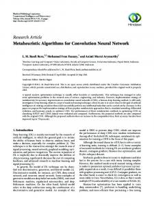
in converging to the optimal MSE whereas BRNN achieved better R2 (see Fig.1a ) than the other
230
learning algorithms. These results indicated that the performance of the algorithms in predicting
231
HTO is not consistent because it depends on the performance metrics being considered as the
232
criteria for measuring performance. Though, in this case LMNN can be chosen despite not
233
having the highest R2 due to its ability to achieve the lowest MSE in the shortest possible time.
234
Seven (7) hidden neurons produce the best MSE result, whereas six (6) hidden neurons is the
235
fastest architecture.
CITATION: Chiroma, H., Abdul-Kareem, S., Muaz, S. A., Khan, A., Sari, E. N., & Herawan, T. (2014). Neural Network Intelligent Learning Algorithm for Inter-related Energy Products Applications. In Advances in Swarm Intelligence (pp. 284-293). Springer International Publishing. 236
Table 5 Comparison of KTJF predicted by NNs learning algorithms models
237 238
Learning Method
LMNN
Performance
Convergence speed
Number of hidden neurons
Number of hidden neurons
4-8-1
4-7-1
4-6-1
4-8-1
4-7-1
4-6-1
0.102(0.8771)
0.0873(0.9245)
0.1(0.88)
47(5)
110(9)
54(2)
1000
1000
1000
3.2(-0.67)
(183)
(168)
(142)
0.29(0.72)
12(2)
16(2)
31(10)
1000
1000
1000
(28)
(27)
(28)
322
531
443
(40)
(49)
(33)
SCGNN
1.3000(-0.4111)
34.3000(-0.7662)
GDANN
0.62(0.7482)
0.744(-0.7108)
BNN
BRNN
15.7(-0.5972)
29(0.7396)
0.0896(0.9108)
13.6(0.68)
0.0896(0.91468)
0.098(0.9)
239 240
The results of the prediction of KTJF price are reported in Table 5, the LMNN has the minimum
241
MSE and the highest R2 (see Fig.1b) among the comparison algorithms. The other algorithms
242
such as BRNN, GDANN (4-8-1, 4-6-1) also have competitive values of MSE and R2 compared
243
to the optimal values. The fastest algorithm is GDANN having the minimum iterations and time
244
of convergence. The performance criteria’s indicated that the LMNN is the best in terms of MSE
245
and R2 whereas convergence speed criteria’s shows GDANN outperforms other algorithms.
246
Seven (7) hidden neurons yield the best MSE and R2 but, the fastest architecture is having eight
247
(8) hidden neurons. This is surprising as less complex structure is expected to be the fastest.
248 249 250 251
Table 6 The comparison of the NNs learning algorithms in the prediction of NYGSL
252 Performance
Convergence speed
Number of hidden neurons
Number of hidden neurons
Learning Method 4-8-1
4-7-1
4-6-1
4-8-1
4-7-1
4-6-1
LMNN
0.0044(0.9983)
0.00158(0.9988)
0.00195(0.9987)
39(3)
60(3)
35(1)
SCGNN
1(-0.1631)
18.6(0.4774)
13.5(0.9531)
1000(183)
1000(153)
1000(141)
GDANN
3.22(0.8825)
2.12(0.8311)
0.490(0.9471)
1(0)
1(0)
1(0)
CITATION: Chiroma, H., Abdul-Kareem, S., Muaz, S. A., Khan, A., Sari, E. N., & Herawan, T. (2014). Neural Network Intelligent Learning Algorithm for Inter-related Energy Products Applications. In Advances in Swarm Intelligence (pp. 284-293). Springer International Publishing. BNN
13(-0.5668)
5.22(0.9338)
0.864(0.8711)
BRNN
0.000025(0.9989)
0.0000279(0.9988)
1000(27)
1000(25)
1000(24)
0.000512(0.9988) 433(48) Training: R=0.91249
954(87)
604(44)
Validation: R=0. 4
Data Fit Y=T
Output ~= 0.83*Target + 0.17
4
Output ~= 0.84*Target + 0.16
253 254
3.5 R=0.99637 price are reported Test: R=0.99568GDANN as the The results of the predictionTraining: of NYGSL in Table 6, showing 4 3
255
Fit 3.5 Fitlearning algorithm with2.5 fastest algorithm to converge to its optimal solution. The BRNN 3.5 2.5
256
2 different architecture is3 the best predictor with the lowest MSE and the highest R2 (see Fig.1c) 2
257
among the comparison 2algorithms.
2.5
1.5 1
1.5
0.5 1
1
3
3
Training: R=0.99904 Data Fit Y=T
20.5 1
2
1.5
3
4
Target
b
1
4.5
Data Fit Training: Y=T
4 3.5 1.8 3 1.6 2.5 1.4 2 1.2 1.5
1
2
Target 1
1.5
2
3
3.5
0.8 0.5 1
2
4.5
R=0.9846
Data Fit Y=T
3 2.5
3
4
0.2 0.5
Data Fit Y=T
4 3.5 3 2.5
Validation Data Fit Y=T
1.8 1.6 1.4
2
1.2
1.5
1
1 0.5
2
Target 1.5
0.4
4
All: R=0.9144
Test: R=0.99845
1 1
0.6
2.5
Target
0.8 0.6 1
2
3
Target
0.4 0.2
1
1
1.5
0.5
Target
Ta
0.5 1
1.5
2
2.5
3
3.5
0.5
Target
Predicted PPN by LMNN
All: R=0.99895 3.5
Data Fit Y=T
3 2.5 2 1.5 1 0.5
Data Fit Y=T
1.8 1.6 1.4 1.2 1 0.8 0.6 0.4 0.2
1
1.5
2
2.5
3
3.5
1
Target
Target
d
1.5
2
2.5
3
Target
All: R Data Fit Y=T
1.8 1.6 1.4 1.2 1 0.8 0.6 0.4 0.2
0.5 0.5
1
Test: R=0.98502
Output ~= 0.97*Target + 0.021
0.5
Predicted NYGSL by BRNN
1
4
Data Fit Y=T
0.5
c
3
0.5
LMNN
Data Fit Y=T
2.5 1
a
1.5
0.5 1
Test: R=0.92453
+ 0.021 ~= 0.97*Target OutputPredicted by KTJF
+ 0.0024 Output ~= 1*Target HTO predicted
by BRNN
4 3.5
31.5
1.5
4
Output ~= 1*Target + 0.002
2
All: R=0.99627
2
2
2
Target
2.5
2.5
0.5
1
3.5
Y=T
3
Target
0.5
260
Data
Output ~= 0.83*Target + 0.17
259
Y=T
3
Output ~= 0.96*Target + 0.026
258
Data
Output ~= 0.99*Target + 0.0099
Output ~= 0.99*Target + 0.0092
4
Data Fit Y=T
3.5
1.5
0.5
1
Ta
Output ~=
Output ~=
2 1.5
2 1.5
Predicted USCGSL by BRNN
1 CITATION: Chiroma, H., Abdul-Kareem,1 S., Muaz, S. A., Khan, A., Sari, E. N., & Herawan, T. 0.5 0.5 (2014). Neural Network Intelligent Learning Algorithm for Inter-related Energy Products 1 2 3 4 1 2 3 Applications. In Advances in Swarm Intelligence (pp. 284-293). Springer International Target Target Publishing.
All: R=0.99825 Data Fit Y=T
4.5 4 3.5 3 2.5 2 1.5 1 0.5 1
2
3
4
Target
e 261
Fig. 1 Regression plots
262 263 264 265 266
SCGNN and GDANN are having the poorest values of MSE despite GDANN has a competitive
267
R2 compared to the promising R2 value of BRNN, LMNN, BNN (4-7-1, 4-6-1), and SCGNN (4-
268
6-1). In the prediction of NYGSL, the performance exhibited a similar phenomenon to the
269
prediction of HTO and KTJF as consistency is not maintained. In the prediction of the NYGSL
270
we cannot conclude on the best algorithms because the performance exhibited by the algorithms
271
is highly random unlike the case in the prediction of HTO. The BRNN converged to the MSE
272
and R2 very slow compared to the LMNN, and GDANN speed. The optimal algorithm in this
273
situation depends on the criteria chosen as the priority in selecting the best predictor. If accuracy
274
is the priority, then BRNN can be the best candidate, whereas speed place LMNN above BRNN.
275
Seven (7) hidden neurons have the best MSE value, whereas the architectures with six (6), seven
276
(7), and eight (8) hidden neurons are the fastest. This could probably be caused by memorizing
277
the training data by the algorithms.
278 279
Table 7 Results ontain with NNs learning algorithms in the prediction of PPN
280 Performance Learning Method
LMNN
Convergence speed
Number of hidden neurons
Number of hidden neurons
4-8-1
4-7-1
4-6-1
4-8-1
4-7-1
4-6-1
0.00514(0.9850)
0.00694(0.9801)
0.00623(0.9820)
74(8)
32(2)
60(4)
4
CITATION: Chiroma, H., Abdul-Kareem, S., Muaz, S. A., Khan, A., Sari, E. N., & Herawan, T. (2014). Neural Network Intelligent Learning Algorithm for Inter-related Energy Products Applications. In Advances in Swarm Intelligence (pp. 284-293). Springer International Publishing. 1000
1000
1000
SCGNN
0.266(-0.4121)
0.646(-0.8601)
0.686(-0.8592)
(179)
(149)
(136)
GDANN
1.78 (-0.8164)
2.45 (-0.2453)
3.31 (0.7886)
1(0)
1(0)
1(0)
1000
1000
1000
BNN
0.276(-0.28011)
0.211(0.3802)
1.62(-0.4091)
(26)
(25)
(25)
BRNN
0.000512(0.984)
0.00557(0.98231)
0.686(-0.8592)
204(19)
226(21)
385(28)
281 282 283
Table 7 indicated that GDANN is the fastest to predict PPN price, whereas the MSE of BRNN is the
284
best. The R2 (see Fig.1d) value of LMNN is the highest compared to the SCGNN, GDANN, BNN, and
285
BRNN R2 values. The performance exhibited by the algorithms in the prediction of PPN price is not
286
different from that of NYGSL, KTJF, and HTO because consistent performance is not realized. The best
287
algorithm for the prediction of PPN price depends on the performance metrics considered as priority for
288
selecting the optimal algorithm as earlier explained. The algorithms with negative values of R2 reported
289
in Tables 4 to 7 suggested that the observed price and the predicted once are in opposite directions.
290
Signifying that upward movement of predicted price can influence the observed price to move
291
downward and vice-versa. This is not true considering the promising results obtained by other
292
algorithms that show positive R2 values.
293
CITATION: Chiroma, H., Abdul-Kareem, S., Muaz, S. A., Khan, A., Sari, E. N., & Herawan, T. (2014). Neural Network Intelligent Learning Algorithm for Inter-related Energy Products Applications. In Advances in Swarm Intelligence (pp. 284-293). Springer International Publishing.
Table 8 Comparison of USGSL predicted by NNs learning algorithms models
294 295
Performance
Convergence speed
Number of hidden neurons
Number of hidden neurons
Learning Method 4-8-1
4-7-1
4-6-1
4-8-1
4-7-1
4-6-1
LMNN
0.00264(0.99821)
0.00330(0.99817)
0.00301(0.99624)
103(7)
21(1)
63(3)
SCGNN
0.00598(0.99686)
0.00403(0.99621)
0.00445(0.99818)
37(1)
146(4)
131(1)
GDANN
0.0531(0.95758)
0.0284(0.97383)
0.0484(0.96635)
55(0)
68(0)
94(1)
BNN
0.0246(0.98191)
0.712(0.69757)
0.913(0.96988)
1000(23)
10(0)
12(0)
BRNN
0.00250(0.99825)
0.00273(0.99785)
0.00235(0.94193)
652(67)
653(57)
563(41)
296 297
In the prediction of USCGSL price as indicated in Table 8, BRNN have the minimum value of
298
MSE and the highest R2 (see Fig.1e), though with a different hidden neurons. The fastest
299
algorithm is the GDANN with seven (7) hidden neurons. It seems hidden layer neurons do not
300
always affect the convergence speed of the NNs algorithms based on experimental evidence
301
from Tables 4 to 8. The results do not deviate from similar behavior shown by the prediction of
302
HTO, PPN, NYGSL, and KTJN prices.
303
Small number of iterations do not necessarily imply lower computational time based on evidence
304
from the simulation results. For example, in Table 8, a GDANN converge to a solution in sixty
305
eight (68) iterations, 0 Sec. Whereas Table 5 indicated that convergence occurs in thirty five (35)
306
iterations, one (1) Sec. with the LMNN which is considered as the most efficient NN learning
307
algorithm in the literature. The poor performance exhibited by some algorithms can be attributed
308
to the possibility that the algorithms could have been trapped in local minima. The complexity of
309
an NNs affects convergence speed as reported in Tables 4 to 8. The fastest architectures have six
310
(6) hidden neurons with exception in the prediction of KTJN. This is a multi tasking experiments
311
perform on the related energy products. We have found from the series of the experiments
312
conducted that the LMNN and BRNN constitute an alternative approaches for predition in the oil
313
market especially when accuracy is the subject of concern. Objective of the research have being
314
achieved since the idle NN learning algorithms were identified for future prediction of the energy
315
products. Therefore, uncertainty related to the oil market can be reduce to the tolerance level
316
which in turn might stabilized the energy product market. The results obtained do not agree with
CITATION: Chiroma, H., Abdul-Kareem, S., Muaz, S. A., Khan, A., Sari, E. N., & Herawan, T. (2014). Neural Network Intelligent Learning Algorithm for Inter-related Energy Products Applications. In Advances in Swarm Intelligence (pp. 284-293). Springer International Publishing. 317
the results reported by [3]. This could probably be attributed to the fair comparison of our study
318
unlike the study by [3] that compared NN and statiscal methods. The results of this study cannot
319
be generalized to other multi-task problems because the performance of NNs learning algorithm
320
depends on the application domain since the NNs performance differ from domain to domain as
321
argued by [28]. However, the methodolopgy can be modified to applied on similar datasets or
322
problem.
323
CONCLUSIONS
324
In this paper, the performance of NNs learning algorithms in energy products price prediction
325
were studied and their performances in terms of MSE, R2, and convergence speed were
326
compared. BRNN was found to have the best result in the prediction of an HTO price in terms of
327
R2 whereas LMNN achieved the minimum MSE and converges faster than the SCGNN,
328
GDANN, BRNN, and BNN in predicting HTO price. In the prediction of KTJF price, LMNN
329
performs better than the SCGNN, GDANN, BRNN, and BNN considers MSE and R 2 as
330
performance criteria’s. In contrast, GDANN is the algorithm to converge faster than the other
331
NNs learning algorithms. On the other hand, prediction of NYGSL is more effective with BRNN
332
in terms of MSE and R2, but GDANN is the fastest. BRNN have the minimum MSE whereas
333
LMNN achieved the maximum R2 in the prediction of PPN price. The fastest among the learning
334
algorithms in the prediction of PPN price is GDANN despite having the poorest MSE values.
335
BRNN performs better than the SCGNN, GDANN, LMNN, and BNN in the prediction of an
336
USCGSL price in terms of MSE and R2. GDANN recorded the best convergence speed
337
compared to SCGNN, BRNN, LMNN, and BNN.
338
The NNs learning algorithms use for the prediction of energy products prices is not meant to
339
replace the financial experts in the energy sector. Perhaps, is to facilitate accurate decision to be
340
taken by decision makers in order to reach better resolutions that could yield profits for the
341
organization. Investors in the energy sector could rely on our study to suggest future prices of the
342
energy products. This can reduce the high level of uncertainty about energy products prices,
343
thereby provide a platform for developmental planning that can result in the improvement of
344
economic standard.
345
CITATION: Chiroma, H., Abdul-Kareem, S., Muaz, S. A., Khan, A., Sari, E. N., & Herawan, T. (2014). Neural Network Intelligent Learning Algorithm for Inter-related Energy Products Applications. In Advances in Swarm Intelligence (pp. 284-293). Springer International Publishing. 346 347
REFERENCES
348 349 350 351 352 353 354 355 356
1. US Department of Energy (2004) Annual Energy Outlook 2004 with Projections to 2025. http://www.eia.doe.gov/oiaf/ archive/aeo04/index.html, Acessed 2014. 2. Malliaris ME, Malliaris SG (2008) Forecasting energy product prices. Eur J Financ 14(6) ,453 – 468. 3. Su F,Wu W (2000) Design and testing of a genetic algorithm neural network in the assessment of gait patterns. Med Eng Phys 22, 67–74. 4. Wang T, Yang J (2010) Nonlinearity and intraday efficiency test on energy future markets. Energ Econ 32, 496 – 503.
357
5. Chen X, Qu Y (2011) A prediction method of crude oil output based on artificial neural
358
networks. In: Proceeding of IEEE International Conference on Computation and Information
359
sciences, Chengdu, China, pp. 702 – 704.
360 361 362 363 364 365 366 367 368 369 370 371 372
6. Shambora WE, Rossiter R (2007) Are there exploitable inefficiencies in the futures market for oil?. Energ Econ 29,18 – 27. 7. Blanco A, Delgado M, Pegalajar MC (2001) A real-coded genetic algorithm for training recurrent neural networks. Neural Networks 14, 93 – 105. 8. Gencay R, Liu T (1997) Nonlinear modeling and prediction with feedforward and recurrent networks. Physica D.108, 119 – 134. 9. Cao L, Tay FEH (2001) Financial forecasting using support vector machines. Neural Comput 10, 184 – 192. 10. Tay FEH, Cao L (2001) Application of support vector machines in financial time series forecasting. Omega 29, 309 – 317. 11. Kulkarni S, Haidar I (2009) Forecasting model for crude oil price using artificial
neural
networks and commodity future prices. Int J Comp Sci Inf Secur 2(1), 81 – 88. 12. Saad WE, Prokhorov VDC, Wunsch CD (1998) Comparative Study of Stock Trend
373
Prediction Using Time Delay, Recurrent and Probabilistic Neural
374
Neural Networ 9(6), 1456 – 1470.
Networks.
IEEE
T
CITATION: Chiroma, H., Abdul-Kareem, S., Muaz, S. A., Khan, A., Sari, E. N., & Herawan, T. (2014). Neural Network Intelligent Learning Algorithm for Inter-related Energy Products Applications. In Advances in Swarm Intelligence (pp. 284-293). Springer International Publishing. 375
13. Fernandez V (2006) Forecasting crude oil and natural gas spot prices by classification
376
methods. IDEAS web
377
http://www.webmanager.cl/prontus_cea/cea_2006/site/asocfile/ASOCFILE12006112810582
378
0.pdf. (2006) , Access 4 January, 2014.
379 380 381 382 383 384 385 386
14. Quek C, Pasquier M, Kumar N (2008) A novel recurrent neural network-based prediction system for option trading and hedging. Appl Intell 29, 138 – 151. 15. Xie W, Yu L, Xu S, Wang S (2006) A new method for crude oil price forecasting
based
on support vector machines. Lect Notes Comput Sci 3994, 441–451. 16. Kaynar O, Yilmaz I, Demirkoparan F (2011) Forecasting of natural gas consumption with neural networks and neuro fuzzy system. Energy Educ Sci Tech 26(2), 221 – 238. 17. Zimberg B (2008) Crude oil price forecasting with ANFIS. University of Vaasa [Online]: web.http://lipas.uwasa.fi/~phelo/ICIL2008TelAviv/24.pdf. Accessed 3 July 2013.
387
18. Qi Y, Zhang W (2009) The improved SVM for forecasting the fluctuation of international
388
crude oil prices. In: Proceedings of IEEE International Conference on Electronic Commerce
389
and Business Intelligence,pp. 269 – 271.
390
19. Yu L, Wang S, Wen B (2008) An AI-agent trapezoidal fuzzy ensemble forecasting model for
391
crude oil prediction. In: proceeding of the IEEE 3rd International Conference on Innovative
392
Computing Information and Control, Dalian, China, doi:10.1109/ICICIC, 124.
393
20. Byvatov E, Fechner U, Sadowski J, Schneider G (2003) Comparison of support vector
394
machine and artificial neural networks for drug/Nondrug classification. J Chem Inf Comput
395
Sci 43, 1882-1889.
396 397 398 399
21. Chen S, Yu P, Liu B (2011). Comparison of neural network architectures and inputs for radar rainfall adjustment for typhoon events. J Hydrol 405, 150–160. 22. Zweiri YH, Whidborne JF, Sceviratne LD (2002) A three-term backpropagation algorithm. Neurocomputing 50, 305–318.
400
23. Haykin S (1999) Neural networks. New Jersey: Prentice Hall, 2nd edn.
401
24. Jammazi R, Aloui C (2012) Crude oil forecasting: experimental evidence from wavelet
402 403 404
decomposition and neural network modeling. Energ Econ 34, 828 – 841. 25. Hair FJ, Black WC, Babin JB, Anderson RE (2010) Multivariate data analysis. New Jersey: Pearson Prentice Hall.
CITATION: Chiroma, H., Abdul-Kareem, S., Muaz, S. A., Khan, A., Sari, E. N., & Herawan, T. (2014). Neural Network Intelligent Learning Algorithm for Inter-related Energy Products Applications. In Advances in Swarm Intelligence (pp. 284-293). Springer International Publishing. 405 406
26. Hornik K (1991) Approximation capabilities of multilayer feedforward networks. Neural Netw 4, 251—257.
407
27. Berry MJA, Linoff G (1997) Data mining techniques. New York: Willey.
408
28. Azar AT (2013) Fast neural network learning algorithms for medical applications. Neural
409 410
Comp Appl 23(3-4), 1019-1034.