embedded systems development in which software interacts with a phys- ... Hybrid systems modeling languages allow models to include both software and.
A Synchronous-based Code Generator For Explicit Hybrid Systems Languages? Timothy Bourke1,3 , Jean-Louis Cola¸co2 , Bruno Pagano2 , C´edric Pasteur2 , and Marc Pouzet4,3,1 1
2
4
INRIA Paris-Rocquencourt ANSYS/Esterel-Technologies, Toulouse 3 ´ DI, Ecole normale sup´erieure, Paris Universit´e Pierre et Marie Curie, Paris
Abstract. Modeling languages for hybrid systems are cornerstones of embedded systems development in which software interacts with a physical environment. Sequential code generation from such languages is important for simulation efficiency and for producing code for embedded targets. Despite being routinely used in industrial compilers, code generation is rarely, if ever, described in full detail, much less formalized. Yet formalization is an essential step in building trustable compilers for critical embedded software development. This paper presents a novel approach for generating code from a hybrid systems modeling language. By building on top of an existing synchronous language and compiler, it reuses almost all the existing infrastructure with only a few modifications. Starting from an existing synchronous data-flow language conservatively extended with Ordinary Differential Equations (ODEs), this paper details the sequence of source-tosource transformations that ultimately yield sequential code. A generic intermediate language is introduced to represent transition functions. The versatility of this approach is exhibited by treating two classical simulation targets: code that complies with the FMI standard and code directly linked with an off-the-shelf numerical solver (Sundials CVODE). ´lus compiler and The presented material has been implemented in the Ze the industrial Scade Suite KCG code generator of Scade 6.
1
Introduction
Hybrid systems modeling languages allow models to include both software and elements of its physical environment. Such models serve as references for simulation, testing, formal verification, and the generation of embedded code. Explicit hybrid systems languages like Simulink/Stateflow5 combine Ordinary Differential Equations (ODEs) with difference and data-flow equations, hierarchical automata in the style of Statecharts [15], and traditional imperative features. ?
5
´lus and the extension of Scade 6 with hybrid features are available Examples in Ze at http://zelus.di.ens.fr/cc2015/. http://mathworks.org/simulink
Models in these languages mix signals that evolve in both discrete and continuous time. While the formal verification of hybrid systems has been extensively studied [8], this paper addresses the different, but no less important, question of generating sequential code (typically C) for efficient simulations and embedded real-time implementations. Sequential code generation for synchronous languages [5] like Lustre [14] has been extensively studied. It can be formalized as a series of source-to-source and traceable transformations that progressively reduce high-level programming constructs, like hierarchical automata and activation conditions, into a minimal data-flow kernel [10]. This kernel is further simplified into a generic intermediate representation for transition functions [6], and ultimately turned into C code. Notably, this is the approach taken in the Scade Suite KCG code generator of Scade 66 , which is used in a wide range of critical embedded applications. Yet synchronous languages only manipulate discrete-time signals. Their expressiveness is deliberately limited to ensure determinacy, execution in bounded time and space, and simple, traceable code generation. The cyclic execution model of synchronous languages does not suffer the complications that accompany numerical solvers. Conversely, a hybrid modeling language allows discrete and continuous time behaviors to interact. But this interaction together with unsafe constructs, like side effects and while loops, is not constrained enough, nor specified with adequate precision in tools like Simulink/Stateflow. It can occasion semantic pitfalls [9,4] and compiler bugs [1]. A precise description of code generation, that is, the actual implemented semantics, is mandatory in safety critical development processes where target code must be trustworthy. Our aim, in short, is to increase the expressiveness of synchronous languages without sacrificing any confidence in their code generators. Benveniste et al. recently proposed a novel approach for the design and implementation of a hybrid modeling language that reuses synchronous language principles and an existing compiler infrastructure. They proposed an ideal synchronous semantics based on non standard analysis [4] for a Lustre-like language with ODEs [3], and then extended the kernel language with hierarchical automata [2] and a modular causality analysis [1]. These results form the founda´lus [7]. This paper describes their validation in an industrial compiler. tion of Ze Paper Contribution and Organisation Our first contribution is to precisely describe the translation of a minimal synchronous language extended with ODEs into sequential code. Our second contribution is the experimental validation in ´lus [7] and the Scade Suite two different compilers: the research prototype Ze KCG code generator. In the latter it was possible to reuse all the existing infrastructure like static checking, intermediate languages, and optimisations, with little modification. The extensions for hybrid features require only 5% additional lines of code. Moreover, the proposed language extension is conservative in that regular synchronous functions are compiled as before—the same synchronous code is used both for simulation and for execution on target platforms. 6
http://www.esterel-technologies.com/products/scade-suite/
time stops
[r e i
tempus fugit
nit]
D
C
even
t
encore
approximate
Fig. 1. Basic structure of a hybrid simulation algorithm
The paper is organised as follows. Section 2 recalls the classical simulation loop of hybrid systems. Section 3 describes the overall compiler architecture as implemented in KCG. Section 4 defines the input language, Section 5 defines a clocked intermediate language, and Section 6 defines the target imperative language. Code generation is defined in Section 6.1. We illustrate the versatility of the compiler in two typical practical situations: generating code that complies with the FMI standard and generating code that incorporates an off-the-shelf ´lus numerical solver (Sundials CVODE). Practical experiments in KCG and Ze are presented in Section 7. Section 8 discusses extensions and related work. We conclude in Section 9.
2
The Simulation Loop of Hybrid Systems
The first choice to make in implementing a hybrid system is how to solve ODEs. Creating an efficient and numerically accurate numerical solver is a daunting and specialist task. Reusing an existing solver is more practical, with two possible choices: either (a) generate a Functional Mock-Up Unit (FMU) using the standardized Functional Mock-Up Interface (FMI) and rely on an existing simulation infrastructure [19]; or (b) use an off-the-shelf numerical solver like CVODE [16] and program the main simulation loop. The latter corresponds to the co-simulation variant (CS) of FMI, where each FMU embeds its own solver. The simulation loop of a hybrid system is the same no matter which option is chosen. It can be defined formally as a synchronous function that defines four streams t(n), lx (n), y(n), and z(n), with n ∈ N. t(n) ∈ R is the increasing sequence of instants at which the solver stops.7 lx (n) is the value at time t(n) of the continuous state variables, that is, of all variables defined by their derivatives in the original model. y(n) is the value at time t(n) of the discrete state. z(n) indicates any zero-crossings at instant t(n) on signals monitored by the solver, that is, any signals that become equal to or pass through zero. The synchronous function has two modes: the discrete mode (D) contains all computations that may change the discrete state or that have side effects. The continuous mode (C) is where ODEs are solved. The two modes alternate according to the execution scheme summarized in Figure 1. 7
In Simulink, these are called major time steps.
The Continuous Mode (C). In this mode, the solver computes an approximation of the solution of the ODEs and monitors a set of expressions for zero-crossings. Code generation is independent of the actual solver implementation. We abstract it by introducing a function solve(f )(g) parameterized by f and g where: – x0 (τ ) = f (y(n), τ, x(τ )) defines the derivatives of continuous state variables x at instant τ ∈ R; – upz(τ ) = g(y(n), τ, x(τ )) defines the current values of a set of zero-crossing signals upz, indexed by i ∈ {1, . . . , k}. The continuous mode C computes four sequences s, lx , z and t such that: (lx , z, t, s)(n + 1) = solve(f )(g)(s, y, lx , t, step)(n) where s(n)
is the internal state of the solver at instant t(n) ∈ R. Calling solve(f )(g) updates the state to s(n + 1).
x
is an approximation of a solution of the ODE, x0 (τ ) = f (y(n), τ, x(τ )) It is parameterized by the current discrete state y(n) and initialized at instant t(n) with the value of lx (n), that is, x(t(n)) = lx (n).
lx (n+1) is the value of x at t(n + 1), that is: lx (n + 1) = x(t(n + 1)) lx is a discrete-time signal whereas x is a continuous-time signal. t(n + 1) is bounded by the horizon t(n) + step(n) that the solver has been asked to reach, that is: t(n) ≤ t(n + 1) ≤ t(n) + step(n) z(n + 1) signals any zero-crossings detected at time t(n + 1). An event occurs with a transition to the discrete mode D when horizon t(n) + step(n) is reached, or when at least one of the zero-crossing signals upz(i), for i ∈ {1, . . . , k} crosses zero,8 which is indicated by a true value for the corresponding boolean output z(n + 1)(i). event = z(n + 1)(0) ∨ · · · ∨ z(n + 1)(k) ∨ (t(n + 1) = t(n) + step(n)) If the solver raises an error (for example, a division by zero or an inability to find a solution), we consider that the simulation fails. 8
The function solve(f )(g) abstracts from the actual implementation of zero-crossing detection. To account for a possible zero-crossing at the horizon t(n) + step(n), the solver may integrate over a strictly larger interval [t(n), t(n) + step(n) + margin], where margin is a solver parameter. z(n + 1)(i) =
(∀T ∈ [t(n), t(n + 1)[ . upz(T )(i) < 0) ∧ ∃m ≤ margin . (∀T ∈ [t(n + 1), t(n + 1) + m] . upz(T )(i) ≥ 0)
This definition assumes that the solver also stops whenever a zero-crossing expression passes through zero from positive to negative.
The Discrete Mode (D). All discrete changes occur in this mode. It is entered when an event is raised during integration. During a discrete phase, the function next defines y, lx , step, encore, z, and t: (y, lx , step, encore)(n + 1) = next(y, lx , z, t)(n) z(n + 1) = false t(n + 1) = t(n) where y(n + 1)
is the new discrete state; outside of mode D, y(n + 1) = y(n).
lx (n + 1)
is the new continuous state, which may be changed directly in the discrete mode.
step(n + 1)
is the new step size.
encore(n+1) is true if an additional discrete step must be performed. Function next can decide to trigger instantaneously another discrete event causing an event cascade [4]. t(n)
(the simulation time) is unchanged during discrete phases.
The initial values for y(0), lx (0) and s(0) are given by an initialization function init. Finally, solve(f )(g) may decide to reset its internal state if the continuous state changes. If init solve(lx (n), s(n)) initializes the solver state, we have: reinit = (lx (n + 1) 6= lx (n)) s(n + 1) = if reinit then init solve(lx (n + 1), s(n)) else s(n) Taken together, the definitions from both modes give a synchronous interpretation of the simulation loop as a stream function that computes the sequences lx , y and t at instant n + 1 according to their values at instant n and an internal state. Writing solve(f )(g) abstracts from the actual choice of integration method and zero-crossing detection algorithm. A more detailed description of solve(f )(g) would be possible (for example, an automaton with two states: one that integrates, and one that detects zero-crossings) but with no influence on the code generation problem which must be independent of such simulation details. Given a program written in a high-level language, we must produce the functions init, f , g, and next. In practice, they are implemented in an imperative language like C. Code generation for hybrid models has much in common with code generation for synchronous languages. In fact, the following sections show how to extend an existing synchronous language and compiler with ODEs.
3
Compiler Architecture
The compiler architecture for hybrid programs is based on those of existing compilers for data-flow synchronous languages like Scade 6 or Lucid Synchrone,
parsing
typing
causality
control encoding
optimization
C code generation
dead-code removal
slicing
SOL generation
scheduling
Fig. 2. Compiler architecture (modified passes are gray; new ones are also dashed)
as described for instance in [6]. After initial checks, it consists in successive rewritings of the source program into intermediate languages, and ending with sequential code in the target language (typically C). The different passes are shown in Figure 2: 1. Parsing transforms code in the source language, described in Section 4, into an abstract syntax tree; 2. Typing checks programs according to the system of [3]. In the language extended with ODEs, this system distinguishes continuous and discrete blocks to ensure the correct separation of continuous and discrete behaviors; 3. Causality analysis verifies the absence of causality loops [1]. It is readily extended to deal with the new constructs; 4. Control structures are encoded into the purely data-flow kernel with clocks defined in Section 5, using an extension of the clock-based compilation of [6]. A small modification accounts for the fact that transitions are executed in a discrete context whereas the bodies of states are continuous; 5. Traditional optimizations (dead-code removal, common sub-expression elimination, etc.) are performed; 6. Scheduling orders equations according to data dependencies, as explained in Section 5.2; 7. Code is translated into an intermediate sequential object language called SOL, defined in Section 6 together with the translation. This language extends the one presented in [6] to deal with the new constructs (continuous states, zero-crossings) which translation to sequential code must be added; 8. Slicing specializes the sequential function generated for each node into functions f , g, and next, as described in Section 6.2; 9. Dead-code removal eliminates useless code from functions. For instance, derivatives need not be computed by the next function and values of zerocrossings are surely false during integration; 10. The sequential code is translated to C code. The compiler passes in gray in Figure 2 are those that must be modified in, or added to (dashed borders), a traditional synchronous language compiler. The modifications are relatively minor—around 10% of each pass—and do not require major changes to the existing architecture. Together with the new passes, they amount to 5% of the total code size of the compiler.
d ::= let x = e | let k f (pi) = pi where E | d; d e ::= x | v | op(e, . . . , e) | pre(e) | e -> e | last x | f (e, . . . , e) | (e, . . . , e) | up(e) p ::= x | (x, . . . , x) pi ::= xi | xi, . . . , xi xi ::= x | x last e | x default e E ::= p = e | der x = e | if e then E else E | present e then E else E | reset E every e | local pi in E | do E and . . . E done k ::= D | C | A Fig. 3. A synchronous kernel with ODEs
4
A Synchronous Language Kernel with ODEs
We consider a synchronous language extended with control structures and ODEs. The synchronous sub-language, that is, with ODEs removed, is the subset of ´lus [7], the language considered Scade 6 [13] described in [10]. Compared to Ze here does not include hierarchical automata, but they can be translated into the presented kernel [2]. The abstract syntax given in Figure 3 is distilled from the two concrete languages on which this material is based. A program is a sequence of definitions (d), of either a value (let x = e) that binds the value of expression e to x, or a function (let k f (pi ) = pi where E). In a function definition, k is the kind of the function f , pi denotes formal parameters, and the result is the value of an expression e which may contain variables defined in the auxiliary equations E. There are three kinds: k = A (omitted in the concrete syntax) signifies a combinational function like, for example, addition; k = D (written node in the concrete syntax) signifies a function that must be activated at discrete instants (typically a Lustre or Scade node); k = C (written hybrid in the concrete syntax) signifies a function that may contain ODEs and which must be activated in continuous-time. An expression e is either a variable (x), an immediate value (v), for example, a boolean, integer or floating point constant, the point-wise application of an imported function (op) like +, ∗, or not(·), an uninitialized delay (pre(e)), an initialization (e1 -> e2 ), the previous value of a state variable (last x), a function application (f (e)), a tuple (e, . . . , e) or a rising zero-crossing detection (up(e)). A pattern p is a list of identifiers. pi is a list of parameters where a variable x can be assigned a default value e (x default e) or declared as a state initialized with e (x last e). An equation (E) is either an equality between a pattern and an expression which must hold at every instant (p = e); the definition of the current derivative of x (der x = e); a conditional that activates a branch according to the value of a boolean expression (if e then E1 else E2 ), or a variant that operates on event expressions (present e then E1 else E2 ); a reset on a condition e (reset E every e); a localization of variables (local xi in E); or a synchronous composition of zero or more equations (do E and . . . E done).
In this language kernel, a synchronous function taking input streams tick and res, and returning the number of instants when tick is true, reset every time res is true, is written: ♣9 let node counting(tick, res) = o where reset local c last 0 in do if tick then do c = last c + 1 done and o = c done every res
The if/then abbreviates a conditional with an empty else branch. c is declared to be a local variable initialized to 0 (the notation is borrowed from Scade 6). Several streams are defined in counting such that ∀n ≥ 0, o(n) = c(n) with: 1. (last c)(0) = 0 and ∀n > 0, last c(n) = if res(n) then 0 else c(n − 1) 2. c(n) = if tick(n) then last c(n) + 1 else last c(n) The node keyword (k = D) in the definition signals that this program is purely synchronous. As a first program in the extended language we write the classic ‘bouncing ball’ program with a hybrid (k = C) declaration: ♣ let hybrid bouncing(y0, y’0) = (y last y0) where local y’ last y’0 in do der y = y’ and present up(-. last y) then do y’ = -0.8 *. last y’ done else do der y’ = -. g done
where g is a global constant for gravity. Given initial position y0 and speed y’0, this program returns the current position y. The derivative of y’ is −g and y’ is reset to −0.8 · last y 0 when last y 0 , the left-limit of the signal y, becomes zero. In the following, we suppose that programs have passed the static checking defined in [3] and that they are causally correct [1].
5
A Clocked Data-flow Internal Language
We now introduce the internal clocked data-flow language into which the input language is translated. Its syntax is defined in Figure 4. Compared to the previous language, the body of a function is now a set of equations of the form (xi = ai )xi ∈I where the xi are pairwise distinct variables and each ai is an expression e annotated with a clock ck : e is only evaluated when the boolean formula ck evaluates to true. The base clock is denoted base; it is the constant true. ck on a is true when both ck and a are true. An expression eck with clock ck = (base on a1 · · · ) on an is evaluated only when for all 1 ≤ i ≤ n, ai is true. An expression e is either a variable (x), an immediate value (v), the application of an operator (op(a, . . . , a)), the i-th element of a tuple a (get(a, i)), a delay 9
The ♣’s link to http://zelus.di.ens.fr/cc2015/, which contains both examples ´lus and Scade hybrid, and the C code generated by the latter’s compiler. in Ze
d ::= let x = c | let k f (p) = a where C | d; d a ::= eck e ::= x | v | op(a, . . . , a) | get(a, i) | v fby a | pre(a) | integr(a, a) | f (a, . . . , a) every a | (a, . . . , a) | up(a) | merge(a, a, a) | a when a p ::= x | (x, . . . , x) C ::= (xi = ai )xi ∈I ck ::= base | ck on a k ::= D | C | A Fig. 4. A clocked data-flow internal language
initialized with a constant (v fby a), an uninitialized delay (pre(a)), an integrator whose derivative is a1 and whose output is a2 (integr(a1 , a2 )), a function application reset when a signal a is true (f (a1 , . . . , an ) every a), an n-tuple of values (a1 , . . . , an ), the zero-crossing detection operator (up(a)), the combination of signals a1 and a2 according to the boolean signal a (merge(a, a1 , a2 )), or a signal a1 sampled on condition a2 (a1 when a2 ), This clocked internal representation is a Single Static Assignment (SSA) representation [11]. Every variable x has a single definition and the clock expression defines when it is computed. The main novelty with respect to the clocked internal language of [6] is the introduction of operators integr(a1 , a2 ) and up(a). 5.1
Translation
The translation from a synchronous data-flow language with the control structures if/then/else, present/else and reset/every into clocked data-flow equations is defined in [10]. The Scade Suite KCG code generator follows the same algorithm. We illustrate the translation on three kinds of examples. Translation of Delays and Conditionals. In the example below, z is an input, x1 and x2 are local variables, and the last value of x1 is initialized with 42: local x1 last 42, x2 in if z then do x1 = 1 + last x1 and x2 = 1 + (0 fby (x2 + 2)) done else do x2 = 0 done The translation of the above program returns the following set of clocked equations. To simplify the notation, we only expose the clocks of top-level expressions. x1 = merge(z, 1 + (m1 when z), m1 when not(z)) m1 = (42 fby x1 )
base base
x2 = merge(z, 1 + m2 , 0)
m2 = (0 fby ((x2 when z) + 2))
base on z
base
In this translation, the conditional branch for when z is false is implicitly completed with the equation x1 = last x1 , that is, x1 is maintained. The value of last x1 is stored in m1 . It is the previous value of x1 on the clock where x1 is defined: here, the base clock. The initialized delay 0 fby x2 is local to a branch, and thus equal to the last value that was observed on x2 . This observation is made only when z is true, that is, when clock base on z is true. Translation of Nested Resets. The second example illustrates the translation of the reset construct and its effect on unit delays. reset if c then do x1 = 1 else x1 = (0 fby x1 ) + 1 done reset x2 = (1 fby x2 ) + 1 every k2 every k1 The condition of a reset is propagated recursively to every stateful computation within the reset. This is the case for unit delays and applications of stateful functions. The above program is first translated into: x1 = merge(c, 1, m1 + 1) x2 = (m2 + 1)
base
base base on not(c)
m1 = (0 fby x1 )
base
m2 = (1 fby x2 )
every k1 base
every k1 base or k2 base
base on not(c)
The notation (0 fby x1 ) every k1 base defines the sequence m1 whose value is reset to 0 every time k1 is true. Resets of unit delays are translated into regular clocked equations. We replace the equations for m1 and m2 with: m1 = merge(k1 , 0, r1 when not(k1 ))
base base
r1 = (0 fby merge(c, m1 when c, x1 when not(c))) m2 = merge(k1 , 1, merge(k2 , 1, r2 ) when not(k1 ))
base
base
r2 = (1 fby x2 )
Translation of Integrators. The bouncing ball program from Section 4 becomes: base
y = (y0 -> ly)
ly = integr(y 0 , y)
base
ly 0 = integr(t1 , y 0 )
base
y 0 = merge(z, −0.8∗.ly 0 when z, ly 0 when not(z)) base
t1 = merge(z, 0.0, −.g) base
z = up(−. ly)
base
The variable y 0 changes only when z is true and keeps its last value ly 0 otherwise. The operation integr(a1 , a2 ) defines a signal as the integration of a1 in the continuous mode (C) and as a2 in the discrete mode (D). The derivative of ly 0 is −.g when z is false and otherwise it is 0.0 (constant ly 0 ). 5.2
Static Data-flow Dependencies and Well Formed Schedules
Code is generated in two steps: (a) equations are first statically scheduled according to data-flow dependencies, (b) every equation is translated into an imperative statement in a target sequential language. Data-flow dependencies are defined as in Lustre [14]: an expression a which reads a variable x, must be scheduled after x. The dependency relation is reversed when x is defined by a delay like, for example, x = v fby a1 . In this case a must be scheduled before x. In other words, delays break dependency relations. The integrator x = integr(a1 , a2 ) plays the role of a delay: x does not depend instantaneously on variables in a1 or in a2 , and any read of x must be performed before x is defined. Equations are normalized so that unit delays, integrators, function calls, and zero-crossings appear only at the roots of defining expressions. We partition expressions into three classes: strict (se), delayed (de) and controlled (ce). An expression is strict if its output depends instantaneously on its inputs, otherwise it is delayed. A controlled expression ce is strict. ck
eq ::= x = ce ck | x = f (sa, . . . , sa) every sa | x = de ck sa ::= se ck ca ::= ce ck se ::= x | v | op(sa, . . . , sa) | get(sa, i) | (sa, . . . , sa) | sa when sa ce ::= se | merge(sa, ca, ca) | ca when sa de ::= pre(ca) | v fby ca | integr(ca, ca) | up(ca) A controlled expression is essentially a tree of merge(·, ·, ·) expressions terminated by the application of a primitive, a variable, or a constant. Merges are implemented as nested conditionals. Let Read (a) denote the set of variables read by a. Given a set of normalized equations C = (xi = ai )xi ∈I , a valid schedule Schedule(·) : I → {1 . . . |I|} is a one-to-one function such that, for all xi ∈ I and xj ∈ Read (ai ) ∩ I: 1. if ai is strict, Schedule(xj ) < Schedule(xi ), and, 2. if ai is delayed, Schedule(xi ) ≤ Schedule(xj ). Checking that a given sequence of equations fulfills the well formation rules can be done in polynomial time. Schedules can be obtained by topological sorting but the resulting code is poor. Finding a schedule that minimizes the number of openings and closings of control structures is NP-hard [22]. In the following, if C = (xi = ai )xi ∈I , we suppose the existence of a scheduling function SchedEq(C) that returns a sequence of scheduled equations. We are now ready to define the sequential target language.
md ::= let x = c | let f = classhM, I, (method i (pi ) = ei where Si )i∈[1..n] i | md ; md M
::= [x : m[= v]; . . . ; x : m[= v]]
I
::= [o : f ; . . . ; o : f ]
m
::= Discrete | Zero | Cont
e
::= v | lv | get(e, i) | op(e, . . . , e) | o.method (e, . . . , e) | (e, . . . , e)
S
::= () | lv ← e | S ; S | var x, . . . , x in S | if c then S else S
R, L ::= S; . . . ; S lv
::= x | lv .field | state (x) Fig. 5. A simple object-based language
6
A Sequential Object Language
We define a simple object-based language called SOL to serve as an intermediate language in the translation. It is designed to be easily translatable into target languages like C and Java and resembles the language introduced in [6] and used in KCG. Each stateful function in the source language is translated into a class with an internal memory that a collection of methods act on. The syntax is given in Figure 5. A program is a sequence of constant and class definitions (md). Class definitions take the form classhM, I, (method i (pi ) = ei where Si )i∈[1..n] i and comprise a list M of memories, a list I of instances and a list of methods. A memory entry [x : m[= v]] defines a variable x of kind m, optionally initialized to a constant v. A memory x is either a discrete state variable (Discrete), a zerocrossing (Zero), or a continuous state variable (Cont). An instance entry [o : f ] stores the internal memory of a nested function f . The memories, instances, and methods in a class must be pair-wise distinct. An expression (e) is either an immediate value (v), an access to the value of a variable (lv ), an access to a tuple (get(e, i)), an application of an operation to an argument (op(e, . . . , e)), a method invocation (o.method (e, . . . , e)), or a tuple ((e1 , . . . , en )). An instruction (S) is either void (()), an assignment of the value of e to a left value lv (lv ← e), a sequence (S1 ; S2 ), the declaration of local variables (var x1 , . . . , xn in S), or a conditional (if e then S1 else S2 ). To make an analogy with object-oriented programming, memories are instance variables of a class. The value of a variable x of kind Discrete is read from state (x) and is modified by writing state (x) ← c. Variables x of kind Zero are used to compile up(e) expressions. Each x has two fields: state (x).zin is a boolean set to true only when a zero-crossing on x has been detected, and state (x).zout stores the current value of the expression for monitoring during integration. A variable x of kind Cont is a continuous state variable: state (x).der is its instantaneous derivative and state (x).pos its value. We do not present the translation from SOL to C code (see [6] for details).
6.1
Producing a Single Step Function
We now describe the translation of the clocked internal language into SOL code. Every function definition is translated into a class with two methods: a method reset which initializes the internal memory and a method step which, given an internal memory and current input value, returns an output and updates the internal memory. The translation follows the description given in [6] and implemented in KCG. Here we describe the novelties related to ODEs and zerocrossings. Given an environment ρ, an expression e, and an equation E: – TrExp(ρ)(e) returns an expression of the target language. – TrIn(ρ)(lv)(a) translates a and returns an assignment S that stores the result of a into the left value lv. – TrEq(ρ)(eq) = hI, R, Li translates an equation eq and returns a set of instances I, a sequence of instructions R to be executed at initialization, and a sequence of instructions L to be executed at every step. – TrEq(ρ)(eq 1 · · · eq n ) = hI, R, Li translates sequences of equations eq 1 · · · eq n . An environment ρ associates a name and a kind to every local name in the source program. A name is either a variable (kind Var ) or a memory (kind Mem(m)). We distinguish three kinds of memories: discrete (Discrete), zero-crossing (Zero), and continuous (Cont). Memories can optionally be initialized. ρ ::= [ ] | ρ, x : s
s ::= Var | Mem(m) | Mem(m) = v
The main function translates global definitions of values and functions into global values and classes. It uses auxiliary functions whose definitions follow.10 TrDef (let k f (p) = a where C) = let ρ = Env (C) in let M, (x1 , . . . , xn ) = mem(ρ) in let [eq1 · · · eqn ] = SchedEq(C) in let (hIi , Ri , Li i = TrEq(ρ)(eqi ))i∈[1..n] in let e = TrExp(ρ)(a) in let I = I1 + · · · + In and R = R1 ; . . . ; Rn and L = L1 ; . . . ; Ln in let f = classhM, I, reset = R step(p) = e where var x1 , . . . , xn in Li TrDef (let x = e) = let x = TrExp([ ])(e) First of all, equations in C must conform to the well formation rules defined in Section 5.2. Env (C) builds the environment associated to C and ρ(xi ) defines the kind associated to a defined variable from C: Env ({x1 = a1 , . . . , xn = an }) = Env (x1 = a1 ) + · · · Env (xn = an ) ck
Env (x = pre(a) ) = [x : Mem(Discrete)] ck
Env (x = up(e) ) = [x : Mem(Zero)] ck
Env (x = integr(a1 , a2 ) ) = [x : Mem(Cont)] Env (x = a) = [x : Var ] otherwise 10
The let used in defining the translation function is not the syntactic let of programs.
TrExp(ρ)(v)
=v
TrExp(ρ)(x)
= state(ρ)(x)
TrExp(ρ)(get(a, i))
= get(TrExp(ρ)(a), i)
TrExp(ρ)(op(a1 , . . . , an ))
= let (ci = TrExp(ρ)(ai ))i∈[1..n] in op(c1 , . . . , cn )
TrExp(ρ)((a1 , . . . , an ))
= let (ci = TrExp(ρ)(ai ))i∈[1..n] in (c1 , . . . , cn )
TrExp(ρ)(a1 when a2 )
= TrExp(ρ)(a1 )
TrIn(ρ)(lv )(a1 when a2 )
= TrIn(ρ)(lv )(a1 )
TrIn(ρ)(lv )(merge(a1 , a2 , a3 )) = if TrExp(ρ)(a1 ) then TrIn(ρ)(lv )(a2 ) else TrIn(ρ)(lv )(a3 ) TrIn(ρ)(lv )(a)
= lv ← TrExp(ρ)(a)
otherwise
Fig. 6. The translation function for combinatorial expressions
mem(ρ) returns a pair M, (x1 , . . . , xn ) where M is an environment of memories (kind Mem(m)), and (x1, . . . , xn ) is a set of variables (kind Var ). The set of equations C is statically scheduled with an auxiliary function SchedEq(C). Every equation is translated into a triple hIi , Ri , Li i. The set of instances I1 , . . . , In are gathered, checking that defined names appear only once. Finally, the code associated to f is a class with a set of memories M , a set of instances I and two methods: reset is the initialization method used to reset all internal states, and step is the step function parameterized by p. Given a clock expression ck and an instruction S, Control (ck )(S) returns an instruction that executes S only when ck is true. We write if e then S as a shortcut for if e then S else (). Control (base)(S) = S Control (ck on e)(S) = Control (ck)(if e then S) The translation function for expressions is defined in Figure 6 and raises no difficulties. It uses the auxiliary function state(ρ)(x): state (x) state (x).zin state(ρ)(x) = state (x).pos x
if ρ(x) = Mem(Discrete) if ρ(x) = Mem(Zero) if ρ(x) = Mem(Cont) otherwise
Access to a discrete state variable is written state (x). The current value of a zero-crossing event (kind = Zero) is stored into state (x).zin while the current value of a continuous state variable (kind = Cont) is stored into state (x).pos. The translation function for equations is given in Figure 7:
0
ck
TrEq(ρ)(x = (f (a) every eck ) ) = let (ei = TrExp(ρ)(ai ))i∈[1..n] in 0
let e = TrExp(ρ)(eck ) in let L = Control (ck 0 )(if e then o.reset); Control (ck )(x ← o.step(e1 , . . . , en )) in h[o : f ], o.reset, Li TrEq(ρ)(x = pre(a)ck )
= let S = TrIn(ρ)(state (x))(a) in h[ ], [ ], Control (ck )(S)i
TrEq(ρ)(x = v fby ack )
= let S = TrIn(ρ)(state (x))(a) in h[ ], state (x) ← v, Control (ck )(S)i
TrEq(ρ)(x = integr(a1 , a2 )ck )
= let S1 = TrIn(ρ)(state (x).der )(a1 ) in let S2 = TrIn(ρ)(state (x).pos)(a2 ) in h[ ], [ ], Control (ck )(S1 ; S2 )i
TrEq(ρ)(x = up(a)ck )
= Control (ck )(TrIn(ρ)(state (x).zout)(a))
TrEq(ρ)(x = eck )
= Control (ck )(TrIn(ρ)(state(ρ)(x))(a)) otherwise Fig. 7. The translation function for equations
0
ck
1. The translation of a function application (f (a1 , . . . , an ) every eck ) defines a fresh instance [o : f ]. This instance is reset by calling method o.reset every time ck 0 on e is true. It is activated by calling method o.step when ck is true. 2. A unit delay pre(a) or v fby a is translated into a clocked assignment to a state variable. 3. An integrator is translated into two assignments: one defining the current derivative state (x).der , and the other defining the current value of the continuous state state (x).pos. 4. A zero-crossing is translated into an equation that defines the current value of the signal to observe (state (x).zout).
6.2
Slicing
The translation to SOL generates a step method for each function declaration. Functions declared to be discrete-time (k = D) are regular synchronous functions and they require no additional treatment. But functions declared to be continuous-time (k = C) require specializing the method step to obtain the three functions f , g and next introduced in Section 2: – The next function is obtained by copying the body of step and removing the computation of derivatives, that is, writes to the state (x).der field of
memories of kind Cont, and the computation of zero-crossings, that is, writes to the state (z).zout field of memories of kind Zero. – A method called cont is added to compute the values of derivatives and zero-crossing signals. Functions f and g call this method and then return, respectively, the computed derivatives and the computed zero-crossings. The cont method is obtained by removing all code activated on a discrete clock, that is, by replacing all reads of the state (z).zin fields of memories of kind Zero with false. Indeed, we know that the status z of zero-crossings is always false in the continuous mode C. Writes to the state (x).pos field of memories of kind Cont can also be removed. Finally, all conditions on an event (variables of type zero) are replaced with the value false. The goal of this transformation is to optimize the generated code and to avoid useless computation. The behavior of the generated code is not changed—the code removed, for a given mode, is either never activated or computes values that are never read. Traditional optimizations like constant propagation and dead-code removal can be applied after slicing to further simplify each method. 6.3
Transferring Data to and from a Solver
The transformations described above scatter the values of continuous states and zero-crossings across the memories of the objects that comprise a program. Numerical solvers must able to read and write these memories in order to perform simulations. A simple solution is to augment each object with new methods that copy values to and from the memory fields and arrays provided by a solver. When generating C code, another approach is to define a global array of pointers to the continuous states that can be used to read and write directly to memory ´lus implements the first solution; KCG implements the second. fields. Ze
7 7.1
Practical Experiments Z´ elus with SUNDIALS
´lus is, at its core, essentially the language defined in Section 4. It is compiled Ze into the intermediate language defined in Section 6, which is, in turn, translated directly into OCaml. To produce working simulations, the loop described at a high-level in Section 2 is implemented in two parts: (a) additional methods in the intermediate language, and, (b) a small run-time library. The additional methods derivatives and crossings are specializations of the generated step function that present the interface expected by the runtime library. These functions contain assignments that copy between the vectors passed by a numerical solver and the internal variables described in Section 6.1. Another additional method implements the looping implied by the transition labelled ‘encore’ in Figure 1. It makes an initial step that only updates the internal values of ‘last’ variables, then a discrete step with zero-crossings from the solver, and then further discrete steps, without solver zero-crossings, until
the calculated horizon exceeds the current simulation time. There is a trade-off to make between code generated by the compiler and code implemented in the run-time library. In this case, looping within the generated code allows us to exploit several invariants on the values of internal variables. The run-time library implements the other transitions of Figure 1 and manages numerical solver details. The library declares generic interfaces for ‘state solvers’ and ‘zero-crossing solvers’. The state solver interface comprises functions for initialization, reinitialization, advancing the solution by one step, and interpolating between the last step and the current step. The zero-crossing solver interface includes almost the same functions, but with different arguments, except that interpolation between steps is replaced by a function for finding instants of zero-crossing between two steps. Modules satisfying these two interfaces are combined by generic code to satisfy the ‘solver’ interface described in Section 2. 7.2
SCADE with FMIs
In a second experiment, we extended the Scade Suite KCG code generator of SCADE 6 using the ideas presented in earlier sections. This generator produces a C code instantiation of a ‘Functional Mockup Unit’ (FMU) that respects the FMI for Model Exchange 1.0 standard [19]. An FMU describes a mix of ODEs and discrete events. It is simulated, with or without other components, by an external solver provided by a host. The execution model of FMI [19, Section 2.9] resembles the scheme described in Section 2 and is readily adapted to give the behavior described by Figure 1. The code generated by the compiler is linked to a run-time library which implements the functions required by the FMI standard. There are generic functions to instantiate and terminate the FMU, to enable logging, to set the simulation time, and so on. The implementation of the set function for continuous states (fmiSetContinuousStates), called by the host before an event, copies the given inputs to the corresponding continuous states lx . The get function (fmiGetContinuousStates) returns the new value of lx to the solver after an event. Similar functions exist for inputs, outputs, and zero-crossings (termed event indicators in FMI). At any instant, the first of these set or get functions calls the cont method of the root node; subsequent calls used cached values. In response to a discrete event (fmiEventUpdate), the step method is called once, and then repeatedly while encore(n + 1) is true. For the additional calls, the status of z(n) is computed by comparing the current value of zero-crossing signals with their values after the previous discrete step. The reinit flag, which is set if a continuous state is reset, corresponds to the stateValuesChanged field of the fmiEventInfo input structure of fmiEventUpdate.
8
Discussion and Related Works
This work is related to the definition of an operational semantics for block diagram languages that mix discrete and continuous time behaviors [17]. A unified
semantics is given to PtolemyII [21] in which basic operators are characterized by four atomic step functions that depend on input, internal state, and simulation time and that act on an internal state according to a calling policy [23]. This semantics is modular in the sense that any composition of operators results in the same four functions. It generalizes the operational semantics of explicit hybrid modelers presented in [17] and [12]. The idea that a state transformer can be represented by a collection of atomic functions is much older and has been implemented since the late 1990s in Simulink s-functions11 . It is also the basis of the FMI and FMU standards for model exchange and co-simulation. In our compiler organization, the four functions would correspond to four methods of a SOL machine. The novelty is not the representation of a state transformer as a set of methods but rather the production of those methods in a traceable way that recycles an existing synchronous compiler infrastructure. The result is not an interpreter, as in [23], but a compiler that produces statically scheduled sequential code. The observation that the synchronous model could be leveraged to model the simulation engine of hybrid systems was made by Lee and Zheng [18]. Our contribution is the use of a synchronous compiler infrastructure to effectively build a hybrid modeling language. The present work deliberately avoids considering the early compiler stages that perform static typing and causality analysis. These stages are defined in [3,1] for a similar language kernel. Presented with a program that has not passed static checking and causality analysis, code generation either fails or generates incorrect code. For instance, the equation x = x + 1 cannot be statically scheduled according to Section 5.2 and code generation thus fails. Activating an equation x = 0 -> pre x + 1 in a continuous block would produce imperative code that increments x during integration. ´lus [7] compiled ODEs to purely synchronous code by Previous work on Ze adding new inputs and outputs to each continuous node. For each continuous state, the node takes as input the value computed by the solver and returns the derivative and the new value of the continuous state. We have chosen here to delay this translation to the generation of sequential code. This approach is much easier to integrate into more complex languages like Scade 6 with higherorder constructs like iterators [20]. It also avoids the cost of copying the added arguments at every function call.
9
Conclusion
This full-scale experimental validation confirms the interest of building a hybrid systems modeling language on top of a synchronous language. We were surprised to discover that the extension of Scade 6 with hybrid features required only 5% extra lines of code in total. It confirms the versatility of the compiler architecture of Scade 6, which is based on successive rewritings of the source program into several intermediate languages. 11
http://www.mathworks.com/help/pdf_doc/simulink/sfunctions.pdf
Moreover, while sequential code generation in hybrid modeling tools is routinely used for efficient simulation, it is little used or not used at all to produce target embedded code in critical applications that are submitted to strong safety requirements. This results in a break in the development chain: parts of applications must be rewritten into either sequential or synchronous programs, and all properties verified on the source model cannot be trusted and have to be reverified on the target code. The precise definition of code generation, built on the proven compiler infrastructure of a synchronous language avoids the rewriting of control software and may also increase confidence in simulation results.
Acknowledgments We warmly thank Albert Benveniste and the anonymous reviewers for their helpful remarks on this paper.
References 1. A. Benveniste, T. Bourke, B. Caillaud, B. Pagano, and M. Pouzet. A type-based analysis of causality loops in hybrid systems modelers. In Int. Conf. Hybrid Systems: Computation and Control (HSCC 2014), Berlin, Germany, Apr. 2014. ACM. 2. A. Benveniste, T. Bourke, B. Caillaud, and M. Pouzet. A Hybrid Synchronous Language with Hierarchical Automata: Static Typing and Translation to Synchronous Code. In ACM SIGPLAN/SIGBED Conf. on Embedded Software (EMSOFT’11), Taipei, Taiwan, Oct. 2011. 3. A. Benveniste, T. Bourke, B. Caillaud, and M. Pouzet. Divide and recycle: types and compilation for a hybrid synchronous language. In ACM SIGPLAN/SIGBED Conf. on Languages, Compilers, Tools and Theory for Embedded Systems (LCTES’11), Chicago, USA, Apr. 2011. 4. A. Benveniste, T. Bourke, B. Caillaud, and M. Pouzet. Non-Standard Semantics of Hybrid Systems Modelers. Journal of Computer and System Sciences (JCSS), 78(3):877–910, May 2012. Special issue in honor of Amir Pnueli. 5. A. Benveniste, P. Caspi, S. Edwards, N. Halbwachs, P. Le Guernic, and R. de Simone. The synchronous languages 12 years later. Proc. IEEE, 91(1), Jan. 2003. 6. D. Biernacki, J.-L. Colaco, G. Hamon, and M. Pouzet. Clock-directed modular code generation of synchronous data-flow languages. In ACM Int. Conf. Languages, Compilers and Tools for Embedded Systems (LCTES), Tucson, Arizona, June 2008. 7. T. Bourke and M. Pouzet. Z´elus, a Synchronous Language with ODEs. In Int. Conf. on Hybrid Systems: Computation and Control (HSCC 2013), Philadelphia, USA, Apr. 2013. ACM. 8. L. Carloni, M. D. D. Benedetto, A. Pinto, and A. Sangiovanni-Vincentelli. Modeling Techniques, Programming Languages, Design Toolsets and Interchange Formats for Hybrid Systems. Technical report, IST-2001-38314 WPHS, Columbus Project, Mar. 2004. 9. P. Caspi, A. Curic, A. Maignan, C. Sofronis, and S. Tripakis. Translating DiscreteTime Simulink to Lustre. ACM Trans. on Embedded Computing Systems, 2005. Special Issue on Embedded Software.
10. J.-L. Cola¸co, B. Pagano, and M. Pouzet. A Conservative Extension of Synchronous Data-flow with State Machines. In ACM Int. Conf. on Embedded Software (EMSOFT’05), Jersey city, New Jersey, USA, Sept. 2005. 11. R. Cytron, J. Ferrante, B. K. Rosen, M. N. Wegman, and F. K. Zadeck. Efficiently computing static single assignment form and the control dependence graph. ACM Trans. Program. Lang. Syst., 13(4):451–490, Oct. 1991. 12. B. Denckla and P. Mosterman. Stream and state-based semantics of hierarchy in block diagrams. In Proc. of the 17th IFAC World Congress, pages 7955–7960, 2008. 13. Esterel-Technologies. Scade language reference manual. Technical report, EsterelTechnologies, 2014. 14. N. Halbwachs, P. Raymond, and C. Ratel. Generating efficient code from data-flow programs. In 3rd Int. Symp. on Programming Language Implementation and Logic Programming, Passau, Germany, Aug. 1991. 15. D. Harel. StateCharts: a Visual Approach to Complex Systems. Science of Computer Programming, 8-3:231–275, 1987. 16. A. C. Hindmarsh, P. N. Brown, K. E. Grant, S. L. Lee, R. Serban, D. E. Shumaker, and C. S. Woodward. SUNDIALS: Suite of nonlinear and differential/algebraic equation solvers. ACM Trans. Mathematical Software, 31(3):363–396, Sept. 2005. 17. E. A. Lee and H. Zheng. Operational semantics of hybrid systems. In Hybrid Systems: Computation and Control (HSCC 2005), volume 3414, Zurich, Switzerland, Mar. 2005. LNCS. 18. E. A. Lee and H. Zheng. Leveraging synchronous language principles for heterogeneous modeling and design of embedded systems. In Int. Conf. on Embedded Software (EMSOFT’07), Salzburg, Austria, Sept./Oct. 2007. 19. MODELISAR. Functional Mock-up Interface for Model Exchange v1.0, 2010. 20. L. Morel. Array iterators in Lustre: From a language extension to its exploitation in validation. EURASIP Journal on Embedded Systems, 2007. 21. C. Ptolemaeus, editor. System Design, Modeling, and Simulation using Ptolemy II. Ptolemy.org, 2014. 22. P. Raymond. Compilation efficace d’un langage d´eclaratif synchrone: le g´en´erateur de code Lustre-v3. PhD thesis, Institut National Polytechnique de Grenoble, 1991. 23. S. Tripakis, C. Stergiou, C. Shaver, and E. A. Lee. A modular formal semantics for Ptolemy. Mathematical Structures in Computer Science, 23(04):834–881, Aug. 2013.