A System Dynamics Approach to Reduce Total Inventory Cost ... - IAENG

Proceedings of the World Congress on Engineering 2010 Vol I WCE 2010, June 30 - July 2, 2010, London, U.K.

A System Dynamics Approach to Reduce Total Inventory Cost in an Airline Fueling System A. Al-Refaie, M. Al-Tahat, and I. Jalham  Abstract—An airline fueling system maintains fuel levels at full tank capacities by ordering fuel shortages on a daily basis. Although this policy avoids fuel stock out, but it results in excessive inventory. This research aims at determining the days of inventory on hand (DOH) that reduces the cost of total inventory cost while avoiding stock out using system dynamics. Initially, the fuel demand rate is modeled and found best-fitted by exponential distribution. By simulation followed by optimization, the DOH is estimated for several price and demand rate level combinations. It is found that the proposed model for fuel ordering results in remarkable yearly savings in total inventory cost without having stock out. Moreover, using risk assessment, the optimal DOH is found insensitive to random variations in lead time, information delay, and holding cost factor. Index Terms— System dynamics, Airline fueling, Simulation, Optimization, Risk assessment.

I. INTRODUCTION The principal role of fuel inventory manager is to control ordering policy. An airline fueling company aims at reducing its relevant inventory costs while avoiding stock out. Currently, there is no decision support system to guide the inventory managers on an effective fuel ordering policy. Simply, the company places orders on a daily basis, which represents tens of millions of dollars per year, by the amount of fuel shortage from the full tank capacity. While avoiding stock out, this policy results in excessive fuel inventory, which as a result increases total inventory cost. Therefore, optimizing the fueling system has received significant research attention [1-4]. Systems thinking [5] enables better understanding of difficult management problems. Its approaches require moving away from looking at isolated events and their causes, and start to look at the organization as a system made up of interacting parts. A systems thinking study usually produces causal-loop diagrams to map the feedback structure of a system, and generic Manuscript received March 18, 2010. This work was supported by the University of Jordan, Amman. A. Al-Refaie is with the University of Jordan; e-mail: abbas.alrefai@ ju.edu.jo). M. Al-Tahat is with the University of Jordan. e-mail: [email protected]). I. Jalham is with the University of Jordan; e-mail: jalham@ ju.edu.jo).

ISBN: 978-988-17012-9-9 ISSN: 2078-0958 (Print); ISSN: 2078-0966 (Online)

structures to illustrate common behavior. One branch of systems thinking is called system dynamics, which is a computer based simulation modeling methodology developed at the Massachusetts Institute of Technology as a tool for managers to analyze complex problems. The main purpose of systems thinking and system dynamics is to improve understanding of dynamic complexity and the ability to recognize stocks, flows, time delays, and feedback relationships as well as to identify and analyze patterns of dynamic behavior of a system over time. This helps decision makers to think through how a policy might or might not work, and what kind of intended or unintended consequences emerge. Consequently, system dynamics has been widely applied to analyze the behavior of systems in a wide range of applications [6-10]. A useful measure of the effectiveness of inventory management is days of inventory on hand (DOH); a number that indicates the expected number of days of sales that can be supplied from existing inventory [11]. A high number of DOH might imply excess inventory and thus increases inventory costs, while a low number might imply a risk of running out of stock. This research, therefore, aims at determining the optimal DOH, hereafter called fuel coverage, for an airline fueling system based on the ideas of systems thinking and system dynamics. The remaining of this research is organized as follows. Section two introduces and analyzes the current fuel inventory system. Section three conducts optimization of total inventory management system (IMS) using the proposed model. Section four performs risk assessment. Section five summarizes conclusions.

II. THE CURRENT IMS The demand rate is obtained by collecting the demand represented by airplane demand orders over a year. An appropriate empirical distribution for demand data is the exponential distribution, with a mean of 1.56e+004, provides a good empirical fit for demand rate, provides a good fit. System dynamics process follows three steps that can be summarized as follows [12]: (i) understanding of situation/problem definition. The problem is described together with the factors that appear to be causing it and the relationships between them. Problem and possible factors causing it are framed into information–

WCE 2010


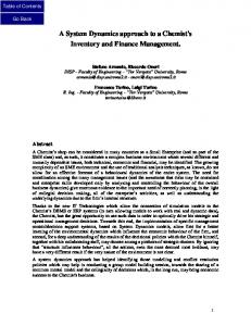
feedback loops that then are used in the modelling part, (ii) model conceptualization/model building: A sign causal diagram helps to understand the influences between the variables/elements. Model building uses explicit concepts of system dynamics that are transforming the flows into levels, rates and auxiliary variables, and (iii) running the simulation model/using the results: Once the model is built, different scenarios are analyzed and used to test different policies/decisions. The above three steps are applied to the current inventory system and are described as follows. At the airport fuel station, the inventory manager places an order to the refinery to refill the airport tanks to the maximum capacity on a daily basis. The main idea is that the demand rate reduces the inventory level and creates a gap below maximum tank capacity level. To fill this capacity gap, fuel order is placed to fill again the tank capacity to maximum level. The complete current inventory management model is built using Power-sim software and is shown in Fig. 1. Table 1 summarizes the equations that relate all the interrelations among the events of the current inventory management system. The output of this model calculates the total inventory cost; which is the sum of the holding, shipping, and material costs. Given that the DOH is always fixed to one day, the inventory model is evaluated by simulation for one year at three price level scenarios, including high, middle, and low of $ 800, $ 900, and $ 1000 per ton, respectively. The corresponding total inventory costs are found $32,417,653, $35,696,704, and $40,522,130, respectively.

expected demand is represented by a level, the “change in expected demand”, is “change in expected demand”= (“demand rate”“Expected demand”)/“time to change expectations”

III. THE PROPOSED MODEL FOR IMS

The "Supply orders" are linked with the “Supplies”, which is calculated as

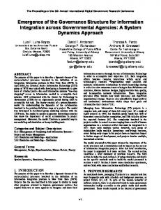
Following the same steps of system dynamics, the proposed model is constructed and is depicted in Fig. 2. In this figure, the model includes two key sides: demand and supplies. Fuel inventory is modeled as a “fuel level”, which increases or decreases depending on fuel supply or demand rate. The initial value equals 150 tons. Fuel supplies add to the “fuel level”, whereas fuel demand drains. Then, the available tank capacity equals tank capacity minus “fuel level”. The “Expected demand” is an important part of this model because it translates changes in demand “demand rate” into changes in refilling rate by supplier. It is used to shock the model to reveal its behavior. The “Expected demand” is forecast of fuel demand rate. The forecast function returns the forecasted value of demand rate by computing the first order exponential average of demand rate using an averaging of past, which equals five days, and then extrapolates the trend a distance equal to future time of one day. The “time to change expectations” is a constant which represents the time needed to adjust expectations about demand into real demand. Flows are the only elements that change levels. Since


The "Desired supplies" represents a desired accumulation and the real one. To achieve customer satisfaction, it is assumed that the “Desired supplies” should always reflect the “Expected demand”. Then, the “Desired supplies” is expressed as “Desired supplies” = “Expected demand” + (“Desired fuel level”–“fuel level”)/lead time where, the “Desired fuel level” is initially assumed to cover 3 days, and “Desired fuel level”= “Expected demand” ” fuel coverage” where, the “fuel coverage” represents the desired number of day's sales that should be covered by the fuel in tanks. In this research, it is considered the decision variable in the optimization model. Its initial value equals one. The lead time is a constant which equals eight hours. The “Supplier orders” are determined based on the “Desired fuel level” and the “available capacity of the tanks”. In this model, it takes the value of the minimum amount between “available capacity” and “Desired fuel level-fuel level”. That is, “Supplier orders” = Minimum {available tank capacity, (“Desired fuel level”-“fuel level”)}

“Supplies”= Delaymtr(supply orders, lead time)/time step where, the Delaymtr function returns the nth order exponential material delay of “Supply orders” using an exponential averaging time delay. The material delay resulted from the delay for processing of fuel. The lower part of the model represents the total inventory cost, which composed of holding cost, shipping/carrying cost, and fuel cost. Holding cost is calculated as Holding cost = holding cost factor  suppliesprice where, holding cots factor is a constant of 0.3. Supplies cost is the cost of the fuel carried in inventory multiplied by fuel price. Shipping cost is expressed as Shipping cost = number of trucks  cost per truck Finally, supplies cost is estimated as

WCE 2010


Supplies cost = Price  Supplies The sum of the above three costs gives the total inventory cost. Table 2 summarizes the related equations of the proposed model. The model starts by producing a random “Demand rate” based on various time-based demand functions, through a delay, to evaluate the expected future demand and consequently determine “fuel coverage” that minimizes total inventory cost, while avoiding stock out. A. Assumptions, Parameters, and Constraints In building the simulation model for the fuel inventory system under study, the following assumptions are made: (1) the demand is exponential over a year, (2) once an order is placed, it cannot be modified, (3) the capacity of the supplier (refinery) is infinite, (4) all orders are delivered by trucks at same day, and (5) the company knows the current fuel inventory level at any instant of time. The parameters are determined based on manager’s knowledge: (i) the company has only one fuel supplier, (ii) fuel tank capacity is 300 tons, (iii) the cost of shipping is $40, (iv) fuel prices are deterministic, thus different fuel price values are used as inputs, (v) truck capacity is 40 tons, and (vi) lead time is eight hours calculated from the hour the order is placed to that the fuel tank arrives. The model should consider that for each time horizon of the model, the supplies should not exceed the upper limit of full tank capacity, stock out is not allowed, and thus 100 % customer satisfaction is achieved in all time periods, and the company can receive up to 300 ton per day. Finally, the main objective is to determine the optimal DOH that reduces the total inventory costs while avoiding stock out. B. Optimization of total inventory costs An evolutionary search method is adopted to generate new values for the decision sets using computer software. On the basis of the value intervals and constraints defined for our decisions, new parameters are generated and used in the simulation. Those that produce the best results are used as parent values to generate new offspring values. This process is repeated until the goal is reached, or the convergence rate is too low. In order to be able to add different scenarios for demand rate shown in Fig. 3, three step-functions are used. The high, middle, and low demand rate functions are 60+step (30), 30+step (20), and 1+step (30) with durations 0.5, 1.5, and 10 months, respectively. System dynamics simulations are performed for three price levels. This results for nine price and demand level optimization scenarios are shown in Table 3. The optimal DOH and total inventory cost are tabulated in Table 4 for all nine level combinations. The total inventory cost at each price level is then calculated as the sum of inventory costs


for all the three demand rate functions at each price level. The estimated total inventory costs at low, middle, and high price levels are found $2238680, $2514500, and $2790920, respectively. C. Comparison of total inventory costs Compared to current inventory policy, the proposed inventory ordering policy resulted in tremendous savings, which are calculated as the difference of the total inventory cost between the current and proposed models, by $30,178,973, $33,182,204, and $ 37,731,210 for low, middle, and high price levels, respectively. A major contribution to these savings is that the optimal DOH at low demand of 10 months duration is more than three days for the three price levels, in contrast with the inventory ordering policy of one day at current situation. IV. RISK ASSESSMENT The risk assessment analysis performs the sensitivity analysis by finding set of samples for the assumptions and then running a simulation run for each of these samples. Two sampling methods Monte Carlo and Latin Hypercube are often used. The Latin Hypercube method is ten times as efficient as the Monte Carlo method and hence it will be used in the risk assessment of total inventory cost. In this research, the Latin Hypercube method with 300 generations and seed of 100 is employed to investigate how sensitive proposed model to the assumption made and identify which assumptions have the highest influence on the model. The decision is the fuel coverage, whereas the assumptions are the lead time, holding cost factor, information delay. Finally, the total inventory cost is the effect. A. Random lead time The lead time is assumed normally distributed with mean and standard deviation of 0.3 and 0.3 day, respectively. Initially, the sensitivity analysis is conducted at low levels order rate and demand with the corresponding optimal DOH of 3.551 days. The 10 % to 90 % percentiles of total inventory cost at low price and demand levels are displayed in Fig. 3(a). Obviously, the total inventory cost is insensitive to variations in the lead time of the above distribution, because the difference between the 10 % and 90 % percentiles are almost the same. B. Random information delay The optimal DOH was obtained at fixed value of information delay of 3 days. The information 4delay represents the time it takes for demand information to reach management. In this part, the information delay is assumed normally distributed with a mean and standard deviation values of 3 and 1 days, respectively. Fig. 3(b) displays the sensitivity analysis at low levels order rate and demand. It is noticed that

WCE 2010


the differences between the 10 % and 90 % percentiles are negligible. Hence, the total inventory cost is concluded insensitive to varying the information delay. C. Random holding cost factor Initially, the model was evaluated with a cost factor of 3 %. To investigate the effect of varying the holding cost factor on total inventory cost, this factor is varied cost uniformly distributed with minimum and maximum values of 2 % and 4 %, respectively. Fig. 3(c) depicts the obtained results of sensitivity analysis with varied holding cost factor at low price and demand levels combination. Clearly, the total inventory cost is found insensitive to change in the cost factor, because of the negligible differences between 90 % and 10 % percentiles. The sensitivity analysis is conducted for the other eight combinations of price and order rate in a similar manner. Interestingly, the optimal DOH values obtained earlier are insensitive to varying the lead time, information delay, and holding cost factor.

V. CONCLUSIONS

An airline fueling system aims at maintaining fuel inventory level at proper levels to avoid stock out, without building excessive inventory levels. This research built an optimization model based on the ideas of systems thinking and system dynamics to achieve this goal considering exponentially distributed fuel demand. The effectiveness of fuel inventory system is measured by fuel coverage, which is treated as a decision variable in the optimization model. The optimization results for DOH resulted in huge savings in total inventory cost and are found insensitive to variations in lead time, information delay and time to change expectations. Definitely, the DOH values obtained in this research shall provide great assistance in deciding fuel inventory level and ordering quantities at planning stage.


REFERENCES [1]

A.P. Morris, J. Sandling, R. Fancher, M. Kohn, H-P. Chao, and W. Chapel, “A utility fuel inventory model,” Operations Research, 1987, 35(2), 169-184. [2] S. Bonser, and D. Wu, “Procurement planning to maintain both short-term adaptiveness and long-term perspective,” Management Science, 2001, 47(6), 769–786. [3] K. Abdelghany, A. Abdelghany, and S. Raina, “A model for the airlines’ fuel management strategies,” Journal of Air Transport Management, 2005, 11, 199–206. [4] J. Basso, and A. Zhang, “On the relationship between airport pricing models,” Transportation Research Part B, 2008, 42, 725–735. [5] J. Forrester, Industrial Dynamics. MIT press, Cambridge, MA, 1961. [6] J.D. Sterman, Business Dynamics: Systems Thinking and Modeling for a Complex World. McGraw-Hill Higher Education, New York, 2000. [7] L. Alfeld, and A. Graham, Introduction to Urban Dynamics. Cambridge, MA: The MIT Press, 1976. [8] N.A. Repenning, “A simulation-based approach to understanding the dynamics of innovation implementation,” Organization Science, 2002, 13, 109–127. [9] J. Homer, G. Hirsch, M. Minniti, and M. Pierson, “Models for collaboration: How system dynamics helped a community organize cost-effective care for chronic illness,” System Dynamics Review, 2004, 20, 199–222. [10] P. Hjorth, and A. Bagheri, “Navigating towards sustainable development: A system dynamics approach,” Futures, 2006, 38, 74–92. [11] J.W. Stevenson, Operations Management. MCGraw-Hill: Irwin, 2005. [12] R.U. Ricardo, and P.C. Alberto, “Soft System Dynamics Methodology (SSDM): Combining Soft Systems Methodology (SSM) and System Dynamics (SD) ,” Systemic Practice and Action Research, 2005, 18(3); 303-334.

WCE 2010


Table 1. The equations of the systems thinking model for the current situation. Name

Definition.

Unit.

Fuel level.

Initial value=150

Ton

Supplies

Delaymtr(Shipping amount, delivery delay)

Ton/day

Airplanes fueling

Fuel demand Exprnd (1.56*E^4)

Ton/day

Delivery delay

0.3

day

Desired fuel level

300

Ton

Shipping amount Truck capacity

IF ('fuel level'