also occurs in lm from high speed cameras used to record the evolution of short duration ..... The detection and correction of artefacts in archived gramophone.
A system for reconstruction of missing data in image sequences using sampled 3D AR models and MRF motion priors Anil C. Kokaram and Simon J. Godsill Signal Processing and Communications Group, Cambridge University Engineering Dept., Cambridge CB2 1PZ, England
Abstract. This paper presents a new technique for interpolating missing data in image sequences. A 3D autoregressive (AR) model is employed and a sampling based interpolator is developed in which reconstructed data is generated as a typical realization from the underlying AR process. In this way a perceptually improved result is achieved. A hierarchical gradient-based motion estimator, robust in regions of corrupted data, employing a Markov random eld (MRF) motion prior is also presented for the estimation of motion before interpolation.
1 Introduction The problem of missing data reconstruction in image sequences has traditionally not been fully addressed by the computer vision and video processing communities in the past. Various order statistic operations have been proposed for the suppression of impulsive noise in image sequences [1] but in general the problem of reconstructing missing data has been seen as a subset of the impulsive noise problem. An important example of missing data degradation is found in the motion picture industry. Particles caught in the lm transport mechanism can damage the image information. The missing data regions manifest themselves as `blotches' of random intensity in the sequence, known as `Dirt and Sparkle'. The problem also occurs in lm from high speed cameras used to record the evolution of short duration events such as explosions or impacts. In all these cases, the image information in the corrupted area is largely destroyed. This work considers the development of spatio-temporal processes for detection/interpolation. The detection/estimation approach is adopted here in order to treat only suspected areas of distortion. This is an alternative philosophy to the usual global application of median lters employed to solve this problem. In addition, for good detail preservation of texture, it is necessary to look beyond the use of median lters to a model based approach for texture generation. The paper is organized as follows: section 2 describes the new robust motion estimation/correction methods and also brie y describes the blotch detection scheme (See [2]); section 3 describes the 3D AR model and robust parameter estimation for that model; section 4 describes the sampling based interpolation scheme; section 5 presents results obtained from processing degraded lm image sequences; and nally section 6 concludes the paper and discusses future directions for the work.
2 Motion estimation and the detection of blotches Corrupted pixels, which are part of `blotches' in the image sequence, generally do not occur in the same spatial location and with the same brightness in consecutive frames. They are therefore well de ned as temporal discontinuities in the image sequence. Blotches can be distinguished from sites of occlusion and uncovering because they are at sites which are `occluded' in both the next and previous frames (i.e. this image information does not exist in either of the two surrounding frames). Sites of occlusion and uncovering, however, represent discontinuities in either the backward or forward temporal direction, but never both. A simple but e�ective detector (SDIa) for corrupted pixels was presented in [2]. It ags
pixels as corrupted, when both the squared motion compensated pixel di�erences (forward and backward in time) are larger than some user de ned threshold. The reader is encouraged to refer to [2] for details. Robust motion estimation is important for the correct operation of the detector. The next section presents a new technique for gradient based motion estimation, using a combination of low-level video processing algorithms.
2.1 Multiresolution Wiener Based Motion Estimation
There exist many formulations for pel-recursive, translational, motion estimators which successively re ne an estimate for the displacement between frames n and n ? 1 at location ~x, d~n;n?1(~x). This is achieved via updates calculated through a Taylor series expansion of the image function around the current estimated displacement. These appear to have been somewhat overlooked by the computer vision community. Biemond [3] presented a Wiener solution for an update displacement, ~u^ i , which is more robust to noise. Errors in this motion estimator can be linked directly to the extent of ill{conditioning in a gradient matrix, Mg = [GT G] (see below). At an edge in the image, it is clear that the motion estimate is most con dent in the perpendicular direction. Yet it is at just such locations that Mg can be ill-conditioned. This fact was recognized independently by Martinez, [4], who employed the SVD of Mg in an earlier work on a non-iterative gradient based motion estimation scheme. In the case where the estimator was at an edge, it was possible to salvage some useful information by aligning the extracted motion vector with the direction of maximum image gradient, using the SVD. This paper therefore proposes a combined strategy for an adaptive Wiener based (AWB) motion estimation scheme in which the update displacement, ~ui , is generated as follows,
8 < �max~kmax if ��max min > � h i ~ui = : T ?1 T G G + �I G z otherwise � = jzj ��max if ��max min � �
(1)
min
�max
~T = �kmax GT z max
where �; ~k refer to the eigenvalues and eigenvectors of GT G, and �max is a scalar variable introduced to simplify the nal expression. In this combined strategy, the condition of Mg is monitored through �. When the condition number ( ��max min ) is larger than this value, the SVD of Mg is used to generate the `valid' motion component. Otherwise, Mg is assumed to be well conditioned and the regularized wiener solution for the update is used in which � is proportional to the product of the magnitude of the current DFD and the condition of the matrix[5].
2.1.1 Implementation
The AWB estimator is incorporated into a block based scheme where each block in the image is assigned one motion vector. In order to reduce computation and the occurrence of spurious vectors, the AWB estimator is only employed in blocks where motion is detected. This consists of thresholding the mean absolute error (MAE) between the current block and the block at the same location in the previous and next frame. An MAE larger than the threshold is assumed to indicate motion and only in that case is motion estimation engaged. Gradient based motion estimation schemes only work when the Taylor series expansion of the image function is valid i.e. when estimating small displacements. In most interesting image sequences, especially those in movies, the assumption of small motion is not valid. This can be overcome through a multiresolution strategy for motion estimation in a similar way to [6, 7]. For the implementation in this paper, an L level image pyramid (2:1 subsampling) is generated using an FIR gaussian kernel with variance 1.5 and window size 9 � 9. After n iterations of the AWB motion estimator, the vectors are propagated down to
the next level and used as initial estimates for motion estimation at that level. At the original resolution level, it is typical that some areas which are not moving are assigned motion vectors only because of their proximity to moving regions in the upper levels of the pyramid. This motion halo e�ect is reduced in the manner of [8] by double checking for motion at level 0 in the pyramid.
2.2 Vector eld correction
After motion estimation is complete, the SDIa detector can be used to ag pixels which are detected as corrupted. These pixels can be grouped together as necessary to measure the spatial extent of each blotch. The problem now is to ll the indicated region with some realistic estimate for the missing image data. This requires using information from both the next and previous frames. But the motion estimates are detrimentally a�ected by the presence of a Blotch. Therefore, an interpolated vector is required at this site. Also important is to ensure that the interpolation process is robust enough to ignore or to de-emphasize data collected using an incorrect motion vector. This is discussed in the next section. It is assumed that motion vectors in frame n constitute a Markov Random Field (MRF)1 . The conditional probability of the vector d~n;n?1 (~x) given the frames In and In?1 and some neighborhood subset of motion vectors, Sn (~x), can be written using Bayes theorem as
~ ~ p(d~n;n?1 (~x)jIn ; In?1 ; Sn (~x)) = p(In; In?1 jdn;n?p1(I(~x;);ISn (j~xS))p(~x(d))n;n?1 (~x)jSn (~x)) n n?1 n
(2)
The situation between frames n; n + 1 can be written similarly. The likelihood is taken as a zero mean gaussian distribution of DFD's, with variance �e2 . Note that the vector eld considered is de ned on the block lattice and not the pixel lattice. Therefore the likelihood should contain a contribution from every pixel in the block centered on location ~x as follows (dropping Sn (~x) for brevity),
0 1 X p(Ijd~n;n?1(~x)) / exp ? @ 1 2 w2 (~x)[In (~x) ? In?1 (~x + d~n;n?1 (~x))]2 A 2�e ~x2B
(3)
where B is the set of all locations in the block and I represents In ; In?1 . A weight w(~x) is associated with each DFD measurement. This weight is set to 0 wherever the pixel site is agged as corrupted by the detector, and set to 1 otherwise. Nw is the sum of these weights over the block. In the manner of e.g. [11, 12] a Gibbs Energy prior is used for d~n;n?1 (~x) as follows
0 1 X p(d~n;n?1 (~x)jSn (~x)) / exp ? @ �(~v)[d~n;n?1 (~x) ? ~v]2 A ~v2Sn (~x)
(4)
where ~v is each vector in the neighborhood represented by Sn (~x), and �(~v ) is the weight associated with each clique. The situation is illustrated in the left hand portion of gure 1. Note that the cliques employed here assume rst order interactions even though the eight connected neighborhood can involve some second order cliques [9]. In order to discourage `smoothness' over too large a range, �(~v ) is de ned as �(~v ) = Nw =jX~ (~v) ? ~xj where X~ (~v ) is the location of the block providing the neighborhood vector ~v. This location is measured in terms of block lengths. As before, Nw is the number of uncorrupted pixels in the block. Large �(~v ) encourages motion vector smoothness, and small �e2 encourages vectors which minimize the DFD. It is true that equations 2, 3, 4 are su�cient to estimate the motion eld itself [9, 11], and the prior can be altered to account for motion discontinuities. However, a direct solution for the MAP estimate (2) with respect to the vector eld (via some Monte Carlo technique) is computationally demanding [9]. In practice, after the use of the AWM estimator and the blotch detector, it is already possible to make a very con dent assessment of the locations of corruption. Therefore, there is no longer interest in 1 It is assumed that the reader is familiar with the concept of Markov Random Fields.
See [9, 10, 11].
Block Based Vector
Data block of N points
Clique Interactions
Blotch
Figure 1: Left : Neighborhood and cliques used for p(dn;n?1 (~x)). Right : Altered Neighborhood used with a large blotch. the uncorrupted regions. Rather than relax the vector eld around the corrupted location using, e.g. the Gibbs Sampler [9], it is found su�cient to reduce the solution search space2 to the vectors in the neighborhood of the blotch. Each vector in turn is tested as a candidate solution to the corrected vector by substitution in equation 2. The candidate which maximizes 2 is selected as a working approximation to the MAP estimate. Note that the denominator of equation 2 is constant and can be ignored. An estimate for �e2 is made from the measured DFD for each vector candidate. In the case where the DFD does not vary much with di�erent candidate vectors, the operation reduces to a type of weighted vector median. When the blotch engulfs several blocks, the candidate vector set is chosen from an altered neighborhood where the blocks concerned contain less than 10% corruption. This strategy is illustrated in gure 1.
3 The 3D AR Model The structure of the AR model allows e�cient computational algorithms to be developed, and it is this, together with its spatiotemporal nature which is of interest. The physical basis for its use as an image model for interpolation is limited to its ability to describe local image smoothness both in time and space. The 3D AR model model equation is as follows.
I (~x; n) =
P X k=1
ak I (x + qxk + dxn;n+qnk (~x); y + qyk + dyn;n+qnk (~x; n + qnk )) + �(~x; n)
(5)
In this expression, I (~x; n) represents the pixel intensity at the location ~x = (x; y) in the nth frame. There are P model coe�cients ak , and the spatiotemporal model support is de ned by the vectors ~qk = [qxk ; qyk ; qnk ]. The support locations are o�set by the relative displacement between the predicted pixel location and the support location. The displacement between frame n and frame m is d~n;m (x; y) = [dxn;m (x; y); dyn;m(x; y)]. Finally, �(x; y; n) is the prediction error at location (x; y; n). Figure 2 shows a temporally causal 3D AR model with 5 pixels support. In this paper the parameters of the model are estimated using weighted least squares [2]. The weights assigned to each prediction equation are 0 where the blotch detector has agged a corrupted pixel site and 1 otherwise. �(x; y; n) is assumed to be drawn from a white Gaussian noise process with variance ��2 . 2 A similar simpli cation was made by Stiller [12] for motion eld smoothing.
No displacement
Displacement of [-1 -1]
Motion vector
Motion vector Frame n-1
Frame n-1
Frame n
Frame n Support pel Predicted Pel
Figure 2: Handling motion with the 3D AR model.
4 Interpolation Given the position of missing pixels, motion estimates and AR parameters for a sub-block of the image, the missing information is now interpolated. The methods currently proposed [2] reconstruct the missing data with an interpolation which minimizes the excitation energy in a least-squares sense. However, this solution, which is equivalent to the maximum a posteriori (MAP) estimate under Gaussian assumptions [13], tends to be oversmooth compared with surrounding pixels, especially when the missing area is large. The problem is well illustrated in gures 3, 6. Oversmoothing in the reconstructed image occurs because estimation techniques which use these or other familiar objective functions do not make allowance for the random component in image sequences, which cannot be predicted exactly from surrounding pixel values. We propose an interpolator which draws the missing pixel values as a random sample from their posterior probability distribution conditional upon the known pixel values which surround the missing region. In this way the interpolation will be typical of the AR process under consideration and should not exhibit the oversmooth nature of other interpolators. Similar principles have been successfully applied to the interpolation of missing samples from audio signals which can be modelled as a 1-d AR process [14, 15, 16].
4.1 Sampled interpolations The vector of excitation values e corresponding to a block of data i is written in matrix-vector notation as e = Ai, where A is constructed from the AR parameter vector a in such a way as to generate �(!r ) !
(see (5)) for N distinct values of r . This expression can be partitioned into a part corresponding to known data pixels iK and unknown data iU , leading to Ai = AK iK + AU iU , where AK and AU are the corresponding columnwise partitions of A. Under Gaussian and independence assumptions for the excitation process the posterior distribution for the missing pixels is given by (see appendix A)
�
U AU j exp ? 1 (i ? iMAP )T (AT A ) (i ? iMAP ) p(iU jiK; �e2 ; a) = jA U U U U 2�e2 U U (2��e2 )l=2
T
1=2
�
(6)
which we note is in the form of a multivariate normal distribution. iMAP is the standard MAP/least U squares (see [13, 2]) interpolator, given by: T ?1 T iMAP U = ?(AU AU ) AU AK iK
(7)
An estimate for �e2 in equation (6) can be made from observations of the excitation in the uncorrupted region around the missing pixels following AR parameter estimation.
Figure 3: Degraded Frame 2 of FRANK with large blotches boxed.
Figure 4: Detected Blotches (bright white) in Frame 2, after dilation of detection eld.
Drawing a random sample from the multivariate normal distribution of equation (6) can be achieved using well known procedures and may be summarized as:
ui � N(0; 1); (i = 1 : : : l)
?1 isamp = iMAP U U +S u
(8) (9)
where `�' denotes a random draw from the distribution to the right, N(0; 1) is the standard normal distribution and S is any convenient (l � l) matrix square-root factorization which satis es ATU AU =�e2 = ST S. u is the column vector formed from the elements ui. The sampled interpolation isamp can then be U substituted for the missing pixels in the restored image. Drawing a sample from the conditional distribution can be seen to involve calculation of the MAP ?1 ?1 estimate iMAP U and adding an appropriately coloured noise term S u. Calculation of S need not involve any signi cant overhead over MAP interpolation if a matrix square-root factorization method such as Cholesky Decomposition is used in the inversion of ATU AU (equation (7)).
5 Results Because the sampling based interpolator draws a typical sample for the interpolated data, it is not possible to measure the performance of the interpolator by using a standard distortion measure such as MSE with arti cially degraded sequences, since the MAP estimate is likely to give the give the lowest MSE. Indeed that is its shortcoming. Therefore it is best to illustrate performance by using visual comparisons. Figure 3 shows a frame of a real degraded sequence. The overall motion in the sequence is a rapid vertical pan, with some fast motion in the petals of the ower and some complicated motion in the background trees. The blotches to be considered are highlighted in gure 3. Each frame is of resolution 256 � 256. A 2 level pyramid was employed for motion estimation. The block size used was 9 � 9, the motion threshold was 10:0 grey levels, 10 iterations of the AWB estimator were used at each level, and � = 100:0. The blotch detection threshold, et was set at 25:0. The areas which were then agged as corrupted (using SDIa , see [2]) are shown as bright white pixels in gure 4, superimposed on a darkened version of frame 2 ( gure 3). Note the false alarms in the region of the petals of the ower - the petals themselves are quite impulsive features which do not move smoothly from frame to frame. The block based motion estimation technique does not function well here. Figures 6 and 5 show a zoomed version of the MAP reconstruction with and without vector eld correction respectively. The interpolated regions are boxed in white. The improvement is illustrated
Figure 5: Interpolation using MAP estimate without vector correction. (Interpolated regions boxed.)
Figure 6: Interpolation using MAP estimate with vector correction. (Interpolated regions boxed.)
Figure 7: Interpolation with spatiotemporal median lter. (Interpolated regions boxed.)
Figure 8: Sampled Interpolation. (Interpolated regions boxed.)
clearly in the large blotch (shown on frame 2). The interpolated data is much better in keeping with the rest of the hairstyle when the motion vector used at the blotch site has been `corrected'. The 3D AR model used here was causal with support only in the previous frame in a 3 � 3 block of 9 support points. The improvement in quality with motion eld correction is the same whatever the interpolation employed and so no more examples are given. Figures 7 and 8 show a zoomed version of the results of a controlled median ltered operation and a sampled AR interpolation (section 4) respectively. The interpolated regions are also boxed in white. The ML3Dex lter as de ned in [2] was used at the sites of detected distortion to generate gure 7. The same 3D AR model as for the MAP interpolation of gure 6 was used. Both results employed the corrected vector eld in assembling the motion compensated data for interpolation. The median ltered result is the worst of the 3 alternatives ( gures 6, 8, 7) as it cannot reconstruct the texture properly across the large blotch in particular. To be fair, however, the median ltering strategy does not ignore pixels from its mask which are known to be corrupted; if this were done the median result could be better. In the regions which are not heavily textured, e.g. the background blotches, the median result compares well with the model based interpolations. The sampled AR process ( gure 8) has reconstructed the missing data including the detail extremely well. Where the MAP interpolation has introduced a slight smoothing e�ect, the sampled interpolator has recreated the random `graininess' which is typical of the surrounding area in the image. This is seen best if the interpolated regions in the large blotch are compared in gures 6 and 8. Furthermore, note that even though it is clear that the `corrected' motion vector used at the blotched location is not necessarily 100% accurate3 , this has not detrimentally a�ected the model based interpolation schemes. In fact, because of the spatial extent of the model support in the previous frame, the model can cope, in this case, with inaccuracies of up to �1 pixel in the motion vector used.
6 Conclusions and Further Work This work has presented a new scheme for detail preserving interpolation of missing data in image sequences. In achieving this goal, it has also introduced a new technique for gradient based motion estimation. It has also been pointed out that when the vector eld model is based on an MRF prior employing a Gibbs Energy distribution, an initial con guration that is close to the nal true solution will of course improve the convergence of the relaxation algorithms [9]. Such initial estimates can be had using any number of lower complexity motion estimation algorithms [3, 7] which do not explicitly allow for motion discontinuities, for instance. A new sampling based interpolator has been introduced which does not su�er from the `oversmoothing' of large missing regions and which does not substantially increase the computation required. Finally, it must be noted that in achieving the goal of missing data interpolation, this paper has employed 3 di�erent models of the image sequence in order to address conveniently each sub-problem as it arises. Translational motion is a convenient model for generating a fast initial con guration for the motion eld. Equation 2 is a probabilistic formulation which then allows the correction of the vector eld through an image sequence model which imposes an implicit constraint on the smoothness of the motion eld. The AR model equation 5 then imposes some constraint on the image values to allow the interpolation of the missing region. All of these formulations emphasize a di�erent aspect of the image sequence and it is possible to combine them all into a single Bayesian framework for the estimation of the various parameters, including the missing data itself. This is the current focus of our research.
A Posterior probability for interpolated data We derive here the conditional posterior probability expression for the missing pixels, given in equation (6). 3 Essentially, it has been estimated by replacing it with one of the surrounding vectors.
Assuming a Gaussian independent excitation with variance �e2 we can write down the probability for e as T e! e 2 ? N= 2 p(e) = (2��e ) exp ? 2�2 e
The distribution for the corresponding block of image pixels i is then obtained by the change of variables e = Ai (see section 4.1), giving: T T Ai p(i) = p(e = Ai) = (2��e2 )?N=2 exp ? i A 2�2 e
!
(10)
Note that this distribution is strictly conditional upon a minimal region of AR support pixels at the edges of the block (see e.g. [17] for the 1-d case), but we omit this dependence here for clarity of exposition. The form of the nal result for missing pixels is unchanged by this simpli cation provided the region of support contains only known pixels. The above expression also assumes a causal AR model (in which case the Jacobian for the variable change is always unity). The conditional distribution for missing pixels iU is then obtained from the probability chain rule as: p(iU jiK) = pp((ii)) K Note that the denominator term in this expression is constant for any given image and AR model. Hence the nal result can be determined by rearrangement of (10) in terms of iU and noting that the resulting distribution must be normalized w.r.t. iU . Substituting Ai = AK iK + AU iU (see section 4.1) into equation (10) and rearranging to give a normalized distribution leads to the nal result of equation (6).
References [1] G.R. Arce. Multistage order statistic lters for image sequence processing. IEEE Transactions on Signal Processing, 39:1146{1161, May 1991. [2] A. Kokaram, R. Morris, W. Fitzgerald, and P. Rayner. Detection/interpolation of missing data in image sequences.. IEEE Image Processing, pages 1496{1519, Nov. 1995. [3] J. Biemond, L. Looijenga, D. E. Boekee, and R.H.J.M. Plompen. A pel{recursive wiener based displacement estimation algorithm. Signal Processing, 13:399{412, 1987. [4] D. M. Martinez. Model{based motion estimation and its application to restoration and interpolation of motion pictures. PhD thesis, Massachusetts Institute of Technology, 1986. [5] L. Boroczky J. Driessen and J. Biemond. Pel{recursive motion eld estimation from image sequences. Visual Communication and Image Representation, 2:259{280, 1991. [6] W. Enkelmann. Investigations of multigrid algorithms for the estimation of optical ow elds in image sequences. Computer Vision graphics and Image Processing, 43:150{177, 1988. [7] J. Kearney, W.B. Thompson, and D. L. Boley. Optical ow estimation: An error analysis of gradient based methods with local optimisation. IEEE PAMI, pages 229{243, March 1987. [8] M. Bierling. Displacement estimation by heirarchical block matching. In SPIE VCIP, pages 942{951, 1988. [9] R. D. Morris. Image Sequence Restoration using Gibbs Distributions. PhD thesis, Cambridge University, England, 1995. [10] S. Geman and D. Geman. Stochastic relaxation, gibbs distributions and the bayesian restoration of images. IEEE PAMI, 6:721{741, 1984. [11] J. Konrad and E. Dubois. Bayesian estimation of motion vector elds. IEEE Trans PAMI, 14(9), September 1992.
[12] C. Stiller. Motion{estimation for coding of moving video at 8kbit/sec with gibbs modeled vector eld smoothing. In SPIE VCIP., volume 1360, pages 468{476, 1990. [13] R. Veldhuis. Restoration of Lost Samples in Digital Signals. Prentice-Hall., 1990. [14] P. J. W. Rayner and S. J. Godsill. The detection and correction of artefacts in archived gramophone recordings. In Proc. IEEE Workshop on Audio and Acoustics., 1991. [15] J. J. K. O� Ruanaidh and W. J. Fitzgerald. Interpolation of missing samples for audio restoration.. Electronic Letters., 30(8), April 1994. [16] J. J. Rajan, P. J. W. Rayner, and S. J. Godsill. A Bayesian approach to parameter estimation and interpolation of time-varying autoregressive processes using the Gibbs sampler. Submitted to IEEE Trans. on Signal Processing., June 1995. [17] M. B. Priestley. Spectral Analysis and Time Series. Academic Press, 1981.