A taxonomy for the virtual machine allocation problem

A taxonomy for the virtual machine allocation problem∗ Zoltán Ádám Mann† Department of Computer Science and Information Theory Budapest University of Technology and Economics Budapest, Hungary

Abstract Recently, the virtual machine allocation problem, in which virtual machines must be allocated to physical machines in cloud data centers, has received a lot of attention. This is a very complex optimization problem with many possible formulations. In order to foster the clear definition of problem variants and the comparability of algorithms to solve those problem formulations, this paper introduces a generic model of the problem and derives the typically investigated problem variants as special cases. Meaningful problem variants are structured in the form of a taxonomy of problem models.

Keywords: Cloud computing, Problem formalization, Problem modeling, Virtual machines, VM placement

1

Introduction

Resource management in data centers (DCs) has been an important optimization problem for decades [7]. More recently, the wide spread of virtualization technologies and the cloud computing paradigm have established several new possibilities for resource provisioning and workload allocation [4], opening up new optimization opportunities but at the same time also introducing new challenges. Virtualization makes it possible to co-locate multiple applications on the same physical machine (PM) in logically isolated virtual machines (VMs). This way, a high utilization of the available physical resources can be achieved, thus amortizing the capital and operational expenditures associated with the purchase, operation, and maintenance of the DC resources (PMs, cooling, etc.). What is more, live migration of VMs makes it possible to move a VM from one PM to another one without noticeable service interruption [2, 14]. This enables the dynamic re-optimization of the allocation of VMs to PMs, reacting to changes in the VMs’ workload and the PMs’ availability. Consolidating multiple VMs on relatively few PMs helps not only to achieve good utilization of hardware resources, but also to save energy because unused PMs can be switched off or at least to a low-energy state such as sleep mode. However, too aggressive consolidation may lead to performance degradation. In particular, if the load of some VMs starts to grow, this may result in an overload of the accommodating PM’s resources, leading to a situation where one or more VMs will not receive the capacity that would be necessary to achieve acceptable performance. In many cases, the expected performance levels are laid down in a service level agreement (SLA), defining also penalties if the provider fails to comply. Thus, the provider must find the right balance between the conflicting goals of utilization, energy efficiency, and performance [13, 17]. Beside virtualization and live migration, the most important characteristic of the cloud computing paradigm is the availability of online services with practically unbounded capacity that can be provisioned elastically as needed. This includes Software-as-a-Service, Platform-as-a-Service, and Infrastructure-as-a-Service [34]. In the latter case, VMs are directly offered to customers; in the first two cases, VMs can be used to provision virtualized resources for the software/platform services in a flexible manner. Given the multitude of available public cloud offerings with different capabilities and pricing schemes, it is increasingly difficult for customers to make the best selection for their needs. The problem is further complicated by hybrid cloud setups that are increasingly popular in enterprises [5]. In this case, VMs can be either placed on PMs in the own DC(s) or using offerings from external providers, thus further enlarging the search space. ∗ This paper was published in International Journal of Mathematical Models and Methods in Applied Sciences, volume 9, pages 269-276, 2015 † This work was partially supported by the Hungarian Scientific Research Fund (Grant Nr. OTKA 108947).

1

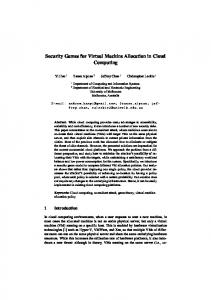
Real-world problem

Formalized problem model

Algorithm

Figure 1: General problem-solving process

Cloud Provider (CP)

Data Center (DC)

External Cloud Provider (eCP)

Data Center (DC) VM

PM

PM

PM

PM

PM

PM

PM

PM

VM VM VM

VM VM

VM VM VM

VM VM

VM VM VM

VM VM

VM VM VM

VM VM

VM VM

External Cloud Provider (eCP) VM

VM

VM

VM

Legend:

PM: Physical Machine

VM: Virtual Machine

Figure 2: Diagrammatic overview of the problem model There are several further aspects that need to be taken into account in VM allocation. For example, communication among VMs and network characteristics like bandwidth and latency of network elements lead to communication costs and delays that may be significant. Also live migration has an overhead in terms of both network communication and additional load on the affected PMs [30]. Another aspect is thermal management: if, for example, several PMs that are physically near to each other work under high load, this may lead to overheating, increasing the risk of failures [27]. Since the allocation of VMs is an important and challenging optimization problem, several algorithms have been proposed for it. However, as shown in a recent survey, the existing literature includes a multitude of different problem formulations – in fact, it is difficult to find a pair of papers in the VM allocation literature that address the same problem variant – making the existing approaches hardly comparable [19]. Even worse, some existing works failed to explicitly and precisely define the version of the problem that they are addressing, so that this must be figured out from the algorithm that they proposed or from the way the algorithm was evaluated. We believe that addressing an algorithmic problem should start with problem modeling: a thorough consideration of the problem’s characteristics and their importance or non-importance, leading to one or more precisely defined – preferably formalized – problem formulation(s) that capture the important characteristics of the problem [18]. Then and only then should algorithms be proposed if the problem is already well-understood and well-defined (see Fig. 1). It seems that in the case of the VM allocation problem, this critically important phase was skipped, resulting in a rather chaotic situation where algorithms for “the VM allocation problem” actually address many different problems with sometimes subtle, sometimes serious differences. The aim of this paper is to remedy this deficiency. Specifically, we devise and formally define a general formulation of the VM allocation problem that includes most of the problem formulations studied so far in the literature as special cases. We provide a taxonomy of important special cases and take a look at their complexity. Section 2 contains the general problem model and Section 3 discusses special cases, followed by a suggested notational system for VM allocation problem variants in Section 4. Finally, Section 5 concludes the paper.

2

General problem model

We consider a Cloud Provider (CP) that provides VMs for its customers. For provisioning, the CP can use either its own PMs or external cloud providers (eCPs); see Fig. 2 for a graphical overview. The CP attempts to find the right balance between the conflicting goals of cost-efficiency, energy-efficiency, and performance. In the following, we 2

describe the details of the problem.

2.1

Hosts

Let D denote the set of data centers available to the CP. For data center S d ∈ D, let Pd denote the set of PMs available in d, also including any switched-off PMs. Furthermore, P = {Pd : d ∈ D} is the set of all PMs. Each PM p ∈ P is characterized by the following numbers: • cores(p) ∈ N: number of processor cores • cpu_capacity(p) ∈ R+ : processing power per CPU core, e.g., in MIPS (million instructions per second) • capacity(p, r) ∈ R+ : capacity of resource type r ∈ R. For example, R can contain the resource types RAM and HDD, so that the capacity of these resources are given for each PM (e.g., in GB). This should be the net capacity available for VMs, not including the capacity reserved for the OS, the virtualization platform, and other system services Our approach to model the CPU explicitly and all other resources of a PM through the generic capacity function has several advantages. First, this gives maximum flexibility regarding the number of resource types that are taken into account. For instance, also caches, SSD drives, network interfaces, or GPUs can be considered, if relevant. On the other hand, the CPU is quite special, particularly because of multi-core technology. A multicore processor is not equivalent to a single-core processor of capacity cores(p) · cpu_capacity(p). It is also not appropriate to model each core as a separate resource, because VMs’ processing power demand is not specific to each core of the PM, but rather to the set of its cores as a whole. The other reason why it makes sense to model the CPU separately is the impact that the CPU load has on energy consumption. Each PM p ∈ P has a set of possible states, denoted by States(p). States(p) always contains the state On, in which the PM is capable of running VMs. In addition, States(p) may contain a finite number of low-power states (e.g., Of f and Sleep). Each PM p ∈ P and state ∈ States(p) is associated with a static power consumption of static_power(p, state) per time unit. In addition, the On state also incurs a dynamic power consumption depending on the PM’s load, as defined later. The possible state transitions are given in the form a directed graph (States(p), T ransitions(p)), where a transition ∈ T ransitions(p) is an arc from one state to another. For each transition ∈ T ransitions(p), delay(transition) and energy(transition) denote the time it takes to move from the source to the target state and the energy consumption associated with the transition, respectively. (It should be noted that most existing works do not model PM states and transitions in such detail; an exception is the work of Guenter et al. [12].) Let E denote the set of eCPs from which the CP can lease S VMs. For each eCP e ∈ E, T ypes(e) denotes the set of VM types that can be leased from e, and T ypes = {T ypes(e) : e ∈ E} is the set of VM types available from at least one eCP. Each VM type type ∈ T ypes is characterized by the same set of parameters as PMs: cores(type), cpu_capacity(type), and capacity(type, r) for all r ∈ R. In addition, for an eCP e ∈ E and a VM type type ∈ T ypes(e), f ee(type, e) specifies the fee per time unit for leasing one instance of the given VM type from this eCP. It should be noted that the same VM type may be available from multiple eCPs, potentially for different fees. Since VMs can be either hosted by a PM or mapped to a VM type of an eCP, let Hosts = P ∪ {(e, type) : e ∈ E, type ∈ T ypes(e)} denote the set of all possible hosts.

2.2

VMs

What we defined so far is mostly constant: although sometimes new PMs are installed or existing PMs are taken out of service, eCPs sometimes introduce new VM types or change rental fees, such changes are rare, and can be seen as special events. On the other hand, the load of VMs changes incessantly, sometimes quite quickly [33]. For the purpose of modeling such time-variant aspects, let T ime ⊆ R denote the set of investigated time instances. We make no restriction on T ime: it can be discrete or continuous, finite or infinite etc. The set of VMs in time instance t ∈ T ime is denoted by V (t). For each VM v ∈ V (t), cores(v) is the number of processor cores of v. The CPU load of v in time instance t is a cores(v)-dimensional vector: vcpu_load(v, t) ∈ cores(v) R+ , specifying the computational load per core, e.g., in MIPS. The load of the other resources is given by vload(v, r, t) ∈ R+ for a VM v ∈ V (t), resource type r ∈ R, and time instance t ∈ T ime. It should be noted that all the cores of a PM’s CPU are expected to have the same capacity. In contrast, the cores of the CPU of a VM do not have to have the same load. 3

2.3

Mapping VMs to hosts

The CP’s task is to maintain a mapping of the VMs to the available hosts. Formally, this is a function M ap : {(v, t) : t ∈ T ime, v ∈ V (t)} → Hosts. M ap(v, t) defines the mapping of VM v in time instance t to either a PM or a VM type of an eCP. Furthermore, if M ap(v, t) = p ∈ P , that is, the VM v is mapped to a PM p, then also the mapping of processor cores must be defined, since p may have more cores than v and each core of p may be shared by multiple VM cores, possibly belonging to multiple VMs. Hence in such a case, the function M ap_corev : {1, . . . , cores(v)} × T ime → {1, . . . , cores(p)} defines for each core of v the accommodating core of p, in a given time instance. Given the mapping of VMs, the load of a PM can be calculated. For a PM p ∈ P and time instance t ∈ T ime, let V (p, t) = {v ∈ V (t) : M ap(v, t) = p} be the set of VMs mapped to p in t. The CPU load of p in time instance t is a cores(p)-dimensional vector: cores(p) pcpu_load(p, t) ∈ R+ , the ith coordinate of which is the sum of the load of the VM cores mapped to the ith core of p, that is: X pcpu_load(p, t)i = vcpu_load(v, t)j . v∈V (p,t), M ap_corev (j,t)=i

Similarly, for a resource type r ∈ R, the load of PM p with respect to r in time t is X pload(p, r, t) = vload(v, r, t). v∈V (p,t)

The dynamic power consumption of a PM p is a monotonously increasing function of its CPU load. This cores(p) → R+ define the function can be different for each PM. Hence, for a PM p ∈ P , let dynamic_powerp : R+ dynamic power consumption of p per time unit as a function of the load of its cores. This function is monotonously increasing in all of its coordinates. If PM p is in the On state between time instances t1 and t2 , then its dynamic energy consumption in this time interval is given by Z t2 dynamic_powerp (pcpu_load(p, t))dt. (1) t=t1

2.4

Data transfer

For each pair of VMs, there may be communication between them. The intensity of the communication between VMs v1 , v2 ∈ V in time instance t ∈ T ime is denoted by vcomm(v1 , v2 , t), given for example in MB/s. If there is no communication between the two VMs in t, then vcomm(v1 , v2 , t) = 0. The communication between a pair of hosts h1 , h2 ∈ H is the sum of the communication between the VMs that they accommodate, i.e., X pcomm(h1 , h2 , t) = vcomm(v1 , v2 , t). v1 ,v2 ∈V (t), M ap(v1 ,t)=h1 , M ap(v2 ,t)=h2

For each pair of hosts h1 , h2 ∈ Hosts, the bandwidth available for the communication between them is bandwidth(h1 , h2 ), given for example in MB/s.

2.5

Live migration

The migration of a VM v from a host h1 to another host h2 takes time mig_time(v, h1 , h2 ). During this period of time, both h1 and h2 are occupied by v. This phenomenon can be modeled by the introduction of an extra VM v 0 (see Fig. 3). Let tstart and tend denote the time instances in which the migration starts and ends, respectively. Before tstart , only v exists, and is mapped to h1 . Between tstart and tend , v continues to occupy h1 , but starting with tstart , also v 0 appears, mapped to h2 . In tend , v is removed from h1 , and only v 0 remains. Furthermore, data transfer of intensity mig_comm(v) takes place between v and v 0 during the migration period, which is added to pcomm(h1 , h2 , t). 4

mig_time(v,h1,h2)

h1

v

h2

v’

tstart

tend

time

Figure 3: Schematic view of live migration

2.6

SLA violations

Normally, the load of each resource must be within its capacity. A resource overload, on the other hand, may lead to an SLA violation. Specifically: • If, for a PM p ∈ P and one of its processor cores 1 ≤ i ≤ cores(p), pcpu_load(p, t)i ≥ cpu_capacity(p), then this processor core is overloaded, resulting in SLA violation for all VMs using this core, i.e., for each VM v ∈ V (p, t), for which there is a core of v, 1 ≤ j ≤ cores(v), such that M ap_corev (j, t) = i. • Similarly, if, for a PM p ∈ P and resource type r ∈ R, pload(p, r, t) ≥ capacity(p, r), then this resource is overloaded, resulting in SLA violation for all VMs using this resource, i.e., for each VM v ∈ V (p, t), for which vload(v, r, t) > 0. • Assume that M ap(v, t) = (e, type), where e ∈ E. An SLA violation occurs relating to v, if either vcpu_load(v, t)i ≥ cpu_capacity(type) for some 1 ≤ i ≤ cores(v) or if vload(v, r, t) ≥ capacity(type, r) for some r ∈ R. • If, for a pair of hosts h1 , h2 ∈ Hosts, pcomm(h1 , h2 , t) ≥ bandwidth(h1 , h2 ), then the communication channel between the two hosts is overloaded, resulting in SLA violationSfor all VMs contributing to the communication between these hosts. That is, the set of affected VMs is {{v1 , v2 } : M ap(v1 , t) = h1 , M ap(v2 , t) = h2 , vcomm(v1 , v2 , t) > 0}. It should be noted that, in practice, loads will never exceed capacities. However, the loads in the above definitions are calculated as the sum of the loads of the relevant VMs; such a sum can exceed the capacity, and this indeed is a sign of an overload. In any case, if there is an SLA violation relating to VM v, this leads to a penalty of SLA_f ee(v, ∆t),

(2)

where ∆t is the duration of the SLA violation. The SLA violation fee may be linear in ∆t, but it is also possible that longer persisting SLA violations are progressively penalized [10]. In principle, there can be two kinds of SLAs: hard SLAs must be fulfilled in any case, whereas soft SLAs can be violated, but this incurs a penalty. Our above definition allows both: hard SLAs can be modeled with an infinite SLA_f ee, whereas soft SLAs are modeled with finite SLA_f ee.

2.7

Optimization objectives

Based on the above definitions, the total power consumption of the CP for a time interval [t1 , t2 ] can be calculated as the sum of the following components: • For each PM p, the interval [t1 , t2 ] can be divided into subintervals, in which p remained in the same state. For such a subinterval of length ∆t, the static power consumption of p is static_power(p, state) · ∆t. The sum of these values is the total static power consumption of p. • For each PM p and each state transition of p, energy(transition) is consumed.

5

• For each PM p and each subinterval of [t1 , t2 ] in which p is in state On, the dynamic power consumption is calculated as in Equation (1). The total monetary cost can be calculated as the sum of the following components: • The fees to be paid to eCPs. Assume that for t ∈ [t1 , t2 ], M ap(v, t) = (e, type), where e ∈ E. This incurs a cost of (t2 − t1 ) · f ee(type, e). This must be summed for all VMs mapped to an eCP. • SLA violation fees, calculated according to Equation 2, for all SLA violations. • The cost of the consumed power, which is the total power consumption, as calculated above, times the unit power cost. The objective is to minimize the total monetary costs, by means of optimal arrangement of the M ap and M ap_core functions and the PMs’ states. As a special case, if the other costs are assumed to be 0, the objective is to minimize the overall power consumption of the CP. It should be noted that there is no need to explicitly constrain or minimize the number of migrations. Rather, the impact of migrations is already contained in the objective function in the form of increased power consumption and potentially SLA violations because of increased system load. (With appropriate costs of migrations and SLA fees, it is possible to also model constraints on migrations, if necessary.)

3

Important special cases and subproblems

The above problem formulation is very general. Most authors investigated simpler problem formulations. We introduced some important special cases and subproblems in [19] and categorized the existing literature on the basis of these problem variants. In the following, we show how these problem variants can be obtained as special cases of our general model. It should be noted that the addressed problem variants are not necessarily mutually exclusive, so that combinations of them are also possible.

3.1

The Single-DC problem

The subproblem that has received the most attention is the Single-DC problem. In this case, |D| = 1 and |E| = 0, i.e., the CP has a single DC with a number of PMs, and its aim is to optimize the utilization of these PMs. |P | is assumed to be high enough to serve all customer requests, so that no eCPs are needed. Since all PMs are colocated, bandwidth is usually assumed to be uniform and sufficiently high so that the constraint that it represents can be ignored. Some representative examples of papers dealing with this problem include [1, 2, 29, 32].

3.2

The Multi-DC problem

This can be seen as a generalization of the Single-DC problem, in which the CP possesses more than one DC. On the other hand, this is still a special case of our general problem formulation, in which |D| > 1 and |E| = 0. An important difference between the Single-DC and Multi-DC problems is that in the latter, communication between DCs is a non-negligible factor. Moreover, the DCs can have different characteristics regarding energy efficiency and carbon footprint. This problem variant, although important, has received relatively little attention [15, 23].

3.3

The Multi-IaaS problem

In this case, P = ∅, i.e., the CP does not own any PMs, it uses only leased VMs from multiple IaaS providers. Since there are no PMs, all concerns related to them – states and state transitions, sharing of resources among multiple VMs, load-dependent power consumption – are void. Power consumption plays no role, the only goal is to minimize the monetary costs. On the other hand, |E| > 1, so that the choice among the external cloud providers becomes a key question, based on offered VM characteristics and prices. In this case, it is common to also consider the data transfer among VMs. The Multi-IaaS problem has quite rich literature. Especially popular is the case when communication among the VMs is given in form of a directed acyclic graph (DAG), the edges of which also represent dependencies. Representative examples include [9, 25, 31].

6

3.4

Hybrid cloud

This is actually the most general case, in which |D| ≥ 1 and |E| ≥ 1. Despite its importance, only few works address it [3, 6].

3.5

The One-dimensional consolidation problem

In this often-investigated special case, only the computational demands and computational capacities are considered, and no other resources. In our general model, this special case is obtained when the CPU is the only resource considered, and the CPU is taken to be single-core, making the problem truly one-dimensional. That is, R = ∅ and cores ≡ 1. Whether a single dimension is investigated or also others (e.g., memory or disk), is independent from the number of DCs and eCPs. In other words, all of the above problem variants (Single-DC, Multi-DC, Multi-IaaS, Hybrid cloud) can have a special case of one-dimensional optimization.

3.6

The On/Off problem

In this case, each PM has only two states: States(p) = {On, Of f } for each p ∈ P . Furthermore, static_power(p, Of f ) = 0, static_power(p, On) is the same positive constant for each p ∈ P , and dynamic_powerp ≡ 0 for each p ∈ P . Between the states On and Of f , the transition is possible in both directions, with delay(transition) and energy(transition) both assumed to be 0. As a consequence, the aim is simply to minimize the number PMs that are on. This is an often-investigated special case of the Single-DC problem.

3.7

Connections to bin-packing

The special case of the Single-DC problem, in which a single dimension is considered, power modeling is reduced to the On/Off problem, all PMs have the same capacity, there is no communication among VMs, migration costs are 0, and hard SLAs are used, is equivalent to the well-known bin-packing problem, since the only objective is to pack the VMs, as one-dimensional objects, into the minimal number of unit-capacity PMs. This has an important consequence: since bin-packing is known to be NP-hard in the strong sense [22], it follows that all variants of the VM allocation problem that contain this variant as special case are also NP-hard in the strong sense. If multiple dimensions are taken into account, then we obtain a well-known multi-dimensional generalization of bin-packing, the vector packing problem [24, 26]. It is also clear that VM allocation in its general form is much more complex than the very special case that is equivalent to bin-packing. This has important implications for the approximability of the problem: while binpacking is known to be easy to approximate [8], approximating VM allocation is much harder under standard assumptions of complexity theory [20]. Nevertheless, some subproblems of VM allocation can be effectively approximated using some simple heuristics [21].

3.8

The Load prediction problem

When the CP makes some change in the mapping of VMs or the states of PMs at time instance t0 , it can base its decision only on its observations of VM behavior for the period t ≤ t0 ; however, the decision will have an effect only for t > t0 . The CP could make ideal decisions only if it knew the future resource utilization of the VMs. Since these are not known, it is an important subproblem to predict the resource utilization values of the VMs or their probability distributions, at least for the near future. Load prediction is seen by some authors as an integral part of the VM placement problem, whereas others do not consider it, either because VM behavior is assumed to be constant (at least in the short run), or it is assumed that load prediction is done by a separate algorithm. Load prediction may or may not be considered, independently from the types of resources, i.e., also within the Single-DC or Multi-IaaS problem.

4

Notation for VM allocation problem variants

In the theory of scheduling problems, a three-component description (α | β | γ notation) is used to denote the different flavors and variants of the problem. Introduced by Graham et al. [11], this notation has enjoyed widespread adoption ever since. Here, the α part contains the characteristics of the machines, the β part contains the characteristics of the jobs and any further constraints, whereas the γ part contains the optimization objective. Inspired by this notation, we now propose an analogous notational system for the different variants of the VM

7

Table 1: Possible combinations of the number of DCs (|D|) and the number of eCPs (|E|) |E| |D|

0

1

multiple

0 1 multiple

N/A Single-DC Multi-DC

Single-IaaS (1,1)-Hybrid Hybrid Multi-DC

Multi-IaaS Hybrid Multi-IaaS Full hybrid

allocation problems. This notational system has the structure α | β | γ | δ | ω, where the meaning of each component is as follows: • α: description of the available hosts • β: definition of the resource types that are accounted for • γ: definition of the placement task • δ: description of the cost model for optimization • ω: any other specialties Next, each of these components are described in more detail.

4.1 α: description of the available hosts The most fundamental differentiation must be made according to the number of own DCs of the CP (|D|) and the number of available eCPs (|E|). Since these are independent dimensions, several combinations must be differentiated, as shown in Table 1. As can be seen in the table, 9 combinations are conceivable, among which the already mentioned setups (Single-DC, Multi-DC, Multi-IaaS) are the most popular ones. The case |D| = |E| = 0 is obviously meaningless. The case |D| = 0, |E| = 1, which is called Single-IaaS in the table, is rarely considered in the literature, probably because it offers very limited optimization possibilities. Nevertheless, it has been considered recently by Sedaghat et al. who showed that actually even this limited model offers interesting opportunities for optimization [28]. Another important observation that can be made on the basis of Table 1 is the wealth of hybrid models. As mentioned previously, hybrid models are currently heavily under-represented in the literature. Nevertheless, here we define four different cases of hybrid cloud setups that are all meaningful problem variants.

4.2 β: definition of resource types The set of considered resource types (R) relates both to hosts and VMs, since for each resource type, both the capacity of the hosts and the resource requirement of the VMs must be specified. The β part of the problem notation may contain one or more of the following possibilities, according to the set of considered resource types: • 1D: the capacities of hosts and the sizes of VMs are all one-dimensional quantities, so that we are facing a one-dimensional consolidation problem. The single dimension might represent one specific resource type (e.g., CPU), but it can also be an overall indicator of capacity and size [16]. • kD(. . . ): k distinct resource types are considered, each one-dimensional, so |R| = k. In parentheses, the names of the resource types can be given optionally. Example: 3D(CPU,memory,diskIO). • Mcore: the multicore scheduling of CPU load is considered when deciding whether a set of VMs fit on a PM. • Comm: the communication requirements of VM pairs is given and must be taken into account. • Net(host-pairs): network constraints are given in the form of available bandwidth for each pair of hosts. • Net(full): a full model of the network, including switches, host–switch and switch–switch links, together with their bandwidths, is given.

8

Table 2: Possible placement tasks Placement type Considered VMs

Initial

Reoptimization

All VMs VM set One VM

Place(full) Place(set) Place(one)

Reopt(full) Reopt(set) Reopt(one)

It should be noted that there is a significant difference between modeling bandwidth restrictions on the level of single hosts (the kD(. . . ,bandwidth,. . . ) model), on the level of host pairs (the Net(host-pairs) model) and the full-network level (the Net(full) model). The descriptive power – and also complexity – of the models increases in this order.

4.3 γ: the placement task Traditionally, the theory of algorithms differentiates between offline and online algorithms: in an offline setting, the whole input is known already at the beginning, whereas in an online setting, the input is revealed item by item, and each item must be processed by the algorithm before it receives the next one. This differentiation also makes sense in the case of the VM allocation problem: online algorithms are useful to place newly requested VMs, whereas offline algorithms can be used to re-optimize the placement of the existing VMs. However, in VM allocation, also other settings are possible, for example, a set of VMs that together form an application may be requested at once. Looking more systematically at the possibilities, one can identify two independent dimensions, as shown in Table 2. On the one hand, the set of VMs that are considered in the optimization problem can be (i) all VMs of the CP, (ii) a set of VMs belonging together, e.g. the VMs that together form one application, and (iii) a single VM. On the other hand, the aim can be either an (i) initial placement, in which newly requested VM(s) is/are provisioned, or (ii) the reoptimization of the placement of existing VM(s). From the problem model point of view, the main difference between initial placement and reoptimization is that in the latter, migration (together with the associated costs, delays etc.) also plays a role. From the resulting possibilities, displayed in Table 2, Place(set), Place(one), and Reopt(full) are the most popular in the literature. Place(full) may also be called Greenfield, because this variant applies if a new DC is opened. Reopt(set) and Reopt(one) are rarely considered because reoptimizing all VMs offers more opportunities for optimization. The classic notions of offline and online optimization best describe the Reopt(full) and Place(one) variants, respectively.

4.4 δ: the cost model Most approaches to VM allocation aim at minimizing a cost function. However, there are also some that maximize an objective function (e.g., profit) instead. Therefore, it is important to specify within the δ part of the notation whether the given function must be minimized (Min) or maximized (Max). Besides, the δ part must contain the definition of the cost or objective function itself. This typically consists of one or more of the following: • NumActive: the number of active PMs • TotStatPow: total static power consumption • TotStatDynPow: total power consumption, including both static and dynamic components • TotRentalFee: total amount of fees to be paid to eCPs for VM rental • NumMigr: number of migrations • TotMigrCost: total cost of migrations • NumOverload: number of resource overload situations • NumSlaViol: number of SLA violations • TotSlaFee: total of SLA violation fees 9

• TotRev: total revenue, stemming from accepting user requests and placing VMs accordingly The cost or objective function can be a combination of these metrics, for example c1 · N umActive + c2 · N umM igr denotes the weighted sum of the number of active PMs and the number of migrations, with two constants as weights.

4.5 ω: other specialties Finally, the ω part allows the specification of miscellaneous further aspects that the above standardized scheme is lacking. There is no limitation on what can be in this part, but it should be a concise but understandable description. If ω is empty, the last vertical line can be omitted.

4.6

Examples

Finally, in order to validate the applicability of the suggested notational system, some examples are shown. • A basic model of the Single-DC problem, which has been used for example in the impactful work of Beloglazov et al. [1], is the following: Single-DC | 1D(CPU) | Reopt(full) | Min(NumActive). • A slightly more sophisticated model, still for a single DC, considered by Srikantaiah et al. [29]: Single-DC | 2D(CPU,disk) | Reopt(full) | Min(TotStatDynPow). • A very different model, considered by Genez et al. for workflow scheduling (the workflow is given in the form of a DAG) [9]: Multi-IaaS | 1D(CPU),Comm,Net(host-pairs) | Place(set) | Min(TotRentalFee) | DAG. As can be seen, the suggested notational system is flexible enough to describe a wide range of problem variants.

5

Conclusions

In this paper, we attempted to lay a more solid foundation for research on the VM allocation problem. Specifically, we presented a detailed problem formalization that is general enough to capture all important aspects of the problem. We showed how some often-investigated problem variants can be obtained as special cases of our general model. We also introduced a notational system that can serve as a taxonomy of problem variants, filling the problem modeling gap in the literature between the physical problem and the proposed algorithms. We hope that this will catalyze further high-quality research on VM allocation by showcasing the variety of problem aspects that need to be addressed as well as by defining a set of standardized models to build on. This will hopefully improve the comparability of the proposed algorithms, thus contributing to the maturation of the field.

References [1] Anton Beloglazov, Jemal Abawajy, and Rajkumar Buyya. Energy-aware resource allocation heuristics for efficient management of data centers for cloud computing. Future Generation Computer Systems, 28:755– 768, 2012. [2] Norman Bobroff, Andrzej Kochut, and Kirk Beaty. Dynamic placement of virtual machines for managing SLA violations. In 10th IFIP/IEEE International Symposium on Integrated Network Management, pages 119–128, 2007. [3] Ruben Van den Bossche, Kurt Vanmechelen, and Jan Broeckhove. Cost-optimal scheduling in hybrid IaaS clouds for deadline constrained workloads. In IEEE 3rd International Conference on Cloud Computing, pages 228–235, 2010. [4] Rajkumar Buyya, Chee Shin Yeo, Srikumar Venugopal, James Broberg, and Ivona Brandic. Cloud computing and emerging IT platforms: Vision, hype, and reality for delivering computing as the 5th utility. Future Generation Computer Systems, 25(6):599–616, 2009. 10

[5] Capgemini. Simply. business cloud. http://www.capgemini.com/resource-file-access/ resource/pdf/simply._business_cloud_where_business_meets_cloud.pdf (last accessed: February 10, 2015), 2013. [6] Emiliano Casalicchio, Daniel A. Menascé, and Arwa Aldhalaan. Autonomic resource provisioning in cloud systems with availability goals. In Proceedings of the 2013 ACM Cloud and Autonomic Computing Conference, 2013. [7] Jeffrey S. Chase, Darrell C. Anderson, Prachi N. Thakar, and Amin M. Vahdat. Managing energy and server resources in hosting centers. In Proceedings of the 18th ACM Symposium on Operating Systems Principles, pages 103–116, 2001. [8] W. Fernandez de la Vega and G. S. Lueker. Bin packing can be solved within 1 + ε in linear time. Combinatorica, 1(4):349–355, 1981. [9] Thiago A. L. Genez, Luiz F. Bittencourt, and Edmundo R. M. Madeira. Workflow scheduling for SaaS/PaaS cloud providers considering two SLA levels. In Network Operations and Management Symposium (NOMS), pages 906–912. IEEE, 2012. [10] Daniel Gmach, Jerry Rolia, Ludmila Cherkasova, and Alfons Kemper. Resource pool management: Reactive versus proactive or let’s be friends. Computer Networks, 53(17):2905–2922, 2009. [11] R. L. Graham, E. L. Lawler, J. K. Lenstra, and A. R. Kan. Optimization and approximation in deterministic sequencing and scheduling: a survey. Annals of Discrete Mathematics, 5:287–326, 1979. [12] Brian Guenter, Navendu Jain, and Charles Williams. Managing cost, performance, and reliability tradeoffs for energy-aware server provisioning. In Proceedings of IEEE INFOCOM, pages 1332–1340. IEEE, 2011. [13] Gueyoung Jung, Matti A. Hiltunen, Kaustubh R. Joshi, Richard D. Schlichting, and Calton Pu. Mistral: Dynamically managing power, performance, and adaptation cost in cloud infrastructures. In IEEE 30th International Conference on Distributed Computing Systems (ICDCS), pages 62–73, 2010. [14] R. Kamakshi and A. Sakthivel. Dynamic scheduling of resource based on virtual machine migration. WSEAS Transactions on Computers, 14:224–230, 2015. [15] Atefeh Khosravi, Saurabh Kumar Garg, and Rajkumar Buyya. Energy and carbon-efficient placement of virtual machines in distributed cloud data centers. In Euro-Par 2013 Parallel Processing, pages 317–328. Springer, 2013. [16] Wubin Li, Johan Tordsson, and Erik Elmroth. Virtual machine placement for predictable and time-constrained peak loads. In Proceedings of the 8th International Conference on Economics of Grids, Clouds, Systems, and Services (GECON 2011), pages 120–134. Springer, 2011. [17] Yonghong Luo and Shuren Zhou. Power consumption optimization strategy of cloud workflow scheduling based on SLA. WSEAS Transactions on Systems, 13:368–377, 2014. [18] Zoltán Ádám Mann. Optimization in computer engineering – Theory and applications. Scientific Research Publishing, 2011. [19] Zoltán Ádám Mann. Allocation of virtual machines in cloud data centers – a survey of problem models and optimization algorithms. http://www.cs.bme.hu/~mann/publications/Preprints/Mann_ VM_Allocation_Survey.pdf, 2015. [20] Zoltán Ádám Mann. Approximability of virtual machine allocation: much harder than bin packing. In Proceedings of the 9th Hungarian-Japanese Symposium on Discrete Mathematics and Its Applications, to appear, 2015. [21] Zoltán Ádám Mann. Rigorous results on the effectiveness of some heuristics for the consolidation of virtual machines in a cloud data center. Future Generation Computer Systems, to appear, 2015. [22] Silvano Martello and Paolo Toth. Knapsack problems: algorithms and computer implementations. John Wiley & Sons, 1990. [23] Kevin Mills, James Filliben, and Christopher Dabrowski. Comparing VM-placement algorithms for ondemand clouds. In Proceedings of the 3rd IEEE International Conference on Cloud Computing Technology and Science, pages 91–98, 2011. 11

[24] Mayank Mishra and Anirudha Sahoo. On theory of VM placement: Anomalies in existing methodologies and their mitigation using a novel vector based approach. In IEEE International Conference on Cloud Computing, pages 275–282, 2011. [25] Suraj Pandey, Linlin Wu, Siddeswara Mayura Guru, and Rajkumar Buyya. A particle swarm optimizationbased heuristic for scheduling workflow applications in cloud computing environments. In 24th IEEE International Conference on Advanced Information Networking and Applications (AINA), pages 400–407. IEEE, 2010. [26] Jürgen Rietz, Rita Macedo, Cláudio Alves, and José Valério De Carvalho. Efficient lower bounding procedures with application in the allocation of virtual machines to data centers. WSEAS Transactions on Information Science and Applications, 8(4):157–170, 2011. [27] Ivan Rodero, Hariharasudhan Viswanathan, Eun Kyung Lee, Marc Gamell, Dario Pompili, and Manish Parashar. Energy-efficient thermal-aware autonomic management of virtualized HPC cloud infrastructure. Journal of Grid Computing, 10(3):447–473, 2012. [28] Mina Sedaghat, Francisco Hernandez-Rodriguez, and Erik Elmroth. A virtual machine re-packing approach to the horizontal vs. vertical elasticity trade-off for cloud autoscaling. In Proceedings of the 2013 ACM Cloud and Autonomic Computing Conference, 2013. article nr. 6. [29] Shekhar Srikantaiah, Aman Kansal, and Feng Zhao. Energy aware consolidation for cloud computing. Cluster Computing, 12:1–15, 2009. [30] Anja Strunk. Costs of virtual machine live migration: A survey. In 8th IEEE World Congress on Services, pages 323–329, 2012. [31] Johan Tordsson, Rubén S. Montero, Rafael Moreno-Vozmediano, and Ignacio M. Llorente. Cloud brokering mechanisms for optimized placement of virtual machines across multiple providers. Future Generation Computer Systems, 28(2):358–367, 2012. [32] Akshat Verma, Puneet Ahuja, and Anindya Neogi. pMapper: power and migration cost aware application placement in virtualized systems. In Middleware 2008, pages 243–264, 2008. [33] Akshat Verma, Gargi Dasgupta, Tapan Kumar Nayak, Pradipta De, and Ravi Kothari. Server workload analysis for power minimization using consolidation. In Proceedings of the 2009 USENIX Annual Technical Conference, pages 355–368, 2009. [34] Qi Zhang, Lu Cheng, and Raouf Boutaba. Cloud computing: state-of-the-art and research challenges. Journal of Internet Services and Applications, 1(1):7–18, 2010.

12