CROATICA CHEMICA ACTA CCACAA 77 (1–2) 263¿278 (2004) ISSN-0011-1643 CCA-2925 Original Scientific Paper
A Theorem for Counting Spanning Trees in General Chemical Graphs and Its Particular Application to Toroidal Fullerenes* Edward C. Kirby,a Douglas J. Klein,b Roger B. Mallion,c,** Paul Pollak,c and Horst Sachsd a
Resource Use Institute, 14, Lower Oakfield, Pitlochry, Perthshire, PH16 5DS, Scotland, UK b
Texas A&M University at Galveston, Galveston, Texas 7753-1675, USA c
d
The King's School, Canterbury, Kent, CT1 2ES, England, UK
Institut für Mathematik, Technische Universität Ilmenau, Postfach 10 05 65, D-98684 Ilmenau, Germany RECEIVED MAY 14, 2003; REVISED SEPTEMBER 8, 2003; ACCEPTED SEPTEMBER 12, 2003
Key words spanning trees non-planar graphs molecular complexity toroidal fullerenes torusenes polyhexes
A theorem is stated that enables the number of spanning trees in any finite connected graph to be calculated from two determinants that are easily obtainable from its cycles ® edges incidence-matrix. The 1983 theorem of Gutman, Mallion and Essam (GME), applicable only to planar graphs, arises as a special case of what we are calling the Cycle Theorem (CT). The determinants encountered in CT are the same size as those arising in GME when planar graphs are under consideration, but CT is applicable to non-planar graphs as well. CT thus extends the conceptual and computational advantages of GME to graphs of any genus. This is especially of value as toroidal polyhexes and other carbon-atom species embedded on the torus, as well as on other non-planar surfaces, are presently of increasing interest. The Cycle Theorem is applied to certain classic, and other, graphs – planar and non-planar – including a typical toroidal polyhex.
INTRODUCTION Counting the spanning trees (defined on p. 265, l. col.) in an electrical network is an old problem that goes back to the work of Kirchhoff,1 and its subsequent mathematical rationalisation,2 in the 19th century. The famous 'Matrix Tree Theorem' 3–8 was much later formalised in the context of abstract graphs.5–16 Such graphs may be considered,1,2,17–19 if desired, to depict (macroscopic) electrical networks. Furthermore, in addition to being amenable to many other interpretations, these abstract graphs
may also be thought of as representing the connectivity of the atoms that comprise the (microscopic) conjugation network of an unsaturated molecule (e.g., Ref. 20). Finding the number of spanning trees in (i.e., the complexity of) such (labelled) molecular graphs has been of some considerable interest, both to the present authors and to others,21–40 especially in the context of the fullerenes,23,26,29–32,34,36 for a number of which the exact values of some truly vast complexities (with magnitudes of the order of 1050) have been reported.36
* Dedicated to Professor Nenad Trinajsti} on the occasion of his 65th birthday. ** Author to whom correspondence should be addressed. (E-mail:
[email protected] (until August 31st, 2005); Postal address: No. 29, Brockenhurst Close, Canterbury, Kent, CT2 7RX England, UK, E-mail:
[email protected] (From September 1st, 2005)).
264 In 1983, Gutman, Essam and one of the present authors proved a new theorem22 for counting the spanning trees of – specifically – planar (labelled) molecular graphs. (Because this theorem will frequently be referred to in the rest of this paper we shall henceforth denote it by the acronym 'GME'.) Application of this theorem requires the evaluation of a determinant whose order is equal to the number of rings of a given planar graph, rather than requiring knowledge of the determinant5,8,21 or eigenvalues5,21,41–43 of a matrix approximately of the order of the number of vertices in that graph, as previous theorems for spanning-tree counting had done. When applied to molecular graphs, where the number of rings is usually much smaller than the number of vertices, this device22 accordingly gave rise to a considerable saving of labour and/or computation: for example, the problem of finding the complexity of the naphthalene moleculargraph is reduced from either the evaluation of a determinant5,8,21 of size (9 ´ 9) or calculating the eigenvalues of a (10 ´ 10) matrix21 to the development of just a (2 ´ 2) determinant – quite literally a 'back-of-an-envelope' (or even merely a mental) calculation. Similarly, the number of spanning trees in Buckminsterfullerene could be computed from a (31 ´ 31) determinant,26 rather than one of dimension (59 ´ 59) that an application of the Matrix Tree Theorem5,8,21 would require; (and, moreover, exploitation of an algorithmic version of GME,22 proposed by one of us and John,29 even further reduces the question of Buckminsterfullerene's complexity to the evaluation of an (11 ´ 11) determinant29). It has been pointed out to us by a referee that the Matrix Tree Theorem – based on the 'Laplacian'30,31 ('Kirchhoff',25 'Admittance'5) matrix, whether through its determinant (e.g., Ref. 25) or its eigenvalues (e.g., Refs. 30, 31) – can be applied to edge-weighted graphs as well as to the graphs with unit edge-weightings that are considered in this paper. In the Appendix, we present a form of the main theorem of this paper (p. 267; Eq. 1) that is also applicable to edge-weighted graphs. The advantages offered by GME22 are, however, available only for planar graphs.28 Until recently, almost all the molecular graphs of physical and chemical interest were planar – even the fullerenes which, being represented by graphs embedded on spherical or other surfaces of genus 0, are, from a graph-theoretical point of view, planar23,26 – and so this limitation of GME22 was, in practice, no great privation. However, over the last decade there has been increasing interest44–51 – including from the present authors and our respective co-workers44–46,49–51 – in 3-valent networks embedded on surfaces other than the sphere (e.g., the torus44); two extensive reviews49,50 cite relevant references. Molecular Möbius strips have also been the subject of recent discussion.52–55 These and other species can give rise to graphs not of genus 0, for which, as already stated, GME22 is not relevant.28 Accordingly, Croat. Chem. Acta 77 (1–2) 263¿278 (2004)
E. C. KIRBY et al.
in this paper, we present a theorem by means of which the complexity of a labelled graph – planar or non-planar – may be calculated from, in general, two determinants. As is the case with an analogous determinant described in GME,22 these are much smaller than the one that would be encountered in an application of the traditional Matrix Tree Theorem,5,8,21 if the average vertex degree is 3 or less: this is often the case in chemical applications. We further point out that, for any planar graph, one of the two determinants in question can always conveniently be made to coincide with that arising in the method proposed by GME.22 In this case, the absolute value of the other determinant is always unity and we also investigate other circumstances when this advantageous situation arises. In this way, we emphasise how GME22 is merely a special case, applicable when the labelled graph in question is planar, of the more general theorem that we are about to state. Our theorem – which we shall call the Cycle Theorem (CT) – thus has all the conceptual and computational advantages that GME22 has when (appropriately) applied to planar molecular graphs, but, unlike the latter theorem, the Cycle Theorem also holds for non-planar graphs. A restricted, though important, case of this Cycle Theorem was published by Bryant17,19 and also by Bondy and Murty,56 the former noting the type of failure that would occur if the restriction were not observed. In this paper, we state the Cycle Theorem, a general theorem that is free of restrictions, so that it is fully available to the potential user. Representative examples of its application appear later, and the mathematical details are presented in the following section. A generalisation of it to edge-weighted graphs is presented in the Appendix.
MATHEMATICAL DETAILS Preliminary Remarks Because our primary aim in this paper is to illustrate the application of CT for the benefit of potential chemical users, its proof will merely be outlined here. We first define our notation.
Notation and Terminology17,19,57,58 In this section, we define the following terms: circuit, orientation, cycle, cycle space, spanning tree, cyclomatic number (cycle rank), complexity, generic circuit (cycle), simple generic circuit (cycle), 'winding' generic circuit (cycle), patch, patch circuit (cycle), and generic embedding. Circuits and Cycles. – In this treatment, we consider graphs G, with v vertices and e edges, that are finite, connected and 'oriented'. 'Oriented' means that, in an arbitrary manner, each edge is assigned a direction. This is needed for the manipulation of incidences but the term
265
A THEOREM FOR COUNTING SPANNING TREES
'oriented' does not imply that the graph is essentially 'directed'. Multiple edges between pairs of vertices, as well as self-loops at individual vertices, are admitted, if present; (such structures are sometimes called 'pseudo-graphs' or 'general graphs', but we shall continue to refer to them just as 'graphs'). A circuit is primarily defined to be a connected sub-graph having precisely two distinct edges incident with each of its vertices.59 An orientation of the circuit may be assigned to it, and the combination of a circuit and its orientation we shall call a cycle. We also consider self-loops to be circuits. The orientations of a self-loop at a vertex A, as an edge and as a cycle, can be assigned by introducing two points (not vertices) on the loop, say X and Y, and distinguishing the sense AXYA from the sense AYXA, if desired. Cycles in the oriented graphs that we treat here are not restricted to following the orientation of the edges, as they would be in directed graphs; rather, as we shall see, agreement or disagreement of the senses of the oriented edges and any given (oriented) cycle containing (all or some of) them will be used to define a positive or negative incidence (respectively) between the edges and the cycle. A cycle may be defined algebraically by a (1 ´ e) cycle ® edges matrix (an incidence row-vector). The totality of cycles capable of being so defined, for a given graph, spans a vector space (over the real numbers) called its cycle space. We shall (though not often) extend our use of the word 'cycle' (suitably qualified if clarity requires it) beyond its primary sense to elements of this space, as discussed further in this section. The 'orientation' of such an element may no longer be assignable visually: it will simply be inherent in the defining row-vector. Spanning Trees, Cyclomatic Number (Circuit Rank) and Complexity. – A connected graph that contains no circuits is called a tree. If a connected graph contains one or more circuits we may select one and delete one of its edges. If the resulting graph is not a tree, we repeat the process till it is. The graph remaining connects all vertices of G; it is called a spanning tree of G. The number of edges removed in this process is the same however the process is carried out and is called the cyclomatic number (or circuit rank), m, of G, and, m = e – v + 1. The number of spanning trees of G is called the complexity of G and is denoted by the symbol t(G). Generic Circuits (Cycles) and Patches. – The circuits (cycles), in the primary sense, of a graph embedded on a surface (without edges crossing) may be distinguished as follows: (a) Generic Circuit (Cycle). A closed curve initially coinciding with such a circuit (cycle) cannot be shrunk continuously to a point while remaining on the sur-
face. The circuit (cycle) is called generic, as its existence depends on the genus of the surface. For example, a generic circuit (cycle) of a graph embedded on a torus might go just once 'through the hole', or just once 'round the hole', or, if more often, round both simultaneously, referred to as 'winding'. A generic circuit (cycle) is simple if there is no winding. This is amplified later (p. 270, l. col.). (b) Patch, Patch Circuit (Cycle). A circuit (cycle) may be such that a closed curve initially coinciding with it can be shrunk continuously to a point whilst remaining on the surface. If, during such a contraction, no edges or vertices of the graph need be crossed we call the traversed portion of the embedding surface a patch. Conversely, we may imagine that a drop of ink is placed on the surface (not on an edge or at a vertex) and allowed to spread as much as possible without crossing an edge or vertex. The portion of the surface so covered will also be called a patch, even though the edges that separate this portion of the surface from the rest may not form a circuit (cycle) in the primary sense. We may use the expression 'patch circuit (cycle)' in such a case. A patch circuit (cycle) need not be connected, but it is always a member of the cycle space. Figure 1 illustrates examples of patches (embedded on a plane); they are shown shaded and the respective patch circuits are shown bold.
(a)
(b)
Figure 1. Examples of patch circuits that are not circuits in the primary sense.
The patch circuit in Figure 1(a) might be referred to simply as a 'circuit', but not that in Figure 1(b). Note that a self-loop can, as in Figure 1(a), form part of a patch circuit (cycle). A self-loop can also form a patch circuit (cycle) on its own, as that in Figure 1(a) would do for the unshaded part of that diagram. Generic Embedding. – It is possible to embed a graph on a surface of higher genus in a way that is not to our purpose: for example, a planar graph can be embedded on a 'small' part of the surface of a torus, i.e., one that is indistinguishable topologically from a part of a plane. We shall consider only embeddings that we call generic, meaning that at least one simple generic cycle of each 'kind' (p. 270, l. col.) (pertaining to the genus of the surface) is present. Croat. Chem. Acta 77 (1–2) 263¿278 (2004)
266
E. C. KIRBY et al.
The Theorem of Gutman, Mallion and Essam ('GME')22,23,28 This theorem, which applies only to planar graphs,28 is a special case of the main theorem of this paper and is, in a sense, the motivation for it. Let G be a connected graph embedded on a plane and let G+ be the complete ('geometric') dual15,22,23 of G. Now delete the infinite-face vertex15,22,23 of G+ and all the edges incident upon it. The resulting graph, G*, is called the inner dual of G. By Euler's formula, the number of faces of G is (e – v + 2); the number of vertices of G* is thus (e – v + 1) = m. We now define three (m´ m) matrices, A*, B* and G: A* has elements a*ij defined by: a*ij = k, where k is the number of edges joining vertex i of G* to vertex j of G* (i ¹ j); a*ii = 0, for all i, j in the range i, j = 1,2,...,m. B* is a diagonal matrix that has elements b*ij defined by: b*ii = bi, where bi is the number of edges in the patch-cycle of the patch of G that surrounds the ith vertex of G*; b*ij = 0, if i ¹ j, for all i, j in the range i, j = 1,2,...,m. G is defined as G = B* – A* . The Theorem of Gutman, Mallion and Essam (GME)22 then states, simply, that t(G) = det G . It might be helpful to describe a method of constructing the inner dual, illustrating it by means of the example shown in Figure 2. Place a point inside each of the patches of G (their circuits are also known to Chemists as rings); this set of points will constitute the vertices of G*, of which there will be m. Now join by edges all pairs, i and j, of these vertices if and only if the patches of G within which lie the vertices i and j of the inner dual are adjacent in G – that is, if their patch circuits have an edge (and not merely a single vertex) in common in G. Furthermore, such an edge is drawn between vertices i and j for every shared edge. Finally, the vertices of G* are then conveniently – though arbitrarily – labelled (see Figure 2(b)). The process just described is Croat. Chem. Acta 77 (1–2) 263¿278 (2004)
5
5 3
1
2
3 1
4
(a)
(b)
2 4
(c)
Figure 2. (a) A graph, G. (b) The process of formation of the inner dual.22,23 (c) The (labelled) inner dual22.23 of G.
shown in Figure 2. From these, the matrix G can readily be compiled, resulting in the one shown below. æ5 ç ç -1 G=ç0 ç ç -1 ç0 è
-1 0 -1 0 ö ÷ 4 -1 -1 0 ÷ -1 3 0 0 ÷ ÷ -1 0 2 0 ÷ 0 0 0 1 ÷ø
As det G = 72, by GME,22 t(G) = 72. GME22 applies only to planar graphs,28 which have been envisaged as embedded on a plane. A graph embedded on a sphere23,26 or cylinder is also planar and, on a sphere, we need only designate any patch as the 'infinite' region and proceed as described; (see, for example, Ref. 26). For a graph embedded on a cylinder, we can 'cap' the open ends to obtain what is (topologically) a sphere.
Definition of Three Matrices, Z, U and M, Required for the Cycle Theorem The Matrix Z. – As already stated, a cycle in the primary sense may be described by a (1 ´ e) row-vector that characterises its incidences upon the edges by the elements 1, –1, 0; and, for a given connected graph G, the totality of such vectors, i.e., for all cycles in the graph, spans a vector space (over the real numbers) of dimension m.17,19 Any m linearly independent members of this space form a basis for it. Having chosen such a basis we define Z to be the (m´ e) matrix whose ith row (1 £ i £ m) is formed by the ith member of the basis and whose jth column (1 £ j £ e) corresponds to the edge labelled j. Z is thus a cycles ® edges incidence-matrix. The cycles are not necessarily of the primary kind, though in practice we would usually expect them to be so. The Matrix U. – It may be shown17,19 that a (m´ m) sub-matrix of Z is non-singular if and only if the e – m (= v – 1) edges that do not correspond to its columns form a spanning tree of G. (The ones that correspond to its columns are said to form a set of chords.) There is a (1-to-1) correspondence between spanning trees and these (m´ m) non-singular matrices. Furthermore, the absolute value of the determinant of such a matrix is the same for all of
267
A THEOREM FOR COUNTING SPANNING TREES
them (for a given graph and choice of cycles).17,19 A matrix of this kind, when selected, will be denoted by U. The Matrix M. – This is defined by M = ZZT where ZT is the transpose of Z. It is well known from the Binet-Cauchy Theorem (e.g., Refs. 60 and 61) that for any matrix A with n rows and m columns (m ³ n) det AAT = S D2 where the sum is taken over all (n ´ n) determinants D that can be formed from the m columns of A (preserving their order but not necessarily their adjacency).
A Theorem on Counting Spanning Trees The Cycle Theorem (CT). – We now state the main theorem of this paper: from the definitions and properties of Z, M and U, and from the remark on det AAT just made, it is an immediate deduction that det M . (1) (det U ) 2 The remainder of our paper is devoted to discussion of this result and its applications. Because the theorem embodied in Eq. (1) will frequently be mentioned, we shall henceforth call it the 'Cycle Theorem' and refer to it by the acronym 'CT'. t(G) =
Circumstances when |det U| is Guaranteed to be 1. – It is of interest whether the value of |det U| can be predicted – for certain classes of graphs and choices of cycles, at least – both for computational advantage and, perhaps, for some insight into structure. We now identify two cases where |det U| = 1. (a) Any Graph: Fundamental Set of Cycles. The process described earlier (p. 265, l. col.) for picking out a spanning tree of a graph G can be reversed. We assign directions to the edges of G but we do not number them, nor the circuits, as yet. We now pick out any spanning tree of G; it will consist of v – 1 (= e – m) edges. Add to these one of the m remaining edges to create a circuit. Assign it a sense, and label both the edge and the cycle '1'. Delete this edge and repeat the procedure with another edge, labelling it and the new cycle '2'. Continue in this way till all medges that were not in the original spanning-tree have been dealt with. Label the edges of the tree (m + 1), (m + 2),...,e. If now a matrix Z' is compiled having for its ith row (1 £ i £ m) the cycle ® edges incidence row-vector for the ith cycle, it is clear that the (m´ m) sub-matrix with columns corresponding to edges 1,2,..., m is a diagonal matrix; furthermore, each element on the principal diagonal has absolute value 1. The rows of Z' are therefore linearly independent and Z' is a Z-matrix for G. A set of cycles whose incidence row-vectors form a basis for the associated
vector-space is called a fundamental set of cycles. The diagonal matrix just identified is a U-matrix and, obviously, |det U| = 1. We can thus say that |det U| = 1 is possible for any graph if a fundamental set of cycles is employed; (see also Refs. 17 and 19). However, other procedures that do not use fundamental cycles may have advantages of their own: for example, the cycles may be associated with the patches and so be more obvious to the eye. Although a particular way of labelling the graphs has been employed in these arguments, the use of any other labelling scheme would merely permute the rows and/or the columns of the matrices concerned and the value of |det U| would thus be unaffected. (b) Any Planar Graph: Patch Cycles. By Euler's Theorem, any finite, connected planar graph embedded on a plane will contain (e – v + 2) regions, including the 'infinite' region surrounding the graph. Disregarding this region, we have (e – v + 1) = m finite regions which we may now identify 'by eye' as patches delineated by circuits. We do not consider the graph as labelled or oriented at this stage. Select a circuit that has an edge in common with the infinite region and label the edge and the circuit '1'. Delete this edge, thus allowing the 'infinite' region to be extended deeper into the graph, and repeat the process with edge '2' and circuit '2'. Continue in this way till no circuits remain and m edges and m circuits have been labelled. Label the remaining edges (m + 1), (m + 2),...,e, and orient the graph. If now a matrix Z' is compiled having for its ith row (1 £ i £ m) the cycle ® edges incidence row-vector for the ith cycle, it is clear that the (m´ m) sub-matrix with columns corresponding to edges 1,2,...,m is an upper-triangular matrix (i.e., one with only zero elements below the principal diagonal); furthermore, the absolute value of any element on the principal diagonal is 1. The rows of Z' are therefore linearly independent, Z' is a Z-matrix for the graph, and the vectors representing the cycles form a basis for the associated vector-space. The upper-triangular matrix just identified is a U-matrix and, clearly, |det U| = 1.
The Matrix M as a 'Cycle-Overlap Matrix' One of the attractive features of GME22 is that the data needed for its implementation can be 'seen' in the drawn (embedded) graph. In particular, the matrix M = ZZT can be compiled, without first compiling Z, by inspecting the cycles of the graph that form a basis and the edges common to pairs of such cycles. We shall see later that the cycles of a basis can similarly be read off graphs embedded on surfaces such as the torus, the Möbius band, etc. These cycles are, in general, patch cycles or cycles in the primary sense. When two cycles of a graph G have an edge in common and at that edge their orientations agree, we say that Croat. Chem. Acta 77 (1–2) 263¿278 (2004)
268
E. C. KIRBY et al.
>
3
>
>
6
>
mij = {(number of matches) – (number of mismatches)}, in cycles i and j. From this point of view, M is called a 'cycle-overlap matrix'.
1
(b) > >
Representation of K4 and Its Cycles. – The complete graph K4, with its edges arbitrarily labelled and oriented, is depicted in Figure 3(a). Sets of its cycles have been assigned orientations, as in Figures 3(b), (c) and (d). In what follows, whenever independent cycles are listed, the labellings of edges whose orientations are in the same sense as that in which the cycle is traversed are printed in upright (Roman) type: those whose orientations are against the cycle's sense are rendered in italic type: this convention will apply throughout all our examples of CT's application. Croat. Chem. Acta 77 (1–2) 263¿278 (2004)
>>
>
Illustration of the Cycle Theorem (CT – Eq. 1) by Its Application to the (Planar) Tetrahedral Graph, the Complete Graph K4
2
>
3
>
>
(1)
>
>
det M . (det U ) 2
(c)
(d)
Figure 3. (a) The tetrahedral graph, the complete graph K4 with edges arbitrarily labelled and oriented. (b) K4 showing a set of independent cycles suitable for an application of the Cycle Theorem (Eq. (1), p. 267). (c) Likewise, showing a fundamental set of cycles suitable for an application of CT, using the ideas of paragraph (a), p. 267. (d) Likewise, showing a set of independent cycles suitable for an application of CT, using the ideas of paragraph (b), p. 267.
Independent Cycles. – A set of three independent cycles is shown in Figure 3(b). They have been deliberately chosen so as not to be covered by the more obvious cases discussed earlier (p. 267). They are listed below, each as a sequence of edges:
(2)
i.e., the theorem of Gutman et al.,22,23 can therefore be classified as a special case of CT (p. 267, Eq. 1), i.e., of t(G) =
>
>
When a connected graph G is embedded on a plane, we may, as just shown, form its Z-matrix from its patch cycles. In this section we consider only those graphs in which the orientations of these cycles can be assigned visually. (This is tantamount to excluding certain graphs with 'isthmus' edges within a patch – a restriction that can easily be obviated by 'contracting' such edges).57(b) We assign the same orientation (clockwise or anti-clockwise) to all the cycles. The direction of any edge that belongs to two cycles will, in consequence of this assignment, agree with the orientation of one cycle and disagree with the orientation of the other. If, now, the matrix M is compiled for G, whether as ZZT or by the cycle-overlap method just described in the previous subsection, it follows from the above that it will coincide (with suitable labelling) with the matrix G, defined in connection with GME. Also, as shown, for such a matrix Z, |det U| = 1. The result
< > 1
> 2 > 1 3
>
(a)
>
The Theorem of Gutman, Mallion and Essam ('GME') as a Special Case of the Cycle Theorem ('CT')
t(G) = det G,
>
mii = number of edges in cycle i
>
1
2
>
5
2
>
3
>
4
>
there is a 'match'; if they disagree, a 'mismatch'. Having identified m cycles of G that form a basis, we can compile the (symmetrical) matrix M directly from the following definitions of its elements, mij (1£ i, j £ m):
Edges Cycle 1 Cycle 2 Cycle 3
2 1 1
3 6 2
5 4 4
6 3 5
The matrices Z and M are æ 0 -1 1 0 1 1 ö ç ÷ Z = ç 1 0 -1 1 0 1 ÷ , ç -1 1 0 1 1 0 ÷ è ø
M=
ZZT
æ 4 0 0ö ç ÷ = ç 0 4 0÷ . ç 0 0 4÷ è ø
æ 0 1 1ö ç ÷ We may choose U = ç 1 0 1 ÷ , then det U = 2 and, ç 1 1 0÷ è ø from CT (Eq. 1),
269
A THEOREM FOR COUNTING SPANNING TREES s
t(G) =
det M 43 = 2 = 16. 2 2 (det U )
Once more, we already know that |det U| = 1 and therefore
This is in accord with the well-known Sylvester-Borchardt-Cayley formula,3,4,62 t(Kn) = nn–2, when n = 4. Fundamental Set of Cycles. – A fundamental set of cycles, derived from the spanning tree with edges 2, 4 and 6, with arbitrarily assigned orientations, is shown in Figure 3(c) and listed below by sequences of edges:
t(G) = det M = 16, as before. Relation to GME. – The matrix M in the immediately preceding section can also be interpreted as the result of applying GME.22 Figures 4(a) and (b) show the formation of the inner dual of K4.
1 3
Edges Cycle 1 Cycle 2 Cycle 3
4 2 1
5 4 6
æ3 1 1 ö ç ÷ = ç 1 3 -1÷ . ç 1 -1 3 ÷ è ø
t(G) = det M = 16, confirming the previously calculated complexity of K4. Patch Cycles. – The three independent cycles shown in Figure 3(d) are patch cycles. They also, inevitably, form a fundamental set of cycles, derived from the spanning tree with edges 1, 2, 3; but we shall not use that fact. They are listed below, each as a sequence of edges. Edges 2 1 1
4 6 3
(b)
Some Examples. – One of the objectives of the present paper is to extend a helpful feature of GME22 – namely, the compilation of the M-matrix for a graph 'by eye' – to non-planar graphs (to which GME itself cannot be applied). For this we need to embed the graph on a suitable surface and then to represent this embedding on a plane (i.e., the page). We shall consider three surfaces: (a) the torus, (b) the Möbius band, and (c) the Klein bottle. The diagrams of Figure 5 show how these surfaces are represented in a plane by means of rectangles with variously 'identified' pairs of opposite sides, i.e., sides that contain the same points on the actual surface. The points may appear in the same order in each representation ('identified'), or in opposite orders ('counter-identified'). If, for example, the opposite sides of the rectangle representing the torus were matched up and stuck to-
3 2 5
The matrices Z and M for this application are then æ 0 1 -1 1 0 0 ö ç ÷ Z = ç 1 -1 0 0 0 1 ÷ , ç -1 0 1 0 1 0 ÷ è ø æ 3 -1 -1ö ç ÷ M = ZZT = ç -1 3 -1÷ . ç -1 -1 3 ÷ è ø
(a)
2
Graphs Embedded on Surfaces other than the Plane
We already know that |det U| = 1. Therefore,
Cycle 1 Cycle 2 Cycle 3
3
Figure 4. (a) The process of formation of the inner dual when calculating the number of spanning trees in K4 by GME.22,23 (b) The (labelled) inner dual22,23 of K4.
æ 0 0 0 1 1 1ö ç ÷ Z = ç 0 1 -1 1 0 0 ÷ , ç 1 -1 0 0 0 1 ÷ è ø M=
2
6 3 2
The matrices Z and M are
ZZT
1
A X Y A
A X Y A
A X Y B
L
L
L
N
L
L
M
M M
O
M
M
A X Y A
B Y X A
A Y X A
(a)
(b)
(c)
Figure 5. Non-planar surfaces represented in a plane: (a) torus; (b) Möbius band; (c) Klein bottle.
Croat. Chem. Acta 77 (1–2) 263¿278 (2004)
270 gether (in the appropriate sequence and spatial embedding), the torus itself would be recovered; a twist would be needed to reconstruct the Möbius band, the 'unidentified' pair of sides then forming the single edge of the band. There are results for graphs embedded generically on these surfaces that correspond to Euler's Theorem (f – e + v = 2) for the plane. Taking f to be the number of patches, we have, for the torus and the Klein bottle, f – e + v = 0; for the Möbius band, f – e + v = 1. However, for the torus, only (f – 1) of the f patch cycles are independent: any one of the cycle ® edges incidence row-vectors can be expressed as a linear combination of the others.
E. C. KIRBY et al.
The Cube Embedded on a Plane This is shown in Figure 6, with its edges and the selected cycle-set both arbitrarily labelled and oriented. The cycles are listed below, each as a sequence of edges. a
1
b 5
c
d
4
e
4
11
9
5
h
SOME FURTHER APPLICATIONS Preliminaries In the preceding section we applied the Cycle Theorem to the tetrahedral graph, K4, for purposes of familiarisation. In this section, we apply it to some classic planar and non-planar graphs and also to certain non-planar ones which – more relevantly for contemporary interests44–51 – are embedded on the surface of a torus. All except one (the K5 graph) are 3-valent graphs: this happens to bring out the advantages of the present approach, in regard to size of determinants, referred to in the Introduction. We illustrate the cube because it can be embedded on a plane as an array of patches (the usual geometric realisation of this graph – see Figure 6) or generically on a torus as the small toroidal polyhex44 TPH(2-1-2) (Figure 7). As will be seen, applying CT to either realisation yields, as it should, the same result. K5 and K3,3 are included because they are the smallest non-planar graphs, and the presence, in a given graph, of a sub-graph that contains either of these (possibly as a contraction)57(b) is the necessary and sufficient condition for the graph in question to be non-planar (Kuratowski's Theorem57(b),58(c)). The Petersen graph and a larger polyhex44 are also considered.
f
2
2
12 7
3
8
Observation on 'Kinds' of Generic Cycles. – In these diagrams (see footnote),* a generic cycle will appear as one whose edges contain at least one pair of 'identified' points, such as L and L or X and X. The pair of sides of the rectangle in which such a pair appears determines the 'kind' of the generic cycle. A generic cycle can thus be of one or other or both kinds on a torus or a Klein bottle, but of one kind only on a Möbius band. A generic cycle that contains just one pair of identified points is called 'simple'.
6
1 10
3
g
(a)
(b)
Figure 6. The cube, embedded on a plane, (a) with its vertices labelled, and (b) with labelled and oriented edges and a set of labelled and oriented cycles, suitable for the application of CT.
Edges Cycle Cycle Cycle Cycle Cycle
1 2 3 4 5
1 2 3 4 9
5 6 7 8 12
10 11 12 9 11
6 7 8 5 10
We show the relevant Z-matrix, though M can easily be compiled directly by the 'cycle-overlap' process already described (p. 267, r. col.): æ -1 ç ç0 Z =ç 0 ç ç0 ç0 è
0 0 0 -1 -1 0 0 1 0 0 0 1 -1 0 0 1 0 0 0 1 1 0 0 1 1 0 0 0 0
0 0
æ4 ç ç -1 T M = ZZ = ç 0 ç ç -1 ç -1 è
0 -1 0 0 ö ÷ 0 0 1 0÷ 0 0 0 -1÷ , ÷ 0 -1 -1 0 0 0 ÷ 0 0 1 1 -1 1 ÷ø
-1 4 -1 0 -1
0 -1 4 -1 -1
-1 0 -1 4 -1
-1ö ÷ -1÷ -1÷ . ÷ -1÷ 4 ÷ø
We already know that the value of |det U| is bound to be 1. It will be found that det M = 384 and hence, by CT, t(G) = 384.
* Advice on displaying graphs in this manner: No generality is lost, and potential cavilling is forestalled, if edges or parts of edges of the graph, or its vertices, are not unnecessarily placed on the identified (counter-identified) sides and especially not at the corners A. By 'unnecessarily' we mean that this undesirable situation can be pre-empted by a slight displacement of the part concerned. Throughout what follows we shall assume that this has been done.
Croat. Chem. Acta 77 (1–2) 263¿278 (2004)
271
A THEOREM FOR COUNTING SPANNING TREES
The Cube Generically Embedded on a Torus as a Boundless Polyhex of Four Hexagons An appropriate graph (with suitably labelled and oriented edges and cycles) is shown in Figure 7. The torus is represented by the rectangle whose opposite sides are identified (p. 269, r. col.). The generic cycles are cycles 4 and 5 in the table of cycles shown below. The hexagons on the torus can, for convenience, be repeated on the plane in a biperiodic pattern in which all those labelled by the same cycle-number (Figure 7(b)) represent the same hexagon (Figure 7(a)). Hexagons and cycles with partly dotted outlines (Figure 7) represent the periodic re-appearance of such hexagons and cycles in the diagram. Note that, for the sake of clarity in this diagram and in others representing toroidal polyhexes, we have adopted a more 'chemical' convention: a vertex is assumed wherever two or more edges meet, but a vertex is not explicitly marked there. In the subsequent section we discuss how to select sets of cycles in non-planar embeddings that can be used for our calculations. Briefly, we need all but one of the hexagonal patch-cycles and two other (simple generic) cycles independently encircling the torus. In the present example, patch cycles 1,2,3 have been taken, together with two generic cycles, 4 and 5. These cycles are shown in Figure 7(b); as before, each row in the table below is a list of edges in the cycles selected, in the order traversed.
æ 6 ç ç -2 M = ZZT = ç -2 ç ç 3 ç -2 è æ0 ç ç0 U = ç1 ç ç1 ç0 è
We may choose
The Complete Graph K5 This is illustrated in Figure 8. Cycles of a fundamental set (derived from the spanning tree with edges 1,6,10,5) are listed below, each as a sequence of labelled edges.
c
g
b
h
g
8 6
d a b
h
d c
f
e h
d
5
12 2
7
h 6
10
3
11 3
4
d
f
e
7
4
5
c
a
10
3 8
9
1
b
g
10
e
a
g f
a
(a)
(b)
Figure 7. The cube graph, embedded on a torus, (a) with its vertices labelled, and (b) with labelled and oriented edges and a set of labelled and oriented cycles, suitable for the application of CT.
Edges Cycle Cycle Cycle Cycle Cycle æ0 ç ç0 Z =ç1 ç ç1 ç0 è
1 2 3 4 5
2 3 1 1 4
-1 0 0 -1
-1 1 0 -1
0
0
2
9
c
f e
-1 -1 -1 -1ö ÷ 0 1 0 1÷ 0 0 0 0÷. ÷ -1 -1 -1 0 ÷ 0 0 1 0 ÷ø
It will be found that det M = 384, det U = 1. Hence, from CT (Eq. 1), it is again seen that t(G) = 384/(12) = 384. Whether it could actually have been foreseen that |det U| = 1 will be discussed later.
1 b
-2 -2 3 -2 ö ÷ 6 -2 -1 -2 ÷ -2 6 1 2 ÷ . ÷ -1 1 4 -1÷ -2 2 -1 4 ÷ø
3 7 6 2 8
-1 0 0 -1
4 11 11 3 9
5 10 12 4 5
10 9 9
6 8 5
-1 -1 0 0 0 -1 0 0 ö ÷ 0 0 1 1 1 1 -1 0 ÷ 1 1 0 0 -1 0 1 -1÷ , ÷ 0 0 0 0 0 0 0 0÷ 1 1 0 0 -1 -1 0 0 0 ÷ø
Figure 8. The complete graph K5, with its edges labelled and oriented. For clarity, the cycles are now listed in the text, rather than shown in the diagram.
Edges Cycle Cycle Cycle Cycle Cycle Cycle æ1 ç ç1 ç1 Z=ç ç0 ç0 ç ç0 è
1 2 3 4 5 6
1 0 0 0 0 0
1 1 1 6 6 10 0 0 0 -1 0 0
0 0 0 0 0 -1
2 9 8 3 7 4 0 0 -1 0 -1 -1
-1 0 0 1 1 0
6 10 5 10 5 5 0 0 0 0 1 0
0 0 1 0 0 0
0 1 0 0 0 0
0ö ÷ -1÷ 0÷ ÷; -1÷ 0÷ ÷ 1 ÷ø
Croat. Chem. Acta 77 (1–2) 263¿278 (2004)
272
E. C. KIRBY et al.
æ3 ç ç1 ç1 M = ZZT = ç ç -1 ç -1 ç ç0 è
1 1 -1 -1 0 ö ÷ 3 1 1 0 -1÷ 1 3 0 1 1÷ ÷. 1 0 3 1 -1÷ 0 1 1 3 1÷ ÷ -1 1 -1 1 3 ÷ø
A calculation shows that det M = 125, and we know that |det U| must equal 1, because the cycles form a fundamental set. Hence, from CT, it is seen that t(G) = 125. This is in accord with the Sylvester-Borchardt-Cayley formula,3,4,62 t(Kn) = nn–2, applied with n = 5.
The Complete Bipartite Graph K3,3 (the 'Utilities Graph') in its Usual Representation This classic graph, with its arbitrarily labelled and oriented edges, is shown in Figure 9. The cycles used are listed below, each as a sequence of edges. We have deliberately avoided choosing a fundamental set.
Development of the above determinants yields det M = 81 and det U = 1. Hence, from CT, we calculate that t(G) = 81/(1)2 = 81.
The Graph K3,3 Embedded on a Torus as a Three-Hexagon Polyhex K3,3 is again depicted in Figure 10. It is shown as the toroidal polyhex TPH(3-2-1),44 with three hexagons. The embedding is of necessity generic, as K3,3 is of genus 1. For convenience of drawing, the 'rectangle' representing the torus has been shown as a parallelogram. As with the previous examples, a list is given below of the cycles used, chosen as already described (p. 271, l. col.). Cycles 3 and 4 are the generic ones. b
c
(a)
f
e a
b
General Remarks. – In this section, we intend to support by means of examples the contention that it is possible to obtain for graphs embedded on non-planar surfaces the advantages discussed for planar graphs. These are (i) that the relevant cycles can easily be chosen 'by eye', and (ii) that they can be chosen so that |det U| = 1. The reader will have noticed that, except for the deliberately outré choice of cycles relating to K4 (Figure 3(b)), |det U| has had the value 1 in all instances. To achieve this, having embedded the graph generically on the chosen surface (p. 265), we select for our basis, first, simple generic cycles, one of each kind (p. 270, l. col.). Second, we make up the m cycles, needed to form the basis, from patch cycles (p. 265, paragraph (b)) visible in the embedded graph.
Figure 13. The complete graph K4 embedded on a torus.
>
0 0 0 -2 -1 0
0 -1
21
4
6
>
0
3
>
-1 0
1 2
>
0 -1 -1 -1 0 0 -1 -1
6
0 0
6
>
-1 -1 -1 6
2
3
>
0
1
1 2
>
-1 -1 6 -1 -1 -1 -1 -1 6 -1
3
>
-1 6 -1 -1 -1
0 -1 -1 0 -3 ö ÷ 0 0 -1 0 -2 ÷ 0 0 0 0 -1÷ ÷ -1 0 0 0 0 ÷ -1 -1 0 0 0 ÷ ÷ -1 -1 -1 0 0 ÷ ÷ 6 -1 -1 0 0 ÷ -1 6 -1 0 1 ÷ ÷ -1 -1 6 0 2 ÷ 0 0 0 20 5 ÷ ÷ 0 1 2 5 6ø
>
-1 -1 -1 0 0 6 -1 -1 -1 0
The (11 ´ 30) matrix Z need not be formed because M (of dimension (11 ´ 11)) can be compiled 'by eye' using the cycle-overlap method (p. 267, r. col., p. 268, l. col.). It turns out to be
3(a) and (b). In Figure 13, cycle 3 is a patch cycle, but the two cycles 1 (edges 3,5,6,2) and 2 (edges 6,4,3,1), although generic, are not simple cycles (p. 270, l. col.). As already shown (p. 268, r. col.), with this choice of cycles, |det U| = 2.
>
Cycle 10: 1 2 3 4 5 6 7 8 9 10 11 12 13 14 15 16 17 18 19 20 Cycle 11: 1 2 3 4 5 21.
3
3
4 1
Figure 14. The complete bipartite graph K3,3 embedded on a Möbius band.
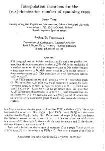
The Petersen Graph Embedded on a Klein Bottle. – Finally, we consider the graph (Figure 15), which is labelled and oriented as in Figure 11. On a Klein bottle, the number of patches equals (e – v) (= (m – 1)) and they
275
A THEOREM FOR COUNTING SPANNING TREES
are all independent. However, we shall select two simple generic cycles and discard one of the potential patches. The generic cycles chosen are 5 (edges 6 5 4 9 11) and 6 (edges 10 14 7 1 5). The analysis now proceeds as described (p. 273, l. col.) but the cycles are 'visible'. In fact, M could easily have been compiled directly by the 'cycle-overlap' method.
6 2
>
>
13
10
14
4
2
>
12 6
>
9
5
11
>
>
10
4 >
>
5
3
>
> >
5
6
>
>8