In this paper we present a new concept of program-size complexity. What train of
thought led us to it? Following [8, Sec. VI, p.7], think of a computer as decoding ...
A THEORY OF PROGRAM SIZE FORMALLY IDENTICAL TO INFORMATION THEORY Journal of the ACM 22 (1975), pp. 329–340 Gregory J. Chaitin1 IBM Thomas J. Watson Research Center Yorktown Heights, New York
Abstract A new definition of program-size complexity is made. H(A, B/C, D) is defined to be the size in bits of the shortest self-delimiting program for calculating strings A and B if one is given a minimal-size selfdelimiting program for calculating strings C and D. This differs from previous definitions: (1) programs are required to be self-delimiting, i.e. no program is a prefix of another, and (2) instead of being given C and D directly, one is given a program for calculating them that is minimal in size. Unlike previous definitions, this one has precisely the formal 1
G. J. Chaitin
2
properties of the entropy concept of information theory. For example, H(A, B) = H(A) + H(B/A) + O(1). Also, if a program of length k is assigned measure 2−k , then H(A) = − log2 (the probability that the standard universal computer will calculate A) + O(1).
Key Words and Phrases: computational complexity, entropy, information theory, instantaneous code, Kraft inequality, minimal program, probability theory, program size, random string, recursive function theory, Turing machine
CR Categories: 5.25, 5.26, 5.27, 5.5, 5.6
1. Introduction There is a persuasive analogy between the entropy concept of information theory and the size of programs. This was realized by the first workers in the field of program-size complexity, Solomonoff [1], Kolmogorov [2], and Chaitin [3,4], and it accounts for the large measure of success of subsequent work in this area. However, it is often the case that results are cumbersome and have unpleasant error terms. These ideas cannot be a tool for general use until they are clothed in a powerful formalism like that of information theory. This opinion is apparently not shared by all workers in this field (see Kolmogorov [5]), but it has led others to formulate alternative 1
c 1975, Association for Computing Machinery, Inc. General permisCopyright sion to republish, but not for profit, all or part of this material is granted provided that ACM’s copyright notice is given and that reference is made to the publication, to its date of issue, and to the fact that reprinting privileges were granted by permission of the Association for Computing Machinery. This paper was written while the author was a visitor at the IBM Thomas J. Watson Research Center, Yorktown Heights, New York, and was presented at the IEEE International Symposium on Information Theory, Notre Dame, Indiana, October 1974. Author’s present address: Rivadavia 3580, Dpto. 10A, Buenos Aires, Argentina.
A Theory of Program Size
3
definitions of program-size complexity, for example, Loveland’s uniform complexity [6] and Schnorr’s process complexity [7]. In this paper we present a new concept of program-size complexity. What train of thought led us to it? Following [8, Sec. VI, p.7], think of a computer as decoding equipment at the receiving end of a noiseless binary communications channel. Think of its programs as code words, and of the result of the computation as the decoded message. Then it is natural to require that the programs/code words form what is called an “instantaneous code,” so that successive messages sent across the channel (e.g. subroutines) can be separated. Instantaneous codes are well understood by information theorists [9–12]; they are governed by the Kraft inequality, which therefore plays a fundamental role in this paper. One is thus led to define the relative complexity H(A, B/C, D) of A and B with respect to C and D to be the size of the shortest selfdelimiting program for producing A and B from C and D. However, this is still not quite right. Guided by the analogy with information theory, one would like H(A, B) = H(A) + H(B/A) + ∆ to hold with an error term ∆ bounded in absolute value. But, as is shown in the Appendix, |∆| is unbounded. So we stipulate instead that H(A, B/C, D) is the size of the smallest self-delimiting program that produces A and B when it is given a minimal-size self-delimiting program for C and D. Then it can be shown that |∆| is bounded. In Sections 2–4 we define this new concept formally, establish the basic identities, and briefly consider the resulting concept of randomness or maximal entropy. We recommend reading Willis [13]. In retrospect it is clear that he was aware of some of the basic ideas of this paper, though he developed them in a different direction. Chaitin’s study [3,4] of the state complexity of Turing machines may be of interest, because in his formalism programs can also be concatenated. To compare the properties of our entropy function H with those it has in information theory, see [9–12]; to contrast its properties with those of previous definitions of programsize complexity, see [14]. Cover [15] and Gewirtz [16] use our new
4
G. J. Chaitin
definition. See [17–32] for other applications of information/entropy concepts.
2. Definitions X = {Λ, 0, 1, 00, 01, 10, 11, 000, . . .} is the set of finite binary strings, and X ∞ is the set of infinite binary strings. Henceforth we shall merely say “string” instead of “binary string,” and a string will be understood to be finite unless the contrary is explicitly stated. X is ordered as indicated, and |s| is the length of the string s. The variables p, q, s, and t denote strings. The variables α and ω denote infinite strings. αn is the prefix of α of length n. N = {0, 1, 2, . . .} is the set of natural numbers. The variables c, i, j, k, m, and n denote natural numbers. R is the set of positive rationals. The variable r denotes an element of R. We write “r.e.” instead of “recursively enumerable,” “lg” instead of “log2 ,” and sometimes “2 ↑ (x)” instead of “2x .” #(S) is the cardinality of the set S. Concrete Definition of a Computer. A computer C is a Turing machine with two tapes, a program tape and a work tape. The program tape is finite in length. Its leftmost square is called the dummy square and always contains a blank. Each of its remaining squares contains either a 0 or a 1. It is a read-only tape, and has one read head on it which can move only to the right. The work tape is two-way infinite and each of its squares contains either a 0, a 1, or a blank. It has one read-write head on it. At the start of a computation the machine is in its initial state, the program p occupies the whole program tape except for the dummy square, and the read head is scanning the dummy square. The work tape is blank except for a single string q whose leftmost symbol is being scanned by the read-write head. Note that q can be equal to Λ. In that case the read-write head initially scans a blank square. p can also be equal to Λ. In that case the program tape consists solely of the dummy square. See Figure 1. During each cycle of operation the machine may halt, move the read head of the program tape one square to the right, move the readwrite head of the work tape one square to the left or to the right, erase
A Theory of Program Size
0
5
0
1
1
0
1
0
6
Initial State ?
...
1
1
0
...
0
Figure 1. The start of a computation: p = 0011010 and q = 1100.
0
0
1
1
0
1
0 6
Halted ...
?
0
1
0
...
Figure 2. The end of a successful computation: C(p, q) = 010.
the square of the work tape being scanned, or write a 0 or a 1 on the square of the work tape being scanned. The the machine changes state. The action performed and the next state are both functions of the present state and the contents of the two squares being scanned, and are indicated in two finite tables with nine columns and as many rows as there are states. If the Turing machine eventually halts with the read head of the program tape scanning its rightmost square, then the computation is a success. If not, the computation is a failure. C(p, q) denotes the result of the computation. If the computation is a failure, then C(p, q) is undefined. If it is a success, then C(p, q) is the string extending to the right from the square of the work tape that is being scanned to the first blank square. Note that C(p, q) = Λ if the square of the work tape
6
G. J. Chaitin
being scanned is blank. See Figure 2. Definition of an Instantaneous Code. An instantaneous code is a set of strings S with the property that no string in S is a prefix of another. Abstract Definition of a Computer. A computer is a partial recursive function C : X × X → X with the property that for each q the domain of C(., q) is an instantaneous code; i.e. if C(p, q) is defined and p is a proper prefix of p0 , then C(p0 , q) is not defined. Theorem 2.1. The two definitions of a computer are equivalent. Proof. Why does the concrete definition satisfy the abstract one? The program must indicate within itself where it ends since the machine is not allowed to run off the end of the tape or to ignore part of the program. Thus no program for a successful computation is the prefix of another. Why does the abstract definition satisfy the concrete one? We show how a concrete computer C can simulate an abstract computer C 0 . The idea is that C should read another square of its program tape only when it is sure that this is necessary. Suppose C found the string q on its work tape. C then generates the r.e. set S = {p|C 0 (p, q) is defined} on its work tape. As it generates S, C continually checks whether or not that part p of the program that it has already read is a prefix of some known element s of S. Note that initially p = Λ. Whenever C finds that p is a prefix of an s ∈ S, it does the following. If p is a proper prefix of s, C reads another square of the program tape. And if p = s, C calculates C 0 (p, q) and halts, indicating this to be the result of the computation. Q.E.D. Definition of an Optimal Universal Computer. U is an optimal universal computer iff for each computer C there is a constant sim(C) with the following property: if C(p, q) is defined, then there is a p0 such that U(p0 , q) = C(p, q) and |p0 | ≤ |p| + sim(C). Theorem 2.2. There is an optimal universal computer U. Proof. U reads its program tape until it gets to the first 1. If U has read i 0’s, it then simulates Ci , the ith computer (i.e. the computer with the ith pair of tables in a recursive enumeration of all possible pairs of defining tables), using the remainder of the program tape as the program for Ci . Thus if Ci (p, q) is defined, then U(0i 1p, q) = Ci (p, q).
A Theory of Program Size
7
Hence U satisfies the definition of an optimal universal computer with sim(Ci ) = i + 1. Q.E.D. We somehow pick out a particular optimal universal computer U as the standard one for use throughout the rest of this paper. Definition of Canonical Programs, Complexities, and Probabilities. (a) The canonical program. s∗ = min p (U(p, Λ) = s). I.e. s∗ is the first element in the ordered set X of all strings that is a program for U to calculate s. (b) Complexities. HC (s) = min |p| (C(p, Λ) = s) (may be ∞), H(s) = HU (s), HC (s/t) = min |p| (C(p, t∗) = s) (may be ∞), H(s/t) = HU (s/t). (c) Probabilities. PC (s) =
P
2−|p| (C(p, Λ) = s),
P (s) = PU (s), PC (s/t) =
P
2−|p| (C(p, t∗ ) = s),
P (s/t) = PU (s/t). Remark on Nomenclature. There are two different sets of terminology for these concepts, one derived from computational complexity and the other from information theory. H(s) may be referred to as the information-theoretic or program-size complexity, and H(s/t) may be referred to as the relative information-theoretic or program-size complexity. Or H(s) and H(s/t) may be termed the algorithmic entropy and the conditional algorithmic entropy, respectively. Similarly, this field might be referred to as “information-theoretic complexity” or as “algorithmic information theory.”
G. J. Chaitin
8
Remark on the Definition of Probabilities. There is a very intuitive way of looking at the definition of PC . Change the definition of the computer C so that the program tape is infinite to the right, and remove the (now impossible) requirement for a computation to be successful that the rightmost square of the program tape is being scanned when C halts. Imagine each square of the program tape except for the dummy square to be filled with a 0 or a 1 by a separate toss of a fair coin. Then the probability that the result s is obtained when the work tape is initially blank is PC (s), and the probability that the result s is obtained when the work tape initially has t∗ on it is PC (s/t). Theorem 2.3. (a) H(s) ≤ HC (s) + sim(C), (b) H(s/t) ≤ HC (s/t) + sim(C), (c) s∗ 6= Λ, (d) s = U(s∗ , Λ), (e) H(s) = |s∗ |, (f) H(s) 6= ∞, (g) H(s/t) 6= ∞, (h) 0 ≤ PC (s) ≤ 1, (i) 0 ≤ PC (s/t) ≤ 1, (j) 1 ≥ (k) 1 ≥
P P
s
PC (s),
s
PC (s/t),
(l) PC (s) ≥ 2 ↑ (−HC (s)), (m) PC (s/t) ≥ 2 ↑ (−HC (s/t)), (n) 0 < P (s) < 1, (o) 0 < P (s/t) < 1,
A Theory of Program Size
9
(p) #({s|HC (s) < n}) < 2n , (q) #({s|HC (s/t) < n}) < 2n , (r) #({s|PC (s) > r}) < 1/r, (s) #({s|PC (s/t) > r}) < 1/r. Proof. These are immediate consequences of the definitions. Q.E.D. Definition of Tuples of Strings. Somehow pick out a particular recursive bijection b : X × X → X for use throughout the rest of this paper. The 1-tuple hs1 i is defined to be the string s1 . For n ≥ 2 the n-tuple hs1 , . . . , sn i is defined to be the string b(hs1 , . . . , sn−1 i, sn ). Extensions of the Previous Concepts to Tuples of Strings. (n ≥ 1, m ≥ 1). • HC (s1 , . . . , sn ) = HC (hs1 , . . . , sn i), • HC (s1 , . . . , sn /t1 , . . . , tm ) = HC (hs1 , . . . , sn i/ht1 , . . . , tm i), • H(s1 , . . . , sn ) = HU (s1 , . . . , sn ), • H(s1 , . . . , sn /t1 , . . . , tm ) = HU (s1 , . . . , sn /t1 , . . . , tm ), • PC (s1 , . . . , sn ) = PC (hs1 , . . . , sn i), • PC (s1 , . . . , sn /t1 , . . . , tm ) = PC (hs1 , . . . , sn i/ht1 , . . . , tm i), • P (s1 , . . . , sn ) = PU (s1 , . . . , sn ), • P (s1 , . . . , sn /t1 , . . . , tm ) = PU (s1 , . . . , sn /t1 , . . . , tm ). Definition of the Information in One Tuple of Strings About Another. (n ≥ 1, m ≥ 1). • IC (s1 , . . . , sn : t1 , . . . , tm ) = HC (t1 , . . . , tm ) − HC (t1 , . . . , tm /s1 , . . . , sn ), • I(s1 , . . . , sn : t1 , . . . , tm ) = IU (s1 , . . . , sn : t1 , . . . , tm ).
10
G. J. Chaitin
Extensions of the Previous Concepts to Natural Numbers. We have defined H, P , and I for tuples of strings. This is now extended to tuples each of whose elements may either be a string or a natural number. We do this by identifying the natural number n with the nth string (n = 0, 1, 2, . . .). Thus, for example, “H(n)” signifies “H(the nth element of X),” and “U(p, Λ) = n” stands for “U(p, Λ) = the nth element of X.”
3. Basic Identities This section has two objectives. The first is to show that H and I satisfy the fundamental inequalities and identities of information theory to within error terms of the order of unity. For example, the information in s about t is nearly symmetrical. The second objective is to show that P is approximately a conditional probability measure: P (t/s) and P (s, t)/P (s) are within a constant multiplicative factor of each other. The following notation is convenient for expressing these approximate relationships. O(1) denotes a function whose absolute value is less than or equal to c for all values of its arguments. And f ≈ g means that the functions f and g satisfy the inequalities cf ≥ g and f ≤ cg for all values of their arguments. In both cases c ∈ N is an unspecified constant. Theorem 3.1. (a) H(s, t) = H(t, s) + O(1), (b) H(s/s) = O(1), (c) H(H(s)/s) = O(1), (d) H(s) ≤ H(s, t) + O(1), (e) H(s/t) ≤ H(s) + O(1), (f) H(s, t) ≤ H(s) + H(t/s) + O(1), (g) H(s, t) ≤ H(s) + H(t) + O(1), (h) I(s : t) ≥ O(1),
A Theory of Program Size
11
(i) I(s : t) ≤ H(s) + H(t) − H(s, t) + O(1), (j) I(s : s) = H(s) + O(1), (k) I(Λ : s) = O(1), (l) I(s : Λ) = O(1). Proof. These are easy consequences of the definitions. The proof of Theorem 3.1(f) is especially interesting, and is given in full below. Also, note that Theorem 3.1(g) follows immediately from Theorem 3.1(f,e), and Theorem 3.1(i) follows immediately from Theorem 3.1(f) and the definition of I. Now for the proof of Theorem 3.1(f). We claim that there is a computer C with the following property. If U(p, s∗ ) = t and |p| = H(t/s) (i.e. if p is a minimal-size program for calculating t from s∗ ), then C(s∗ p, Λ) = hs, ti. By using Theorem 2.3(e,a) we see that HC (s, t) ≤ |s∗ p| = |s∗ | + |p| = H(s) + H(t/s), and H(s, t) ≤ HC (s, t) + sim(C) ≤ H(s) + H(t/s) + O(1). It remains to verify the claim that there is such a computer. C does the following when it is given the program s∗ p on its program tape and the string Λ on its work tape. First it simulates the computation that U performs when given the same program and work tapes. In this manner C reads the program s∗ and calculates s. Then it simulates the computation that U performs when given s∗ on its work tape and the remaining portion of C’s program tape. In this manner C reads the program p and calculates t from s∗ . The entire program tape has now been read, and both s and t have been calculated. C finally forms the pair hs, ti and halts, indicating this to be the result of the computation. Q.E.D. Remark. The rest of this section is devoted to showing that the “≤” in Theorem 3.1(f) and 3.1(i) can be replaced by “=.” The arguments used to do this are more probabilistic than information-theoretic in nature. Theorem 3.2. (Extension of the Kraft inequality condition for the existence of an instantaneous code). Hypothesis. Consider an effectively given list of finitely or infinitely many “requirements” hsk , nk i (k = 0, 1, 2, . . .) for the construction of a
12
G. J. Chaitin P
computer. The requirements are said to be “consistent” if 1 ≥ k 2 ↑ (−nk ), and we assume that they are consistent. Each requirement hsk , nk i requests that a program of length nk be “assigned” to the result sk . A computer C is said to “satisfy” the requirements if there are precisely as many programs p of length n such that C(p, Λ) = s as there are pairs hs, ni in the list of requirements. Such a C must have the P property that PC (s) = 2 ↑ (−nk ) (sk = s) and HC (s) = min nk (sk = s). Conclusion. There are computers that satisfy these requirements. Moreover, if we are given the requirements one by one, then we can simulate a computer that satisfies them. Hereafter we refer to the particular computer that the proof of this theorem shows how to simulate as the one that is “determined” by the requirements. Proof. (a) First we give what we claim is the (abstract) definition of a particular computer C that satisfies the requirements. In the second part of the proof we justify this claim. As we are given the requirements, we assign programs to results. Initially all programs for C are available. When we are given the requirement hsk , nk i we assign the first available program of length nk to the result sk (first in the ordering which X was defined to have in Section 2). As each program is assigned, it and all its prefixes and extensions become unavailable for future assignments. Note that a result can have many programs assigned to it (of the same or different lengths) if there are many requirements involving it. How can we simulate C? As we are given the requirements, we make the above assignments, and we simulate C by using the technique that was given in the proof of Theorem 2.1 for a concrete computer to simulate an abstract one. (b) Now to justify the claim. We must show that the above rule for making assignments never fails, i.e. we must show that it is never the case that all programs of the requested length are unavailable. The proof we sketch is due to N. J. Pippenger.
A Theory of Program Size
13
A geometrical interpretation is necessary. Consider the unit interval [0, 1). The kth program of length n (0 ≤ k < 2n ) corresponds to the interval [k2−n , (k + 1)2−n ). Assigning a program corresponds to assigning all the points in its interval. The condition that the set of assigned programs must be an instantaneous code corresponds to the rule that an interval is available for assignment iff no point in it has already been assigned. The rule we gave above for making assignments is to assign that interval [k2−n , (k + 1)2−n ) of the requested length 2−n that is available that has the smallest possible k. Using this rule for making assignments gives rise to the following fact. Fact. The set of those points in [0, 1) that are unassigned can always be expressed as the union of a finite number of intervals [ki 2 ↑ (−ni ), (ki + 1)2 ↑ (−ni )) with the following properties: ni > ni+1 , and (ki + 1)2 ↑ (−ni ) ≤ ki+1 2 ↑ (−ni+1 ). I.e. these intervals are disjoint, their lengths are distinct powers of 2, and they appear in [0, 1) in order of increasing length. We leave to the reader the verification that this fact is always the case and that it implies that an assignment is impossible only if the interval requested is longer than the total length of the unassigned part of [0, 1), i.e. only if the requirements are inconsistent. Q.E.D. Theorem 3.3. (Recursive “estimates” for HC and PC ). Consider a computer C. (a) The set of all true propositions of the form “HC (s) ≤ n” is r.e. Given t∗ one can recursively enumerate the set of all true propositions of the form “HC (s/t) ≤ n.” (b) The set of all true propositions of the form “PC (s) > r” is r.e. Given t∗ one can recursively enumerate the set of all true propositions of the form “PC (s/t) > r.” Proof. This is an easy consequence of the fact that the domain of C is an r.e. set. Q.E.D.
G. J. Chaitin
14
Remark. The set of all true propositions of the form “H(s/t) ≤ n” is not r.e.; for if it were r.e., it would easily follow from Theorems 3.1(c) and 2.3(q) that Theorem 5.1(f) is false, which is a contradiction. Theorem 3.4. For each computer C there is a constant c such that (a) H(s) ≤ − lg PC (s) + c, (b) H(s/t) ≤ − lg PC (s/t) + c. Proof. It follows from Theorem 3.3(b) that the set T of all true propositions of the form “PC (s) > 2−n ” is r.e., and that given t∗ one can recursively enumerate the set Tt of all true propositions of the form “PC (s/t) > 2−n .” This will enable us to use Theorem 3.2 to show that there is a computer C 0 with these properties: HC 0 (s) = d− lg PC (s)e + 1, PC 0 (s) = 2 ↑ (−d− lg PC (s)e),
(1)
HC 0 (s/t) = d− lg PC (s/t)e + 1, PC 0 (s/t) = 2 ↑ (−d− lg PC (s/t)e).
(2)
Here dxe denotes the least integer greater than x. By applying Theorem 2.3(a,b) to (1) and (2), we see that Theorem 3.4 holds with c = sim(C 0 ) + 2. How does the computer C 0 work? First of all, it checks whether it has been given Λ or t∗ on its work tape. These two cases can be distinguished, for by Theorem 2.3(c) it is impossible for t∗ to be equal to Λ. (a) If C 0 has been given Λ on its work tape, it enumerates T and simulates the computer determined by all requirements of the form hs, n + 1i (“PC (s) > 2−n ” ∈ T ). (3) Thus hs, ni is taken as a requirement iff n ≥ d− lg PC (s)e + 1. Hence the number of programs p of length n such that C 0 (p, Λ) = s is 1 if n ≥ d− lg PC (s)e+1 and is 0 otherwise, which immediately yields (1). However, we must check that the requirements (3) are consistent. 2−|p| (over all programs p we wish to assign to the result s) =
P
A Theory of Program Size
15 P
2 ↑ (−d− lg PC (s)e) < PC (s). Hence 2−|p| (over all p we wish to P assign) < s PC (s) ≤ 1 by Theorem 2.3(j). Thus the hypothesis of Theorem 3.2 is satisfied, the requirements (3) indeed determine a computer, and the proof of (1) and Theorem 3.4(a) is complete. (b) If C 0 has been given t∗ on its work tape, it enumerates Tt and simulates the computer determined by all requirements of the form hs, n + 1i (“PC (s/t) > 2−n ” ∈ Tt ). (4) Thus hs, ni is taken as a requirement iff n ≥ d− lg PC (s/t)e + 1. Hence the number of programs p of length n such that C 0 (p, t∗ ) = s is 1 if n ≥ d− lg PC (s/t)e + 1 and is 0 otherwise, which immediately yields (2). However, we must check that the requirements (4) are consistent. 2−|p| (over all programs p we wish to assign to the result s) = P 2 ↑ (−d− lg PC (s/t)e) < PC (s/t). Hence 2−|p| (over all p we P wish to assign) < s PC (s/t) ≤ 1 by Theorem 2.3(k). Thus the hypothesis of Theorem 3.2 is satisfied, the requirements (4) indeed determine a computer, and the proof of (2) and Theorem 3.4(b) is complete. Q.E.D.
P
Theorem 3.5. (a) For each computer C there is a constant c such that P (s) ≥ 2−c PC (s), P (s/t) ≥ 2−c PC (s/t). (b) H(s) = − lg P (s) + O(1), H(s/t) = − lg P (s/t) + O(1). Proof. Theorem 3.5(a) follows immediately from Theorem 3.4 using the fact that P (s) ≥ 2 ↑ (−H(s)) and P (s/t) ≥ 2 ↑ (−H(s/t)) (Theorem 2.3(l,m)). Theorem 3.5(b) is obtained by taking C = U in Theorem 3.4 and also using these two inequalities. Q.E.D. Remark. Theorem 3.4(a) extends Theorem 2.3(a,b) to probabilities. Note that Theorem 3.5(a) is not an immediate consequence of our weak definition of an optimal universal computer. Theorem 3.5(b) enables one to reformulate results about H as results concerning P , and vice versa; it is the first member of a trio of
G. J. Chaitin
16
formulas that will be completed with Theorem 3.9(e,f). These formulas are closely analogous to expressions in information theory for the information content of individual events or symbols [10, Secs. 2.3, 2.6, pp. 27–28, 34–37]. Theorem 3.6. (a) # ({p|U(p, Λ) = s & |p| ≤ H(s) + n}) ≤ 2 ↑ (n + O(1)). (b) # ({p|U(p, t∗ ) = s & |p| ≤ H(s/t) + n}) ≤ 2 ↑ (n + O(1)). Proof. This follows immediately from Theorem 3.5(b). Q.E.D. P Theorem 3.7. P (s) ≈ t P (s, t). Proof. On the one hand, there is a computer C such that C(p, Λ) = s P if U(p, Λ) = hs, ti. Thus PC (s) ≥ t P (s, t). Using Theorem 3.5(a), we P see that P (s) ≥ 2−c t P (s, t). On the other hand, there is a computer C such that C(p, Λ) = hs, si P if U(p, Λ) = s. Thus t PC (s, t) ≥ PC (s, s) ≥ P (s). Using Theorem P 3.5(a), we see that t P (s, t) ≥ 2−c P (s). Q.E.D. Theorem 3.8. There is a computer C and a constant c such that HC (t/s) = H(s, t) − H(s) + c. Proof. The set of all programs p such that U(p, Λ) is defined is r.e. Let pk be the kth program in a particular recursive enumeration of this set, and define sk and tk by hsk , tk i = U(pk , Λ). By Theorems P 3.7 and 3.5(b) there is a c such that 2 ↑ (H(s) − c) t P (s, t) ≤ 1 for all s. Given s∗ on its work tape, C simulates the computer Cs determined by the requirements htk , |pk | − |s∗ | + ci for k = 0, 1, 2, . . . such that sk = U(s∗ , Λ). Recall Theorem 2.3(d,e). Thus for each p such that U(p, Λ) = hs, ti there is a corresponding p0 such that C(p0 , s∗ ) = Cs (p0 , Λ) = t and |p0 | = |p| − H(s) + c. Hence HC (t/s) = H(s, t) − H(s) + c. However, we must check that the requirements for Cs are consistent. P 2 ↑ (−|p0 |) (over all programs p0 we wish to assign to any result P t) = 2 ↑ (−|p| + H(s) − c) (over all p such that U(p, Λ) = hs, ti) = P 2 ↑ (H(s)−c) t P (s, t) ≤ 1 because of the way c was chosen. Thus the hypothesis of Theorem 3.2 is satisfied, and these requirements indeed determine Cs . Q.E.D. Theorem 3.9.
A Theory of Program Size
17
(a) H(s, t) = H(s) + H(t/s) + O(1), (b) I(s : t) = H(s) + H(t) − H(s, t) + O(1), (c) I(s : t) = I(t : s) + O(1), (d) P (t/s) ≈ P (s, t)/P (s), (e) H(t/s) = lg P (s)/P (s, t) + O(1), (f) I(s : t) = lg P (s, t)/P (s)P (t) + O(1). Proof. (a) Theorem 3.9(a) follows immediately from Theorems 3.8, 2.3(b), and 3.1(f). (b) Theorem 3.9(b) follows immediately from Theorem 3.9(a) and the definition of I(s : t). (c) Theorem 3.9(c) follows immediately from Theorems 3.9(b) and 3.1(a). (d,e) Theorem 3.9(d,e) follows immediately from Theorems 3.9(a) and 3.5(b). (f) Theorem 3.9(f) follows immediately from Theorems 3.9(b) and 3.5(b). Q.E.D. Remark. We thus have at our disposal essentially the entire formalism of information theory. Results such as these can now be obtained effortlessly: • H(s1 ) ≤ H(s1 /s2 ) + H(s2/s3 ) + H(s3 /s4 ) + H(s4 ) + O(1), • H(s1 , s2 , s3 , s4 ) = H(s1 /s2 , s3 , s4 ) + H(s2 /s3 , s4 ) + H(s3 /s4 ) + H(s4 ) + O(1). However, there is an interesting class of identities satisfied by our H function that has no parallel in information theory. The simplest of these is H(H(s)/s) = O(1) (Theorem 3.1(c)), which with Theorem
G. J. Chaitin
18
3.9(a) immediately yields H(s, H(s)) = H(s) + O(1). This is just one pair of a large family of identities, as we now proceed to show. Keeping Theorem 3.9(a) in mind, consider modifying the computer C used in the proof of Theorem 3.1(f) so that it also measures the lengths H(s) and H(t/s) of its subroutines s∗ and p, and halts indicating hs, t, H(s), H(t/s)i to be the result of the computation instead of hs, ti. It follows that H(s, t) = H(s, t, H(s), H(t/s)) + O(1) and H(H(s), H(t/s)/s, t) = O(1). In fact, it is easy to see that H(H(s), H(t), H(t/s), H(s/t), H(s, t)/s, t) = O(1), which implies H(I(s : t)/s, t) = O(1). And of course these identities generalize to tuples of three or more strings.
4. A Random Infinite String The undecidability of the halting problem is a fundamental theorem of recursive function theory. In algorithmic information theory the corresponding theorem is as follows: The base-two representation of the probability that U halts is a random (i.e. maximally complex) infinite string. In this section we formulate this statement precisely and prove it. Theorem 4.1. (Bounds on the complexity of natural numbers). (a)
P
n
2−H(n) ≤ 1.
Consider a recursive function f : N → N. (b) If (c) If
P P
n
2−f (n) diverges, then H(n) > f (n) infinitely often.
n
2−f (n) converges, then H(n) ≤ f (n) + O(1).
Proof. (a) By Theorem 2.3(l,j), P
P
n
2−H(n) ≤
P
n
P (n) ≤ 1.
(b) If n 2−f (n) diverges, and H(n) ≤ f (n) held for all but finitely P many values of n, then n 2−H(n) would also diverge. But this would contradict Theorem 4.1(a), and thus H(n) > f (n) infinitely often.
A Theory of Program Size P
19 P
(c) If n 2−f (n) converges, there is an n0 such that n≥n0 2−f (n) ≤ 1. By Theorem 3.2 there is a computer C determined by the requirements hn, f (n)i (n ≥ n0 ). Thus H(n) ≤ f (n) + sim(C) for all n ≥ n0 . Q.E.D. Theorem 4.2. (Maximal complexity finite and infinite strings). (a) max H(s) (|s| = n) = n + H(n) + O(1). (b) # ({s| |s| = n & H(s) ≤ n + H(n) − k}) ≤ 2 ↑ (n − k + O(1)). (c) Imagine that the infinite string α is generated by tossing a fair coin once for each if its bits. Then, with probability one, H(αn ) > n for all but finitely many n. Proof. (a,b) Consider a string s of length n. By Theorem 3.9(a), H(s) = H(n, s)+O(1) = H(n)+H(s/n)+O(1). We now obtain Theorem 4.2(a,b) from this estimate for H(s). There is a computer C such that C(p, |p|∗) = p for all p. Thus H(s/n) ≤ n + sim(C), and H(s) ≤ n + H(n) + O(1). On the other hand, by Theorem 2.3(q), fewer than 2n−k of the s satisfy H(s/n) < n − k. Hence fewer than 2n−k of the s satisfy H(s) < n − k + H(n) + O(1). Thus we have obtained Theorem 4.2(a,b). (c) Now for the proof of Theorem 4.2(c). By Theorem 4.2(b), at most a fraction of 2 ↑ (−H(n) + c) of the strings s of length n satisfy H(s) ≤ n. Thus the probability that α satisfies H(αn ) ≤ n is P ≤ 2 ↑ (−H(n) + c). By Theorem 4.1(a), n 2 ↑ (−H(n) + c) converges. Invoking the Borel-Cantelli lemma, we obtain Theorem 4.2(c). Q.E.D. Definition of Randomness. A string s is random iff H(s) is approximately equal to |s| + H(|s|). An infinite string α is random iff ∃c ∀n H(αn ) > n − c. Remark. In the case of infinite strings there is a sharp distinction between randomness and nonrandomness. In the case of finite strings it is a matter of degree. To the question “How random is s?” one must reply indicating how close H(s) is to |s| + H(|s|).
G. J. Chaitin
20
C. P. Schnorr (private communication) has shown that this complexity-based definition of a random infinite string and P. Martin-L¨of’s statistical definition of this concept [7, pp. 379–380] are equivalent. Definition of Base-Two Representations. The base-two representation of a real number x ∈ (0, 1] is that unique string b1 b2 b3 . . . P with infinitely many 1’s such that x = k bk 2−k . P Definition of the Probability ω that U Halts. ω = s P (s) = P −|p| 2 (U(p, Λ) is defined). By Theorem 2.3(j,n), ω ∈ (0, 1]. Therefore the real number ω has a base-two representation. Henceforth ω denotes both the real number and its base-two representation. Similarly, ωn denotes a string of length n and a rational number m/2n with the property that ω > ωn and ω − ωn ≤ 2−n . Theorem 4.3. (Construction of a random infinite string). (a) There is a recursive function w : N → R such that w(n) ≤ w(n + 1) and ω = limn→∞ w(n). (b) ω is random. (c) There is a recursive predicate D : N ×N ×N → {true, false} such that the k-th bit of ω is a 1 iff ∃i ∀j D(i, j, k) (k = 0, 1, 2, . . .). Proof. (a) {p|U(p, Λ) is defined} is r.e. Let pk (k = 0, 1, 2, . . .) denote the kth p in a particular recursive enumeration of this set. Let w(n) = P k≤n 2 ↑ (−|pk |). w(n) tends monotonically to ω from below, which proves Theorem 4.3(a). (b) In view of the fact that ω > ωn ≥ ω − 2−n (see the definition of ω), if one is given ωn one can find an m such that ω ≥ w(m) > ωn ≥ ω − 2−n . Thus ω − w(m) < 2−n , and {pk |k ≤ m} contains all programs p of length less than or equal to n such that U(p, Λ) is defined. Hence {U(pk , Λ)|k ≤ m & |pk | ≤ n} = {s|H(s) ≤ n}. It follows there is a computer C with the property that if U(p, Λ) = ωn , then C(p, Λ) equals the first string s such that H(s) > n. Thus n < H(s) ≤ H(ωn ) + sim(C), which proves Theorem 4.3(b).
A Theory of Program Size
21
(c) To prove Theorem 4.3(c), define D as follows: D(i, j, k) iff j ≥ i implies the kth bit of the base-two representation of w(j) is a 1. Q.E.D.
5. Appendix. The Traditional Concept of Relative Complexity In this Appendix programs are required to be self-delimiting, but the relative complexity H(s/t) of s with respect to t will now mean that one is directly given t, instead of being given a minimal-size program for t. The standard optimal universal computer U remains the same as before. H and P are redefined as follows: • HC (s/t) = min |p| (C(p, t) = s) (may be ∞), • HC (s) = HC (s/Λ), • H(s/t) = HU (s/t), • H(s) = HU (s), • PC (s/t) =
P
2−|p| (C(p, t) = s),
• PC (s) = PC (s/Λ), • P (s/t) = PU (s/t), • P (s) = PU (s). These concepts are extended to tuples of strings and natural numbers as before. Finally, ∆(s, t) is defined as follows: • H(s, t) = H(s) + H(t/s) + ∆(s, t). Theorem 5.1. (a) H(s, H(s)) = H(s) + O(1), (b) H(s, t) = H(s) + H(t/s, H(s)) + O(1),
G. J. Chaitin
22 (c) −H(H(s)/s) − O(1) ≤ ∆(s, t) ≤ O(1), (d) ∆(s, s) = O(1), (e) ∆(s, H(s)) = −H(H(s)/s) + O(1), (f) H(H(s)/s) 6= O(1). Proof.
(a) On the one hand, H(s, H(s)) ≤ H(s) + c because a minimal-size program for s also tells one its length H(s), i.e. because there is a computer C such that C(p, Λ) = hU(p, Λ), |p|i if U(p, Λ) is defined. On the other hand, obviously H(s) ≤ H(s, H(s)) + c. (b) On the one hand, H(s, t) ≤ H(s) + H(t/s, H(s)) + c follows from Theorem 5.1(a) and the obvious inequality H(s, t) ≤ H(s, H(s))+ H(t/s, H(s)) + c. On the other hand, H(s, t) ≥ H(s) + H(t/s, H(s)) − c follows from the inequality H(t/s, H(s)) ≤ H(s, t) − H(s) + c analogous to Theorem 3.8 and obtained by adapting the methods of Section 3 to the present setting. (c) This follows from Theorem 5.1(b) and the obvious inequality H(t/s, H(s)) − c ≤ H(t/s) ≤ H(H(s)/s) + H(t/s, H(s)) + c. (d) If t = s, H(s, t) − H(s) − H(t/s) = H(s, s) − H(s) − H(s/s) = H(s) − H(s) + O(1) = O(1), for obviously H(s, s) = H(s) + O(1) and H(s/s) = O(1). (e) If t = H(s), H(s, t) − H(s) − H(t/s) = H(s, H(s)) − H(s) − H(H(s)/s) = −H(H(s)/s) + O(1) by Theorem 5.1(a). (f) The proof is by reductio ad absurdum. Suppose on the contrary that H(H(s)/s) < c for all s. First we adapt an idea of A. R. Meyer and D. W. Loveland [6, pp. 525–526] to show that there is a partial recursive function f : X → N with the property that if f (s) is defined it is equal to H(s) and this occurs for infinitely many values of s. Then we obtain the desired contradiction by showing that such a function f cannot exist.
A Theory of Program Size
23
Consider the set Ks of all natural numbers k such that H(k/s) < c and H(s) ≤ k. Note that min Ks = H(s), #(Ks ) < 2c , and given s one can recursively enumerate Ks . Also, given s and #(Ks ) one can recursively enumerate Ks until one finds all its elements, and, in particular, its smallest element, which is H(s). Let m = lim sup #(Ks ), and let n be such that |s| ≥ n implies #(Ks ) ≤ m. Knowing m and n one calculates f (s) as follows. First one checks if |s| < n. If so, f (s) is undefined. If not, one recursively enumerates Ks until m of its elements are found. Because of the way n was chosen, Ks cannot have more than m elements. If it has less than m, one never finishes searching for m of them, and so f (s) is undefined. However, if #(Ks ) = m, which occurs for infinitely many values of s, then one eventually realizes all of them have been found, including f (s) = min Ks = H(s). Thus f (s) is defined and equal to H(s) for infinitely many values of s. It remains to show that such an f is impossible. As the length of s increases, H(s) tends to infinity, and so f is unbounded. Thus given n and H(n) one can calculate a string sn such that H(n) + n < f (sn ) = H(sn ), and so H(sn /n, H(n)) is bounded. Using Theorem 5.1(b) we obtain H(n) + n < H(sn ) ≤ H(n, sn ) + c0 ≤ H(n) + H(sn /n, H(n)) + c00 ≤ H(n) + c000 , which is impossible for n ≥ c0000 . Thus f cannot exist, and our initial assumption that H(H(s)/s) < c for all s must be false. Q.E.D. Remark. Theorem 5.1 makes it clear that the fact that H(H(s)/s) is unbounded implies that H(t/s) is less convenient to use than H(t/s, H(s)). In fact, R. Solovay (private communication) has announced that max H(H(s)/s) taken over all strings s of length n is asymptotic to lg n. The definition of the relative complexity of s with respect to t given in Section 2 is equivalent to H(s/t, H(t)).
Acknowledgments The author is grateful to the following for conversations that helped to crystallize these ideas: C. H. Bennett, T. M. Cover, R. P. Daley,
24
G. J. Chaitin
M. Davis, P. Elias, T. L. Fine, W. L. Gewirtz, D. W. Loveland, A. R. Meyer, M. Minsky, N. J. Pippenger, R. J. Solomonoff, and S. Winograd. The author also wishes to thank the referees for their comments.
References [1] Solomonoff, R. J. A formal theory of inductive inference. Inform. and Contr. 7 (1964), 1–22, 224–254. [2] Kolmogorov, A. N. Three approaches to the quantitative definition of information. Problems of Inform. Transmission 1, 1 (Jan.–March 1965), 1–7. [3] Chaitin, G. J. On the length of programs for computing finite binary sequences. J. ACM 13, 4 (Oct. 1966), 547–569. [4] Chaitin, G. J. On the length of programs for computing finite binary sequences: Statistical considerations. J. ACM 16, 1 (Jan. 1969), 145–159. [5] Kolmogorov, A. N. On the logical foundations of information theory and probability theory. Problems of Inform. Transmission 5, 3 (July–Sept. 1969), 1–4. [6] Loveland, D. W. A variant of the Kolmogorov concept of complexity. Inform. and Contr. 15 (1969), 510–526. [7] Schnorr, C. P. Process complexity and effective random tests. J. Comput. and Syst. Scis. 7 (1973), 376–388. [8] Chaitin, G. J. On the difficulty of computations. IEEE Trans. IT-16 (1970), 5–9. [9] Feinstein, A. Foundations of Information Theory. McGrawHill, New York, 1958. [10] Fano, R. M. Transmission of Information. Wiley, New York, 1961.
A Theory of Program Size
25
[11] Abramson, N. Information Theory and Coding. McGraw-Hill, New York, 1963. [12] Ash, R. Information Theory. Wiley-Interscience, New York, 1965. [13] Willis, D. G. Computational complexity and probability constructions. J. ACM 17, 2 (April 1970), 241–259. [14] Zvonkin, A. K. and Levin, L. A. The complexity of finite objects and the development of the concepts of information and randomness by means of the theory of algorithms. Russ. Math. Survs. 25, 6 (Nov.–Dec. 1970), 83–124. [15] Cover, T. M. Universal gambling schemes and the complexity measures of Kolmogorov and Chaitin. Rep. No. 12, Statistics Dep., Stanford U., Stanford, Calif., 1974. Submitted to Ann. Statist. [16] Gewirtz, W. L. Investigations in the theory of descriptive complexity. Ph.D. Thesis, New York University, 1974 (to be published as a Courant Institute rep.). [17] Weiss, B. The isomorphism problem in ergodic theory. Bull. Amer. Math. Soc. 78 (1972), 668–684. [18] R´ enyi, A. Foundations of Probability. Holden-Day, San Francisco, 1970. [19] Fine, T. L. Theories of Probability: An Examination of Foundations. Academic Press, New York, 1973. [20] Cover, T. M. On determining the irrationality of the mean of a random variable. Ann. Statist. 1 (1973), 862–871. [21] Chaitin, G. J. Information-theoretic computational complexity. IEEE Trans. IT-20 (1974), 10–15. [22] Levin, M. Mathematical Logic for Computer Scientists. Rep. TR-131, M.I.T. Project MAC, 1974, pp. 145–147,153.
26
G. J. Chaitin
[23] Chaitin, G. J. Information-theoretic limitations of formal systems. J. ACM 21, 3 (July 1974), 403–424. [24] Minsky, M. L. Computation: Finite and Infinite Machines. Prentice-Hall, Englewood Cliffs, N.J., 1967, pp. 54, 55, 66. [25] Minsky, M. and Papert, S. Perceptrons: An Introduction to Computational Geometry. M.I.T. Press, Cambridge, Mass. 1969, pp. 150–153. [26] Schwartz, J. T. On Programming: An Interim Report on the SETL Project. Installment I: Generalities. Lecture Notes, Courant Institute, New York University, New York, 1973, pp. 1–20. [27] Bennett, C. H. Logical reversibility of computation. IBM J. Res. Develop. 17 (1973), 525–532. [28] Daley, R. P. The extent and density of sequences within the minimal-program complexity hierarchies. J. Comput. and Syst. Scis. (to appear). [29] Chaitin, G. J. Information-theoretic characterizations of recursive infinite strings. Submitted to Theoretical Comput. Sci. [30] Elias, P. Minimum times and memories needed to compute the values of a function. J. Comput. and Syst. Scis. (to appear). [31] Elias, P. Universal codeword sets and representations of the integers. IEEE Trans. IT (to appear). [32] Hellman, M. E. The information theoretic approach to cryptography. Center for Systems Research, Stanford U., Stanford, Calif., 1974. [33] Chaitin, G. J. Randomness and mathematical proof. Sci. Amer. 232, 5 (May 1975), in press. (Note. Reference [33] is not cited in the text.)
A Theory of Program Size
Received April 1974; Revised December 1974
27