1443
A three-dimensional model to simulate joint networks in layered rocks Jean-Yves Josnin, Hervé Jourde, Pascal Fénart, and Pascal Bidaux
Abstract: Modelling the discontinuity network of fractured reservoirs may be addressed (1) by purely stochastic means, (2) with a fractal approach, or (3) using mechanical parameters describing the spatial organisation of fracture systems. Our paper presents an approach where the geometrical properties of the fracture networks are incorporated in the form of both statistical and mechanical rules. This type of approach is particularly suitable to model stratified fractured rock masses comprising two orthogonal families of joints and a family of sedimentary discontinuities. Their geometrical arrangement is governed by two kinds of rules based on (1) statistical parameters such as the mean, standard deviation of joint length and of bed thickness, both determined by field observations, and (2) geometrical parameters that result from genetic processes inferred from field observations and analogue experiments on the nucleation and propagation mechanisms of joints. Using these parameters, we generate realistic networks in terms of the relative position of joints that control the overall network connectivity: the model enables all combinations of joint spacing and vertical persistence for orthogonal patterns ranging from ladder type to grid type patterns. It also integrates the concept of mechanical “saturation” of a bed, thereby permitting the generation of both “saturated” and “unsaturated” networks. Résumé : La modélisation des réseaux de discontinuités dans les réservoirs fracturés peut être réalisée (1) de façon purement stochastique ; (2) à partir d’une approche fractale ; (3) en utilisant des lois mécaniques qui décrivent l’organisation spatiale du système de fractures. Cet article présente une approche dans laquelle les propriétés des réseaux de fractures sont prises en compte en utilisant à la fois des lois mécaniques et statistiques. Ce type d’approche est particulièrement bien adapté pour la modélisation de masses rocheuses sédimentaires stratifiées affectées par deux familles de diaclases orthogonales. Le modèle présenté simule des réseaux de discontinuités comprenant des interfaces stratigraphiques et des diaclases d’origine tectonique. Leur arrangement géométrique est contrôlé par deux types de lois basées sur (1) des paramètres statistiques comme la moyenne et l’écart-type des longueurs de diaclases ou de l’épaisseur des strates, ceux ci résultant de mesures classiques sur le terrain; (2) des paramètres géométriques liés aux processus de génération des réseaux, ceux ci étant déterminés à partir de données de terrain et d’expériences analogiques d’initiation et de propagation de diaclases. L’utilisation de ces paramètres permet la génération de réseaux réalistes en terme de position relative des diaclases dans l’espace, cette dernière contrôlant la connectivité globale du réseau : le modèle permet de reproduire toutes les configurations de réseaux de diaclases orthogonales depuis les réseaux « en échelle » jusqu’au réseaux « en grille ». Le modèle permet en effet de générer des réseaux pour lesquels la persistance verticale des diaclases à travers les interfaces stratigraphiques ainsi que l’espacement entre les diaclases peuvent être ajustés. Ce modèle intègre également le concept de « saturation » mécanique d’une strate, permettant ainsi la génération de réseaux « saturés » et « non saturés ». Josnin et al.
1455
Introduction The past forty years have given rise to new technological challenges like the exploitation of geothermal energy or the
assessment of sites for nuclear waste repositories, leading to an increasing interest in modelling the hydraulic behaviour of fractured rock masses. For such rock masses, the fluid flow behaviour mainly depends on the pattern of the joint
Received 10 January 2002. Accepted 12 July 2002. Published on the NRC Research Press Web site at http://cjes.nrc.ca on 30 September 2002. Paper handled by Associate Editor S. Hanmer. J.-Y. Josnin.1,2 Laboratoire Magmas et Volcans — Equipe Volcanologie, UMR 6524 du CNRS, Université Clermont-Ferrand II, 5 rue Kessler, F-63038 Clermont-Ferrand, France. H. Jourde and P. Bidaux.3 Laboratoire Hydrosciences, UMR 5569 du CNRS, Université Montpellier II, Maison des Sciences de l’Eau, 300 avenue E. Jeanbrau, F-34095 Montpellier CEDEX 05, France. Pascal Fénart. Centre des Matériaux de Grande Diffusion, Ecole des Mines d’Alès, 6 avenue de Clavières, F-30319 Alès CEDEX, France. 1
Present address: Laboratoire de Géologie et Hydrogéologie des Aquifères de Montagne, Université de Savoie, Domaine Scientifique, F-73376 Le Bourget-du-Lac CEDEX, France. 2 Corresponding author (e-mail:
[email protected]). 3 Present address: PERENCO S.A. 23–25, rue Dumont Durville, 75116 Paris, France. Can. J. Earth Sci. 39: 1443–1455 (2002)
DOI: 10.1139/E02-043
© 2002 NRC Canada
1444
network and on the hydraulic conductivity of fractures. Two fundamental approaches were taken to model this hydraulic behaviour: Initially, methodologies were formulated to determine whether a fractured rock mass behaved as a continuum (Snow 1979; Long et al. 1982; Long and Witherspoon 1985) and to compute equivalent hydraulic parameters for an elementary representative volume. This allowed the application of porous media numerical modelling, but a major difficulty remained: depending on the geometrical characteristics of the network, such an elementary representative volume may not exist (De Marsily 1985; Pavlovic 1998; Panda and Kulatilake 1999). More recently, with increasing computing capacity, it becomes possible to generate networks of discontinuities numerically and to simulate flows in these networks. Earlier models using this approach were based on fracture networks described either as purely stochastic (Long and Billaux 1987; Chiles 1988; Cacas 1989) or as fractal (Velde et al. 1991; Acuna and Yortsos 1995). To obtain more realistic simulations of fracture networks, the latter models included an increasing number of geometrical parameters (Bruel 1990; Bourgine et al. 1995; Gringarten 1996; Rawnsley and Swaby 1996; Cacas et al. 1997; Gringarten 1998). Most of these models are normally used to solve flow or stability problems. They generally simulate discontinuity networks in crystalline or metamorphic rocks adequately, but are not appropriate for stratified rock masses. These models do not account for the relative arrangement of fractures controlling the overall network connectivity because they fail to represent the complex intersection relations between discontinuity families, which result from various genetic processes at different tectonic stages. This observation lead to the development of a new category of models that consider (1) the geological genesis of the fractures, (2) the size and shape of the blocks delimited by the fractures, (3) the fracture termination type (Gervais et al. 1995), and (4) both geomechanics and flow simulation (Bourne et al. 2001). In the present approach, we do not focus on the flow properties of the fracture networks but on the description of a hierarchical model that reflects the genetic mechanism of joint formation. The network simulation is performed within a sequential and conditional generation of successive joint sets, which leads to a more realistic representation of geometrical relations between the sets of discontinuities within the rock mass. We present a three-dimensional hierarchical model based on the network modelling approach mentioned previously. Numerous field observations focus on the geometrical parameters and spatial arrangement of joints in tabular sedimentary rock masses (Pollard and Aydin 1988; Huang and Angelier 1989; Rives 1992; Narr and Suppe 1991; Gross 1993; Auzias 1996; Becker and Gross 1996; Pascal et al. 1997). Moreover, laboratory studies with analogue simulations (Rives et al. 1992 and 1994; Wu and Pollard 1995) and theoretical development of numerical modelling (Segall and Pollard 1980, 1983; Renshaw and Pollard 1994) give insights into the mechanisms that govern the joint nucleation and propagation in these media. We have, therefore, attempted to develop a model that simulates discontinuity networks composed of two orthogonal joint sets normal to bedding in tabular sedimentary rock masses. We first present the mechanisms for joint nucleation and propagation in sedimentary rock masses and how they were implemented in the numerical model. Then, we simulate a
Can. J. Earth Sci. Vol. 39, 2002
number of fracture networks to illustrate the range of geometries the model can generate and assess the model’s sensitivity to the main input parameters. Finally, we perform a simulation of a natural joint network located in the Swiss Jura.
Genetic and geometric characterization of discontinuity networks The model aims at simulating discontinuity networks that comprise two orthogonal families of joints in the presence of sedimentary discontinuities. Joints are defined as opening mode fractures, i.e., fractures formed under tensile stress without any shearing component (Pollard and Aydin 1988). This category of discontinuities is characterized by trace lengths that may span from a few millimetres to several metres, a rectilinear shape, and small apertures with respect to their length. They are typical of networks in tabular sedimentary rock masses. The statistical parameters of a fracture system include the orientation, the trace length, the density, as well as the shape of the fractures. These parameters are necessary to define the spatial organisation of every joint set. Genetic considerations focus on the chronology of fracture set formation, which is sequential and conditional, i.e., depending on the presence of other joints. Knowledge of this chronology permits definition of geometrical relationships between sets of discontinuities and the fracture termination types observed in the field. Joint shape Joints initiate on material discontinuities or flaws (fossils, mineral inclusions, bedding parallel planes, grain boundaries) that act as stress concentrators. They propagate in a pseudo-radial manner from this point and are perpendicular to bedding (Pollard and Aydin 1988). In an ideal homogeneous medium, where growth is not stopped by discontinuities, joints would have circular to elliptical shapes with bedding-parallel long axes (Pollard and Aydin 1988; Petit et al. 1994). However, in layered rocks, vertical growth is limited by sedimentary discontinuities that act as mechanical barriers within the rock mass (Helgelson and Aydin 1991), and horizontal growth of joints may be limited by mechanical interactions with other joints. As a consequence, in sedimentary rock masses, joints are more or less rectangular in shape (Fig. 1). With a rectangular shape, the dimensions of single joints may be defined by an aspect ratio of maximum height (H) over maximum length (L). Field measurements in a sandstone rock mass (Petit et al. 1994) show that this ratio may range between 0.001 and 0.8, most of the values being around 0.5.
Geometrical characteristics of tectonic joint sets A joint set is defined as a system of joints that present a similar orientation. The spatial density of a set is generally determined by length and spacing distributions inferred from outcrop measurements. Numerous field studies demonstrate that statistical distribution laws as the power-law, log-normal, normal, and negative exponential laws can approximate length and spacing distributions. In sedimentary rock masses, joint length is generally characterized by a log-normal distribution © 2002 NRC Canada
Josnin et al. Fig. 1. Joints in stratified sedimentary rocks. They present roughly rectangular shape with H their height and L their length.
(Razack 1982; Malmanger and Teufel 1997). For a given layer thickness, it has been demonstrated experimentally (Rives et al. 1992) and observed in the field (Renshaw and Park 1997) that the spacing distribution of a joint set evolves from a negative exponential, through a log-normal, to a normal distribution as joint density increases. The observation that spacing follows a normal distribution for a maximum density of fractures is interpreted to reflect the development of all joints that could potentially develop. In this case, the layer is referred to as saturated (Rives et al. 1992; Wu and Pollard 1995; Renshaw 1997). In a homogeneous rock, within an isotropic stress field, joint propagation in a layer induces a decrease of the tensile stress magnitude in a zone around the joint. This zone is described as a relaxation zone in which the development of a preexisting joint, or the initiation of a new joint, is inhibited (Price and Cosgrove 1990; Rives 1992; Becker and Gross 1996; Bai and Pollard 2000) and will be referred to as shadow zone in the remaining of the paper. In areas of low tectonic strain, it has been demonstrated that the average joint spacing of one set within a bed is related to layer thickness by a positive linear relationship (Novikova 1947; Mc Quillan 1973; Ladeira and Price 1981; Huang and Angelier 1989; Wu and Pollard 1995; Bai and Pollard 2000). This observation is consistent with the concept of a shadow zone: when saturation is reached, the mean spacing decreases to finally equal the shadow zone width value. Rives (1992) verified this intrinsic joint set property with two-dimensional random numerical simulations of joint sets, whose development had been constrained by a shadow zone associated to each joint. Relationships between orthogonal joint sets Horizontal traces of orthogonal joint sets form different patterns depending on their crosscutting and abutting relationships (Rives et al. 1992). Generally, different joint sets do not form during the same geological event (Dyer 1988; Rives 1992; Bai and Gross 1999). The discontinuities of the first set may act as mechanical barriers for the second set of joints and thus limit their propagation. The percentage of abutting fractures depends both on the mechanical properties of the discontinuities acting as a mechanical barrier, and on the level of energy available for joint propagation. More generally, the ability for a fracture to cross a boundary depends on (1) the length of the fracture (which controls the
1445
size of the stress concentration), (2) the cohesion of the boundary, (3) the coefficient of friction along the boundary, and (4) the overburden stress (Renshaw and Pollard 1995). This percentage may be estimated by a stopping coefficient defined as the percentage of the joints of the second set that are stopped by a joint of the first set, versus the total number of joints of the second set. Relationships between sedimentary discontinuities and tectonic joints Field observations show that joints may be limited to one layer or may crosscut sedimentary discontinuities (Pollard and Aydin 1988). Similar to intersecting tectonic joint sets, we consider a stopping coefficient to describe the relationship between sedimentary discontinuities and tectonic joints. This coefficient is defined as the probability for tectonic joints to crosscut sedimentary discontinuities. Depending on whether sedimentary discontinuities act as barrier (low coefficient value) or not (high coefficient value), joints may penetrate one or more strata. When a joint plane crosscuts a mechanical barrier, fractographic analyses of the surface of the joint plane (plumose structures) show that a re-initialization of a new coplanar joint surface occurs at the interface (Joonnekindt 1994; Cortès 1995). The new coplanar joint is referred to as daughter joint. This phenomenon has been observed both in the field (Helgelson and Aydin 1991) and during experiments (Joonnekindt 1994; Cortes 1995). This allows a horizontal growth for the parent joint independent from that of the daughter joint, i.e., mechanical interactions with other joints will be considered independently within each bed when a joint crosscuts several consecutive layers.
Simulation of a discontinuity network Schematically, the generation of the network may be broken down into the steps presented in Fig. 2, which illustrates how the geometrical and genetic concepts are applied. See Appendix A for nomenclature. Generating sedimentary discontinuities After defining the rock mass dimensions (width and length), the program assumes that the layers are horizontal (tabular conditions) and that every layer represents a distinct mechanical unit called a bed. The sedimentary discontinuities are treated like mechanical interfaces, i.e., surfaces separating two layers that can have different mechanical properties. The thickness distribution is considered as log-normal, which is assumed to be a correct representation of the reality. The mean and standard deviation of this distribution, as well as the number of strata, are input parameters. Initiation and horizontal propagation of joints of the first set The number of initiating flaws used by the model to generate joints is an input parameter. For the generation of the first set, the initiating flaws are randomly distributed over the whole domain, each assigned to a bed (Z coordinate) within which it starts its development (X and Y coordinates). The length of each joint is randomly determined from a log-normal © 2002 NRC Canada
1446
Can. J. Earth Sci. Vol. 39, 2002
Fig. 2. The model. (a) Algorithm describing the different steps of the model. (b) Visualisation of a simulation.
distribution, the mean (Lm) and standard deviation (Lsd) of this distribution being input parameters. The code does not simulate joint propagation, but accounts for the previously defined physical laws that describe this mechanism such that the final length and tip position of the joints be realistically reproduced. The physical considerations for joint nucleation and propagation are the following. (1) Symmetric development from each side of the flaw at the same propagation speed (Bouissou et al. in press). This implies that the longer the potential length of a joint (i.e., the length assigned to the starting flaw from the log-normal distribution of lengths) is, the earlier it will propagate. (2) The impossibility for a joint to develop or to initiate in the shadow zone of another joint. Each joint is tested to match with these physical considerations, which may lead to the suppression of some joints or modification of their potential length. A shadow zone is assigned to every joint. This zone is assumed to be hexagonal and defined by two shape parameters (Fig. 3), its half-width E, and a parameter F that allows adjusting joint overlap. The modification of these input parameters allows the user to reproduce various overlap and spacing configurations between joints. Indeed, when networks are saturated, the spacing of the joint set is directly controlled by the shadow zone width (2 × E). In the case of shadow zone overlap, the code truncates the two joints in such way that the shadow zones are in contact (therefore not overlapping anymore) by defining a new length
for the two joints, which generates a realistic overlapping between the two joints. In the case of the initiation of a new discontinuity in a shadow zone of a preexisting joint, the discontinuity is suppressed from the network. Vertical propagation of joints of the first set The minimal joint height is the thickness of the entire layer bearing the flaw from which it initiates. Nevertheless, the joint can crosscut upper and lower interfaces of the bed. Formally, the vertical joint propagation through bedding planes depends on the three following tests. (1) The “crosscutting test” is based on the stopping coefficient (SC) of the sedimentary discontinuities. Throughout the joint propagation, and for every new bedding plane to be crosscut, a random number (SP) between 0 and 1 is chosen. If SP satisfies the following inequality, then the joint is allowed to crosscut the barrier: SP > SC (2) The “potential energy test” complies with the mechanical observation that a horizontally propagating joint also has energy to propagate vertically, as illustrated by the proportionality between the height and length of a fracture in a linear elastic medium (Pollard and Segall 1987). Accordingly, the longer a fracture is, the higher it might be, which results in a higher potential energy (PE) of the joint in our model. This potential energy of a joint to develop vertically (PE) depends on its © 2002 NRC Canada
Josnin et al.
1447
Fig. 3. Role of the shadow zone in joint growth interactions. (a) Sketch showing how shadow zones control the length of the joints when an interaction between joints occurs. E and F are the geometrical parameters defining the shadow zone. (b) The shadow zone controls joint saturation in two dimensions and allows joint overlapping. No new joints can initiate between two older joints if the available space between the two shadow zones is lower than the width of the shadow zone associated to this new joint. (c) Joint interaction in three dimensions. The shadow zone of the pre-existing joint stops the growth of the younger joint.
potential length, initially assigned from the log-normal distribution (Fig. 4) and on a reference length. PE ranges between 0 and 1 and is defined as follows: PE =
Fig. 4. Potential energy versus potential (or reference) length.
potential length 2 arctan reference length π
The “potential energy test” succeeds, i.e., the joint crosscuts the bedding parallel plane, if the stopping probability (SP) satisfies SP < PE. The choice of the reference length value (l0max) depends on the characteristics of the network to be generated and on the measured aspect ratio of the fractures. If the reference length is equal to mL (median of the potential lengths), then PE equals 0.5 when the potential length of the joints equals mL. As, in this case, there are as many potential lengths below and above mL, 50% of the fracture network satisfies this condition. If we choose a reference length greater than mL, it will be more difficult for shorter fractures to crosscut the discontinuity than in the previous case (PE < 0.5 for short fractures).
(3) Finally, for the vertical propagation of a given joint, a third test is performed to avoid an overlap between the shadow zone of its daughter joint in the adjacent layer and the shadow zone of an older joint in this same adjacent layer. If the shadow zones overlap, the joint cannot crosscut the sedimentary discontinuity. © 2002 NRC Canada
1448
Initiation and horizontal propagation of joints of the second set For initiation of the second joint set, initiating flaws are randomly distributed on the first set of joints. These joints are assumed to be orthogonal to the first joint set. Their horizontal propagation is constrained by both the mechanical interactions among joints of the second set, and the interactions with joints of the first set. The mechanical interactions between joints of the second set are treated in the same manner as interactions between joints of the first set. A shadow zone is defined for every discontinuity, with E2 and F2 as shape parameters. Shadow zone overlap or joint initiation near a preexisting discontinuity may then lead to suppression or length modification of joints. When the lengths of the second set joints are such that they crosscut joints of the first set, the latter are considered as mechanical barriers and a “crosscutting test” is performed. As described earlier in the text, we compare a stopping probability (uniformly distributed between 0 and 1) to a stopping coefficient (SCJ), related to the ability of joints of the second set to propagate or not across joints of the first set. This coefficient ranges from 0 (all joints of the second set crosscut joints of first set) to 1 (all joints abut against joints of the first set). If SP > SCJ, then there is propagation of second set joints through joints of the first set. Vertical propagation of joints of the second set The vertical propagation of the second set of joints is governed by the same rules as those described for the first one. Statistical analysis of the network Joint spacing distribution is inferred indirectly from the pseudo-mechanical considerations (width of the shadow zones, vertical persistence across sedimentary discontinuities). Because of mechanical interactions between joints, length distributions may also be altered when joint propagation is not possible. Therefore, once the simulation is achieved, the length and spacing distributions are determined for the two sets of tectonic joints, which allow the comparison between field and simulation data.
Simulations Methodology for output data analysis Bi-dimensional, horizontal (map views) and vertical (cliff views) cross-sections are generated as output by the model, to allow comparison of the simulations with natural rock outcrops that are in most cases bi-dimensional. In vertical cross-sections, joints of the first set are represented by vertical traces. Dark grey and light grey surfaces symbolize joints of the second set, which are localized immediately behind and ahead of the cross-section plane, respectively (Fig. 5c). The algorithm provides statistics of the network’s geometrical properties. Spacing values are defined with the scan-line method (La Pointe and Hudson 1985) and the Henry’s straight-line method is used to determine the spacing distribution type. On a gaussian-arithmetic graph, spacing values give a straight line if their distribution follows a normal law. If this is not the case, they are plotted in a gaussian-logarithmic graph, a straight line indicating that the spacing distribution obeys to a log-normal law. We use the same process to
Can. J. Earth Sci. Vol. 39, 2002
characterize length distributions. For the first joint set, aspect ratio (maximal H/L ratio) is recorded for each joint. Average joint spacing is plotted versus bed thickness for each layer in an arithmetic graph. Geometrical consistency of the network A network with the following dimensions: 15 m × 30 m × 3.7 m, was simulated. The rock mass is characterized by five beds. Parameters are chosen so that a ladder pattern was generated (SCJ = 0.8, i.e., only 20% of the second set of joints can crosscut the first set). Visual outputs (horizontal structural surfaces) show a ladder-pattern network with partial crosscutting inferred from the value of SCJ. This simulation can be compared with a natural example of a ladder pattern network (Fig. 5). In this simulation, we observe that the relationship between average joint spacing and layer thickness is almost linear (Fig. 6b). Regarding the distribution of joint lengths of both sets, it remains log-normal even after their modification due to mechanical interactions (Fig. 6a). This observation was made for each bed. • For several strata, the spacing distributions are difficult to approximate with a single statistical distribution law. In one bed, the spacing distributions of both sets are log-normal, whereas they are normal in all the other strata (Fig. 6c). This can be explained by the fact that some strata are saturated and others are not, which is consistent with field observations (Rives et al. 1992). Moreover, extreme spacing values follow neither normal nor log-normal distributions. • The lower spacing values equal the width of the shadow zone (2 × E), as expected. The approximation of a spacing data set with a statistical distribution law is inappropriate for low spacing values. Indeed, they never reach zero as the shadow zone width represents a minimal threshold (Einstein and Baecher 1983). Consequently, a dashed line corresponding to the shadow zone width indicates this phenomenon in each graph. • It was also observed that, for large spacing values, the latter follow neither a normal nor a log-normal law. This behaviour is sometimes observed in field data (Rives et al. 1992). Such extreme values have also been separated from the rest by a dashed line on the graph. Globally, this analysis provides clear evidence of the model’s ability to simulate orthogonal joint networks. Distributions of spacing and length are those expected for most layered fractured rocks, and the abutment relationship observed between the two joint sets can be adjusted with the SCJ parameter to match field measurements. Range of network geometries In this section, we analyse the influence of the parameters SCJ and SC that control the abutting relationship between tectonic joints (and their vertical persistence across sedimentary discontinuities), respectively. Four simulations were performed to illustrate the large range of network geometries the model can generate with varying SCJ and SC values (Fig. 7), while keeping the remaining parameters at the same values as in the previous section. The properties of the generated networks are as follows: (1) A network with -70% of joints confined in a single bed (because of an SC coefficient equal to 0.5 and a l0max © 2002 NRC Canada
Josnin et al.
1449
Fig. 5. Visualisation of synthetic and natural ladder patterns. (a) Natural examples: map view of joints traces within one layer in Nashpoint limestone (Wales). (b) Joint traces within a stratum (simulation). (c) Vertical cross-section of the simulation parallel to the second joint set direction.
equal to 4*Lm), and no crossover between the two sets of tectonic joints, because of an SCJ coefficient equal to 1. (2) A network characterized by 90% of joints being confined in a single bed (because of an SC coefficient equal to 0.5 and a l0max equal to 8*Lm), and a high proportion of joints of the second set crosscutting joints of the first set, because of an SCJ coefficient equal to 0. (3) A network characterized by no vertical continuity of tectonic joints and therefore 100% of joints being confined in a single bed (because of an SC coefficient equal to 1), and a small percentage of the second joint set crosscutting joints of the first set because of an SCJ coefficient equal to 0.8. (4) A network with 50% of joints being confined in a single bed (because of an SC coefficient equal to 0.5 and a l0max equal to Lm), and a small percentage of the second joint set that crosscut joints of the first set because of an SCJ coefficient equal to 0.8.
The statistical analysis of the four networks provides the following results: • The spacing distribution of the first joint set is identical for networks obtained with SCJ = 1 and SCJ = 0, respectively (Fig. 8a). These spacing values are thus independent of the SCJ value, which is realistic as the SCJ parameter only influences the horizontal continuity of the second joint set. • The properties of the second joint set are very sensitive to the value of SCJ. If the SCJ is high (no crosscutting), long fractures cannot develop, which results in a high number of joints and lower spacing values than when SCJ is low, due to the continuity of second set joints in the latter case (Fig. 8b). • The spacing distributions of the two joint sets are also sensitive to the SC value, as it is one of the parameters controlling the vertical propagation of joints. The longest joints are the highest and crosscut several layers when © 2002 NRC Canada
1450
Can. J. Earth Sci. Vol. 39, 2002
Fig. 6. Statistics of the simulated ladder pattern type network. (a) Relationship between average joint spacing and bed thickness for the first joint set. (b) Gaussian-logarithmic graph showing log-normal distribution of joint length (for both joint sets). (c) Distributions of joint spacing for both joint sets for the five beds. They are defined by three different scan-lines. (c1) Gaussian-logarithmic graphs showing a log-normal distribution within the first bed. (c2) Gaussian-arithmetic graphs showing normal distribution for the other beds (white plots for beds 2 and 3, grey plots for beds 4 and 5).
SC is large. As the longest joints penetrate several beds, they play a major role in the spatial organisation of both joint sets. When SC is close to zero, even very long joints are confined to a single layer. Thus, any long joint that would crosscut several layers is limited to a single bed at low SC values. Therefore, the spatial organisation of both joint sets, depending on the shadow zone associated with each joint in several consecutive layers, will differ according to the SC value. When long joints can penetrate several strata, the spatial organisation of joint sets will not be the same as if joints are confined within one layer, thereby permitting the development of
other joints in the space that remains “empty” in other beds. • The length and spacing distributions are realistic for the four simulations. Spacing distributions of both sets are log-normal for bed 1 and normal for all other beds. Length distributions are also log-normal (Fig. 8c), and the relationship between average joint spacing and layer thickness is linear (Fig. 8d). The sensitivity analysis of the SCJ and SC values demonstrates that, in all cases, the model generates a linear relationship between layer thickness and average joint spacing as observed in the field (Huang and Angelier 1989; Rives et al. © 2002 NRC Canada
Josnin et al.
1451
Fig. 7. Cross-sections of networks obtained with various SCJ and SCS values. (a) Horizontal cross-section of a network characterized by a small vertical continuity of tectonic joints and no crossover between the two sets of tectonic joints. (b) Horizontal cross-section of a network characterized by a small vertical continuity of tectonic joints and a high proportion of second set joints that crosscut joints of the first set. (c) Vertical cross-section of network characterized by no vertical continuity of tectonic joints and a small percentage of second set joints that crossover through joints of the first set. (d) Vertical cross-section of network characterized by a strong vertical continuity and a small percentage of second set joints that crosscut joints of the first set.
Fig. 8. Statistical analyses of networks obtained with various SCJ and SC values. (a) Spacing distribution for first joint set. (b) Spacing distribution for second joint set. (c) Length distribution of first joint set. (d) Relationship between average joint spacing and layer thickness.
1992; Razack 1982). For all generated network geometries, length and spacing distributions are consistent with orthogonal joint networks properties, whatever the relationship are between both joint sets and between the latter and the sedimentary discontinuities.
Simulation of a natural fracture network In this section, we discuss the model ability to simulate a
natural fracture network, located at Milandre in the Swiss Jura (Fig. 9), whose dimensions are the following: 15 km2 for a thickness of 50 to 60 m. The rock mass is located in the Allaine river watershed (Jeannin 1995; Gretillat 1996) and is composed of limestone (upper and lower Kimmeridgian and Sequanian series) and marly limestone (middle Kimmeridgian). The domain is tabular with several normal faults, separating horsts and grabens. The various series that compose the fracture network are © 2002 NRC Canada
1452 Fig. 9. Simplified geological map of the Milandre hydrogeological basin (modified from Gretillat 1996).
Can. J. Earth Sci. Vol. 39, 2002
to generate a non-saturated network. The network comprises almost ten million joints. Joint length and spacing distributions are stationary for the whole domain. The following statistics were determined along a scan-line of 1 km length: • The spacing distribution of both joint sets is log-normal. Like the natural fractured rock mass, the network is non-saturated, which is a result of the crosscutting coefficients and the number of flaws used as input. The spacing distributions of the two sets conform to field data and provide the same order of magnitude for spacing values (Fig. 10a). • The length distributions for both joint sets are log-normal (Fig. 10b). Moreover, the range of joint lengths (from 1.5 to 100 m) is consistent with the one observed in the field (same range). This illustrates that the joint suppression and length modification occurring during the simulation do not affect the initial length distribution.
Conclusion
sufficiently homogenous to be considered as a large single rheological unit. Thicknesses of the beds range between 0.2 and 2 m, with an average around 0.9 m. Consequently, an average thickness of 0.9 m and a standard deviation of 0.45 m have been used as input parameters in the model. Given the total thickness of the domain of about 55 m, 64 strata have been entered in the model. The network is composed of two orthogonal joint sets, whose orientations are north–south and east–west, respectively (Kiraly et al. 1971). According to field data from Kiraly et al. 1971, and our own measurements in 2000, fractures exhibit lengths ranging from 1.5 to 100 m, with an average of -25 m. We thus considered an average joint length of 25 m with a standard deviation of 20 m as input values for the model. Joint spacing distributions in the field do not follow the normal distribution law (our measurements 2000), suggesting that mechanical saturation is not reached. Rather, field data are characterized by a log-normal distribution of spacing (Fig. 10a), typical of “non-saturated” networks. Measurements of the average joint spacing versus layer thickness in vertical sections (cliffs) do not show a linear relationship between these two parameters (interpretation of measurements done in 2000, unpublished), which may be related to the non-saturation of the strata. The whole network is simulated for an area of 3 by 5 km, using the parameter values mentioned earlier in the text. The stopping coefficients and the number of flaws were chosen
This three-dimensional approach of orthogonal joint networks in a tabular stratified medium gives good results concerning the arrangement of joints: our pseudo-stochastic, discrete model allows the generation of networks with characteristics very close to those of natural networks observed in the field. Indeed, the model allows the reproducing of the spacing distribution, ranging from a log-normal distribution below “saturation” to a normal distribution at “saturation,” as observed on outcrop. These properties are inferred from mechanical rules (shadow zones, vertical persistency across sedimentary discontinuities), which differentiates our model from those that consider these conditions as input. Indeed, joint overlap is taken into account according to mechanical rules deduced from field observations to guaranty a coherent connectivity of the joints from a hydrodynamical point of view. Furthermore, this model is much simpler than complex simulators with very large calculation processes that take into account all the mechanical parameters, especially the strain state, and the stress field during fracture network genesis. Although it is not a mechanical model, our model allows for reproducing of the spacing distribution at saturation and below saturation without accounting for the density of joints as input parameters, like in geostatistical models. However, statistical data (joint length, average spacing versus layer thickness, aspect ratio), are well accounted for by this program. Finally, although it relies on simple considerations, the model allows for reproducing of all types of orthogonal joint patterns, from grid to ladder pattern, whatever their joint spacing distribution or vertical persistence are.
Acknowledgments We are very grateful to the editor, associate editor, and two unknown referees, who greatly helped us to improve the present contribution. We also want to acknowledge L. Kiraly and P.-Y. Jeannin (Centre d’Hydrogéologie de Neuchâtel, Université de Neuchâtel, Switzerland) for their collaboration in the Milandre case study, as well as V. Auzias who provided us with the Nashpoint photograph. © 2002 NRC Canada
Josnin et al.
1453
Fig. 10. Comparison between statistical data of the natural rock mass and the simulation (from 1 km long scan line). (a) Spacing distribution of north–south joints (field and simulation data). (b) Spacing distribution of east–west joints (field and simulation data). (c) Length distribution of the two joint sets (simulation data).
References Acuna, J.A., and Yortsos, Y.C. 1995. Application of fractal geometry to the study of networks of fractures and their pressure transient. Water Resource Research, 31(3): 527–540. Auzias, V. 1996. Contribution a la caractérisation tectonique des réservoirs fracturés. Thèse de Doctorat, Université Montpellier II, France. Bai, T., and Gross, M. 1999. Theorical analysis of cross-joint geometries and their classification. Journal of Geophysical Research, 104(B1): 1163–1177.
Bai, T., and Pollard, D. 2000. Fracture spacing in layered rocks: a new explanation based on the stress transition. Journal of Structural Geology, 22(1): 43–57. Becker, A., and Gross, M. 1996. Mechanism for joint saturation in mechanically layered rocks: an example from southern Israel. Tectonophysics, 257: 223–237. Bouissou, S., Cortès, P., Petit, J.-P., and Barquins, M. In press. Kinetics of jointing: a new model from experiments in layered systems. Journal of Geophysical Research. Bourgine, B., Chiles, J.P., and Castaing, C. 1995. Simulation d’un réseau de fractures par un modèle probabiliste hiérarchique. © 2002 NRC Canada
1454 Ecole Nationale Supérieure des Mines de Paris, Cahiers de géostatistique, pp. 81–96. Bourne, S.J., Rijkels, L., Stephenson, B.J., and Willemse, E.J.M. 2001. Predictive modelling of naturally fractured reservoirs using geomechanics and flow simulation. GeoArabia (Manama), 6(1): 27–42. Bruel, D. 1990. Exploitation de la chaleur des roches chaudes et sèches. Etude des phénomènes hydrauliques, mécaniques et thermiques au moyen d’un modèle à fractures discrètes. Thèse de Doctorat, Ecole Nationale Supérieure des Mines de Paris, Paris, France. Cacas, M.C. 1989. Développement d’un modèle tridimensionnel stochastique discret pour la simulation de l’écoulement et des transferts de masse et de chaleur en milieu fracturé. Thèse de Doctorat, Ecole Nationale Supérieure des Mines de Paris, Paris, France. Cacas, M.C., Letouzey, J., and Sassi, W. 1997. Modelisation multi-échelle de la fracturation naturelle des roches sedimentaires stratifiées. Comptes Rendus de l’Académie des Sciences, serie II. Sciences de la terre et des planètes, 324(8): 663–668. Chiles, J.-P. 1988. Fractal and geostatistical methods for modelling of a fracture network. Mathematical Geology, 20(6): 631–654. Cortès, P. 1995. Contribution à la modélisation de fractures: perturbations dans la propagation de fractures hydrauliques dans la gélatine, mise au point d’un vernis craquelant fragile-ductile et applications. Diplôme d’Etudes Approfondies, Université Montpellier II, France. De Marsily, G. 1985. Flow and transport in fractured rock : connectivity and scale effect. International Symposium On the Hydrogeology of Rocks of Low Permeability, Tucson, Ariz. International Association of Hydrologists (IAH), Part 1, 267–277. Dyer, R. 1988. Using joint interactions to estimate paleostress ratios. Journal of Structural Geology, 10(7): 685–699. Einstein H.H., and Baecher G.B. 1983. Probabilistic and statistical methods in engineering geology. Rock Mechanics and Rock Engineering, 16: 39–72. Gervais, F., Gentier, S., and Chiles, J.P. 1995. Geostatistical analysis and hierarchical modelling of a fracture network in a stratified rock mass. In Fractured and jointed rock masses. Edited by L.R. Myer, R.E. Goodman, N.G. Cook, and C.F. Tang. Balkema, Rotterdam, The Netherlands, pp. 153–159. Gretillat, P.-A. 1996. Aquifères karstiques et poreux de l’Ajoie (Jura Suisse). Thèse de Doctorat, Université de Neuchâtel, Switzerland, Vol. 1, Vol. 2, and a map, scale 1 : 25 000. Gringarten, E. 1996. 3-D geometric description of fractured reservoirs. Mathematical Geology, 28(7): 881–893. Gringarten, E. 1998. Fracnet: stochastic simulation of fractures in layered systems. Computers and Geosciences, 24(8): 729–736. Gross, M.R. 1993. The origin and spacing of cross joints: examples from the Monterey Formation, Santa Barbara Coastline, California. Journal of Structural Geology, 15(6): 737–751. Helgelson, D.E., and Aydin, A. 1991. Characteristics of joints propagation across layer interfaces in sedimentary rocks. Journal of Structural Geology, 13: 897–911. Huang, Q., and Angelier, J. 1989. Fracture spacing and its relation to bed thickness. Geological Magazine, 126(4): 355–362. Jeannin, P-Y. 1995. Comportement hydraulique mutuel des volumes de roche peu perméable et des conduits karstiques: conséquences sur l’étude des aquifères karstiques. Bulletin d’Hydrogéologie (Neuchâtel), 14: 113–148. Joonnekindt, J.-P. 1994. Géométrie 3D des diaclases dans les roches sédimentaires, Données de terrain et approche expérimentale de la fracturation hydraulique. Diplôme d’Etudes Approfondies, Université Montpellier II, France.
Can. J. Earth Sci. Vol. 39, 2002 Kiraly, L., Mathey, B., and Tripet, J.-P. 1971. Fissuration et orientation des cavités souterraines. Région de la grotte de Milandre (Jura tabulaire). Bulletin de la Société Neuchâteloise des Sciences Naturelles, 94: 100–114. Ladeira, F.L., and Price, N.J. 1981. Relationship between fracture spacing and bed thickness. Journal of Structural Geology, 3(2): 179–183. La Pointe, P.R., and Hudson, J.A. 1985. Characterization and Interpretation of Rock Mass Joint Patterns. Geological Society of America, Special Paper 199, pp. 1–37. Long, J.C.S., Remer, J.S., Wilson, C.R., and Witherspoon, P.A. 1982. Porous media equivalent for network of discontinuous fractures. Water Resources Research, 18: 645–658. Long J.C.S., and Witherspoon, P.A. 1985. The relationship of the degree of interconnection to permeability in fracture networks. Journal of Geophysical Research, 90(B4): 3087–3098. Long, J., and Billaux, D. 1987. From Field data to fracture network modeling; an example incorporating spatial structure. Water Resource Research, 23(7): 1201–1216. Malmanger, E.M., and Teufel, T.L. 1997. Satistical analysis of natural fracture networks; Implications to reservoir permeability. AAPG and SEPM Annual Meeting Abstract, 6: 75. Mc Quillan, H. 1973. Small scale fracture density in Asmari formation of Southwest Iran and its relation to bed thickness and structural setting. American Association of Petroleum Geologists Bulletin, 57: 2367–2385. Narr, W., and Suppe, J. 1991. Joint spacing in sedimentary rocks. Journal of Structural Geology, 13(9): 1037–1048. Novikova, A.C. 1947. The intensity of cleavage as related to the thickness to the bed. Soviet Geology, 16. (In Russian.) Panda, B.B., and Kulatilake, P.H.S.W. 1999. Effects on joint geometry and transmissivity on jointed rock hydraulics. Journal of Engineering Mechanics, 125(1): 51–59. Pascal, C., Angelier, J., Cacas, M.C., and Hancock, P.L. 1997. Distribution of joints: probabilistic modelling and case study near Cardiff (Wales, U.K.). Journal of Structural Geology, 19(10): 1273–1284. Pavlovic, N. 1998. Principles of numerical modelling of jointed rock mass. In Mechanics of Jointed and faulted Rock. Edited by L.R. Myer, R.E. Goodman, N.G. Cook, and C.F. Tang. Balkema, Rotterdam, The Netherlands, pp. 311–316. Petit, J.-P., Massonnat, G., Pueo, F., and Rawnsley, K. 1994. Rapport de forme des fractures de mode 1 dans les roches stratifiées: une Étude de cas dans le bassin permien de Lodève (France). BCREDP (Elf Aquitaine), 18: 212–229. Pollard, D.D., and Aydin, A. 1988. Progress in understanding jointing over the past century. Geological Society of America Bulletin, 100: 1181–1204. Pollard, D.D., and Segall, P. 1987. Theoretical displacements and stresses near fractures in rock: With applications to faults, joints, veins, dykes and solutions surfaces. In Fracture mechanics of rock. Edited by B.K. Atkinson. Academic, San Diego, Calif., pp. 277–349. Price, N.J., and Cosgrove, J. 1990. Analysis of geological structures. Cambridge University Press, Cambridge, U.K. Rawnsley, K.D., and Swaby, P. 1996. A new approach to fracture modelling in reservoirs using deterministic, genetic and statistical models of fracture growth. American Association of Petroleum Geologists Bulletin, 80(8): 1327–1328. Razack, M. 1982. A propos d’une loi de distribution des fractures: intérêt pour l’hydrogéologie des aquifères fissurés. Comptes Rendus de l’Académie des Sciences, Paris, Série II, 294: 1295–1297. Renshaw, C.E., and Pollard, D.D. 1994. Numerical simulation of © 2002 NRC Canada
Josnin et al. fracture set formation: A fracture mechanics model consistent with experimental observations. Journal of Geophysical Research, 99(B5): 9359–9372. Renshaw, C.E., and Pollard, D.D. 1995. An experimentally verified criterion for propagation across unbonded frictional interfaces. International Journal of Rock Mechanics and Mineral Science & Geomechanical Abstracts, 32: 237–249. Renshaw, C.E. 1997. Mechanical controls on the spatial density of opening-mode fracture networks. Geology, 25(10): 923–926. Renshaw, C.E., and Park, J.C. 1997. Effect of mechanical interactions on the scaling of fracture length and aperture. Nature (London), 386(6624): 482–484. Rives, T. 1992. Mécanismes de formation des diaclases dans les roches sédimentaires, Approche expérimentale et comparaison avec quelques exemples naturels. Thèse de Doctorat, Université Montpellier II, France. Rives, T., Razack, M., Petit, J.-P., and Rawnsley, K.D. 1992. Joint spacing: analogue and numerical simulations. Journal of Structural Geology, 14(8/9): 925–937. Rives, T., Rawnsley, K.D., and Petit, J.-P. 1994. Analogue simulation of orthogonal joint set formation in brittle varnish. Journal of Structural Geology, 16(3): 419–423. Segall, P., and Pollard, D.D. 1980. The mechanics of discontinuous faults. Journal of Geophyscal Research, 85: 4337–4350. Segall, P., and Pollard, D.D. 1983. Joint formation in granitic rock of the Sierra Nevada. Bulletin of the Geological Society of America, 94: 563–575.
1455 Snow, D.T. 1979. Anisotropic permeability of fractured media. Water Resources Research, 5: 1273–1279. Velde, B., Dubois, J., Moore, D., and Touchard, J. 1991. Fractal Patterns of fractures in granites. Earth and Planetary Science Letters, 104: 25–35. Wu, H., and Pollard, D.D. 1995. An experimental study of the relationship between joint spacing and layer thickness. Journal of Structural Geology, 17(6): 887–905.
Appendix A: Nomenclature E: half-width of the fracture shadow zone [L] F: length [L] that constrains the hexagonal shadow zone extremity l0max: numerical parameter controlling the normal to bedding persistence of tectonic joints Lm : mean of the tectonic joint length distribution [L] Lsd : standard deviation of the tectonic joint length distribution [L] mL: median of the potential lengths [L] SC: stopping capacity of sedimentary joint (%) SCJ: stopping coefficient related to the capacity of joints of the first set to act as mechanical barrier for those of the second set
© 2002 NRC Canada