Journal of Agricultural Science; Vol. 5, No. 5; 2013 ISSN 1916-9752 E-ISSN 1916-9760 Published by Canadian Center of Science and Education
Application of the DSSAT Model to Simulate Wheat Growth in Eastern China Chunlei Wu1, Ruediger Anlauf2 & Youhua Ma1 1
Anhui Agricultural University, Hefei, China
2
Osnabrueck University of Applied Sciences, Osnabrueck, Germany
Correspondence: Chunlei Wu, Institute of Resource Environment and Information Technology, Anhui Agricultural University, Hefei 230036, China. E-mail:
[email protected] Received: January 30, 2013 doi:10.5539/jas.v5n5p198
Accepted: March 30, 2013
Online Published: April 15, 2013
URL: http://dx.doi.org/10.5539/jas.v5n5p198
Abstract In order to test the applicability of the DSSAT model in the Chaohu Lake area, an important drinking water catchment of Anhui Province, the model was calibrated based on three year field experiments (2007-2010). Calibrations were based on wheat growth stages, leaf area index (LAI) and yield. The model was used to simulate the effect of different sowing dates and sowing density on wheat yield and the effect of nitrogen fertilizer level on wheat yield and nitrogen losses. The simulation results for the three years 2007 to 2010 agreed well with the measured data from the wheat growth experiment with Nash-Sutcliffe model efficiencies of 0.95 (growth stages), 0.85 (LAI) and 0.92 (yield). These results indicate that plant growth development and yield can be simulated efficiently for the conditions at the experimental site. Simulations with different sowing dates and planting densities showed that early sowing dates correspond with relatively low sowing densities while later sowing dates correspond to medium sowing densities. Compared with the usual sowing date and sowing density for wheat in the experimental region the results indicate that there may be some possible yield increase (and saving of sowing material) with lower densities than actually applied. The simulated N losses according to the model are largely determined by ammonia volatilization and denitrification whereas the simulated losses due to leaching are negligible. A future optimization strategy for fertilization should focus on the type of N fertilizer (urea versus other N fertilizers), the pH value of the soil and tillage and irrigation measures to reduce ammonia volatilization. Keywords: Chaohu Lake, DSSAT model, wheat growth, yield, simulation, leaf area index 1. Introduction At the beginning of the 21st century, there are plenty opportunities and challenges towards sustainable development of Chinese agriculture. China faces huge population pressure and limited arable land resources. Therefore, only by improving the productivity of the cultivated land and reasonable fertilization and irrigation measures can increase food production. Simultaneously, agricultural environmental pollution must be mitigated. In order to increase the output to meet the growing demand of the market, many farmers blindly use large amounts of mineral fertilizers without justification. Therefore, very often an unbalanced system exists where unjustifiable high inputs are accompanied by low outputs resulting in low nitrogen use efficiency (Mittal et al., 2007). This often results in heavy pollution of ground and surface waters. The main crop in Anhui province (Eastern China) is wheat with a production area of 196 million hectares. This is 8% of the total wheat growing area in China and it is the province with the fourth largest wheat growing area in China (Wang et al., 2008). Lake Chao is the largest water body in Anhui province. It is located between 117°5′ E and 117°16′ E and between 31°25′ N and 31°43′ N (Hong et al., 2007; Zhang et al., 2008). Lake Chao has an area of 776 km² and its volume is approximately 403 million m3 (Hefei Municipal Government [HMG], 2006). The cultivated area is 4,780 km² which is about 30% of the total basin area (Wu et al., 2008). However, large amounts of nitrogen fertilizer with less than 30% efficiency (i.e. the ratio of the fertilizer applied to the N-uptake of the whole plant) in the production of
198
www.ccsenet.org/jas
Journal of Agricultural Science
Vol. 5, No. 5; 2013
wheat result in high residual post harvest amounts of nitrogen in the soil, an important pollution source for the soil, water and air (Wu et al., 2010). Over 50% of the N and P pollution load comes from agricultural non-point source pollution (Xu et al., 2006). The growth of wheat is affected by many factors, such as genetic parameters, climate, fertilization, management, amongst others. Winter wheat simulation models proved to be an important tool for knowledge acquisition, determination of quantitative relationships, hypothesis testing, dynamic prediction and decision support. Productivity simulations can be used for yield forecast and for the assessment of N-losses of different fertilization methods. In that way, production rules can be developed before the introduction of specific production methods. Consequently the time for the development of new strategies can be shortened considerably. Several authors state that the development and intensive application of simulation models marked the entrance of world agriculture into the information age (Penning de Vries, 1977; Hoogenboom, 1994). In this investigation the DSSAT 4.0 (Decision Support System for Agro Technology Transfer) model was used. It is an integrated computer system developed by IBSNAT (International Benchmark Sites Network for Agro Technology). With respect to N dynamics and crop growth, it simulates mineralization, denitrification, volatilization, transport of nitrogen and the growth and nitrogen uptake of plants (Uehara et al., 1998). DSSAT integrates a variety of different crop models and it can be used to verify scientific hypotheses, simulate seasonal changes, spatial transformation and the effect of different management measures on the process of crop growth (Gijsman et al., 2002). DSSAT has models for 18 different crops, including the CERES model, the CROPGRO model and the SUBSTOR potato model. All these models require the same input format for the soil data (e.g. texture, soil organic matter, C/N-ratio), weather data (e.g. precipitation, evapotranspiration, irradiation or daily sunshine hours) and management data (e.g. crop data, variety genetic coefficients, tillage dates, N-fertilizer applications, dates of sowing and harvest) (Iglesias, 2006). The aim of this paper was i) to test the applicability of the DSSAT model against experimental data under the conditions in Eastern China, ii) to simulate wheat growth as an aid for decision-making procedures, such as sowing density and N fertilizer application, iii) to optimize wheat production by proposing N fertilization options to reduce Nitrate losses and simultaneously to optimize yield. 2. Materials and Methods 2.1 The Test Site The experimental site was selected in the district of Chaohu in Anhui province (China). The location is situated at 117°47′35" E and 31°38′45" N, 17 meters above sea level. The experimental field is flat; the surrounding areas show a maximum slope of 20%. The experimental field is situated approximately 2 km away from the lake and has abundant water resources, convenient transport facilities, and a moderate climate as an effect of the lake. Therefore, it is suitable for farming all the year round. The wheat variety used was Yangmai-13, a wheat variety commonly used in Anhui province. It is an early mature, semi-dwarf variety with a good tolerance to lodging and high and cold temperatures and a moderate resistance to powdery mildew and stripe rust. 2.2 Soil Data The soil at the experimental field is a typical paddy soil with high clay content. The soil is classified as a Rice Soil according to the Chinese Soil Classification System. The soil characteristics have been analyzed by standard laboratory methods and are given in Table 1. Table 1. Physical and Chemical Characteristics of the Soil Soil depth
pH
Total N (g·kg-1)
Organic matter (g·kg-1)
CEC (cmol·kg-1)
Clay (%)
Silt (%)
Sand (%)
Bulk density (kg·L-1)
0-20 cm
7.0
1.58
34.07
16.4
60.3
0.0
39.7
1.34
20-40 cm
7.4
0.27
23.11
14.2
57.2
0.0
42.8
1.33
40-60 cm
7.4
0.14
3.28
13.5
58.2
0.1
41.7
1.46
60-80 cm
7.4
0.24
2.67
13.1
58.8
0.0
41.2
1.50
80-100 cm
7.5
0.13
2.71
23.6
60.0
0.1
39.9
1.55
199
www.ccsenet.org/jas
Journal of Agricultural Science
Vol. 5, No. 5; 2013
2.3 Experiment Design The experiment was designed as a randomized block design with six different treatments with three replications each and was conducted in the years 2007/08, 2008/09 and 2009/10 (Table 2). The treatments were zero fertilization (control), conventional fertilization, optimized fertilization, 30% reduction in N fertilizer, and optimized fertilization plus 3000 kg/ha rice straw. The row spacing was 20 cm and the sowing depth was 3-5 cm. The size of each plot was 30 m2 (4 x 7.5 m). There was no irrigation during the experiment. The sowing density was 375 plants/m2 and 300 plants/m2 for the broadcast and drill seeded treatments, respectively. Sowing method was broadcast (treatments 1, 2, 3, 5) and drill seeding with a line width of 20 cm and a sowing depth 3-5 cm (treatment 4). The type of N fertilizer was N compound fertilizer plus urea (treatment 2), urea (treatment 3 and 4) and urea plus rice straw (treatment 5). 3000 kg/ha rice straw was used in treatment 5 to cover the field immediately after sowing. The straw was crushed to 3-5 cm long pieces. The sowing density was 375 plants/m2 and 300 plants/m2 for the broadcast and drill seeded treatments, respectively. No dressing or seed soaking was applied. Tillage, seed bed preparation, weed and pest control were applied according to general agricultural practice in the region. The dates of the different Zadoks growth stages, i.e. tillering (Z 23), jointing (Z 30), booting (Z 41), anthesis (Z 60), physiological maturity (Z 91) and harvest maturity (Z 94) were recorded. The leaf area index (LAI) was determined using the portable leaf area analyzer LI-3000C measuring the leaf area of three subplots of 0.25 m2 each. At harvest, the yield was measured by counting the stems per m², randomly selecting 20 stems, counting the number of grains per ear, drying the grains at 80°C for 8 hours, and determining the weight per grain. From these figures the grain yield per hectare was calculated. Table 2. Fertilization program of the field experiments 2007-2010
Treatment
Total amount of fertilizer
Pre-sowing fertilization
Top dressing
(kg/ha)
(kg/ha)
(kg/ha)
N ratio pre-sowing/ top dressing
N
N
K2O
February
March
February
0
0
0
0
-
68
68
41
28
0
2:1
126
90
95
53
32
41
3:2
136
84
90
95
32
32
41
4:3
90
130
126
90
94
52
32
31
4:3
45
104
84
45
73
32
32
31
4:3
N
P2O5
K2O
N
P2O5
K2O
1: zero fertilization (control)
0
0
0
0
0
2:conventional fertilization
206
68
68
137
3: optimized fertilization
211
90
136
4: 30% nitrogen reduction
148
90
5: optimized fertilization plus 3000 kg of rice straw 2007-2008
210
5: optimized fertilization plus 3000 kg of rice straw 2008-2010
148
%
2.4 The DSSAT 4.0 Simulation Model For this study the CERES-Wheat model in DSSAT was selected (John & Retchle, 1991); it simulates plant growth, plant development and yield on a day by day basis (Jones et al., 2003; Tsuji, 2003).
200
www.ccsenet.org/jas
Journal of Agricultural Science
Vol. 5, No. 5; 2013
Before using the model to describe the experimental results, the genetic parameters describing the growth of the wheat variety used must be calibrated. There are 7 genetic parameters in DSSAT: P1V (vernalization sensitivity coefficient), P1D (photoperiod sensitivity coefficient), P5 (grain filling phase duration), G1 (kernel number per unit canopy weight at anthesis), G2 (standard kernel size under optimum conditions), G3 (standard, non-stressed dry weight of a single tiller at maturity), and PHINT (phyllocron interval between successive leaf tip appearances) (Jones et al., 2003). The sensitivity of simulated values describing plant development (days to anthesis and maturity stage), crop components (tops weight, grain yield, straw weight and harvest index), and yield structure (grain number per square meters and single grain weight) to changes in the 7 genetic parameters was evaluated by sensitivity analysis according to Hunt et al. (1993) and Mavromatis et al. (2001). The analysis showed that the most sensitive and, therefore, most important parameters were P1D for plant development stages, and G1 and G2 for crop components and yield structure. These parameters were adjusted based on the data for the year 2007/08 and their optimum was finally determined where the root mean square error (RMSE) of the simulated and observed plant development stages, yield/yield components and yield structure was at minimum. This best combination of genetic parameters (P1V = 24, P1D = 70, P5 = 500, G1 = 17, G2 = 39, G3 = 5.0, PHINT = 95) was used to simulate the experimental data. The calibration of the genetic parameters is described in detail by Hunt et al. (1993). The calibration was validated based on crop development and yield data from the years 2008/09 and 2009/10. 2.5 Model Quality Evaluation To evaluate the quality of the simulations different quality measures were applied. For a quick overview of the modeling quality, graphs of the measured against the simulated values were drawn together with the linear regression, the correlation coefficient and the 1:1 line. Without any model error, the measured and simulated values are identical and all points should lie on the 1:1 line. The points of good quality simulations should lie close to the 1:1 line, the slope of the linear regression should be close to one and the correlation coefficient should be close to one. Numerical measures of agreement between the measured and simulated values were used as follows: A simple method to quantify the average difference between the measured and simulated values is the bias (Wallach, 2006): 1 N (1) bias = ∑ ( X i − Pi ) N i =1 where N is the number of observations, Xi are the measured values and Pi the simulated (predicted) values. There should be no bias, i.e. no over- or under-prediction of the values on an average. However, a bias close to zero is not sufficient to quantify model quality, because this could be also a result of a good prediction, or large overand under-prediction may simply cancel each other. A measure which avoids compensation between over- and under-prediction is the mean absolute error (MAE; Wallach, 2006):
MAE =
1 N
N
∑ (X i =1
i
(2)
− Pi )
The MAE should be close to zero. Both bias and MAE have the same units as the measured and simulated data. A widely used measure of agreement between measured and simulated values is the root mean squared error (Wallach, 2006; Xiong et al., 2008): RMSE =
1 N
N
∑ (X i =1
− Pi )
2
i
(3)
where N is the number of observations, Xi are the measured values and Pi the simulated (predicted) values. RMSE also has the same units as the measured and simulated values. However, large differences are weighed much higher than small differences between measured and simulated values. A variant of the RMSE is the relative root mean squared error (RRMSE), which is the RMSE divided by the average of the observed values (Wallach, 2006): RRMSE =
1 N
N
∑ (X i =1
i
X av
201
− Pi )
2
(4)
www.ccsenet.org/jas
Journal of Agricultural Science
Vol. 5, No. 5; 2013
where Xav is the average of the measured Xi values. It is a meaningful measure to compare simulation quality of data with highly different averages and it is independent of the units used (e.g. yield in kg/ha and LAI). To compare completely different data or different models, a widely used measure is the Nash-Sutcliffe modeling n efficiency EF (Wallach, 2006): ( X − P )2 EF = 1 −
∑
i
i =1 n
∑ (X i =1
i
i
− X av )
(5)
2
EF calculates the advantage of model results compared to using one average value. If the model gives perfect results, the predicted values Pi will be equal to the measured values Xi and, thus, EF = 1. If the average of the measured values is used as a predictor for every case, EF = 0. A model which is a worse predictor than the average may result in EF < 0. A model with acceptable quality should have EF > 0.5 (Wallach, 2006). 3. Results and Discussion 3.1 Simulation of Wheat Growth Stages Table 3 shows the result of the comparison of simulated and measured growth stages. There was no effect of fertilization treatment on the measured or simulated growth stages as this is largely genetically determined. The simulated time to the tillering stage was generally 9 to 11 days longer than the measured values for all years. The simulated time to the jointing stage was between 0 and 10 days shorter compared to the measured values. The difference between simulated and measured time to booting in the different years varied between +13 and -7 days, the difference between simulated and measured time to anthesis varied between +5 and -11 days, the difference between simulated and measured time to physiological maturity varied between +11 and -8 days. The simulated time to harvest varied between 0 and -9 days. The average absolute difference between simulated and measured growth stages was 3.7 days (2007/08), 0.3 days (2008/09) and 2.6 days (2009/10). The good quality of the simulation of the wheat growth stages is a prerequisite for a correct simulation of crop growth and, thus, of yield simulations. Table 3. Simulated and Measured Wheat Growth Stages (days after sowing) for the three experimental periods 2007/2008/2009 2007/08
2008/09
Growth stage
DAS2
DAS
Days
DAS
DAS
Days
DAS
DAS
Days
(Stage1)
simulated
measured
difference
simulated
measured
ifference
simulated
measured
difference
65
54
+11
68
59
+9
61
52
+9
145
145
0
149
155
-6
119
129
-10
158
163
-5
163
170
-7
168
155
+13
176
171
+5
181
181
0
153
164
-11
207
196
+11
219
217
2
186
194
-8
212
212
0
225
225
0
197
206
-9
Tillering (21) Jointing (30) Booting (41) Anthesis (60) Maturity (91) Harvest (99)
Average absolute difference (days) 1
2009/10
3.7
-0.3
-2.7
2
: Zadoks Growth stages; : DAS: Days after sowing
3.2 Simulation of Leaf Area Index (LAI) The simulated and measured LAI was compared at the 5 growth stages tillering, jointing, booting, anthesis and physiological maturity for the treatments 1 to 4 (zero fertilization, conventional fertilization, optimized fertilization and 30% nitrogen reduction; Figure 1). Treatment 5 (optimized with straw addition) showed the same values as treatment 3 and is not shown in the figure. 202
www.ccsennet.org/jas
Journal of A Agricultural Sciience
Vol. 5, No. 5; 2013
Figure 1. Meeasured and sim mulated Leaf A Area Index forr wheat The LAI oof the conventiional and optim mized fertilizaation was veryy similar and hhighest throughhout the vegettation period, whhereas the LAII of the treatm ment with 30% % nitrogen reduuction was connsiderably low wer. The LAI of o the zero fertiliization treatmeent was much lower than thhe fertilized onnes after aboutt day 100 (Figgure 1). Just like in many otheer studies (Bai et al., 2005), tthe maximum LAI was meassured in the boooting stage. T There is no effe ect of fertilizatioon on LAI up to about day 100 (tilleringg stage). Afterr that, the LAII in the unferttilized treatme ent is considerabbly lower, whhich is the reaason for the low yield. Affter day 150 (booting stagee) the LAI of the conventionnal and optim mized fertilizattion is very similar whereeas the 30% N reduction ttreatment show ws a
203
www.ccsenet.org/jas
Journal of Agricultural Science
Vol. 5, No. 5; 2013
significant lower LAI. The simulation quality parameters are discussed later. In comparison to the growth stages there is a strong effect of fertilization on the leaf area index as the latter depends on the nutrient status while the former is mainly genetically determined. 3.3 Simulation and Comparison of Yield The DSSAT model was used to simulate the wheat yield for the different treatments for the years 2007 to 2009 (Table 4). The relative error between the simulated and measured yield ranges between -13.3 and +12.9%, the average error for the different treatments ranges from -8.2 to +6.2%, the average error for the different years ranges from -0.7 to -6.5%. Generally, the error is negative indicating that the simulated yield is slightly lower than the measured yield. A possible reason will be the manual yield measurement which minimizes grain losses. Yield measurements based on plot combines or on field combines under practical conditions will be less and, thus closed to the simulated results. Table 4. Simulated and measured yield (kg/ha) for the three experimental periods 2007/2008/2009 2007/08
2008/09
Treatment
sim.
meas.
error %
1:zero fertilization (control)
2283
2334
2:conventional fertilization
5528
3:optimized fertilization
2009/10
sim.
meas.
error %
-2.2
1889
2178
5723
-3.4
6373
5459
5945
-8.2
4: 30% nitrogen reduction
4866
5501
5:optimized fertilization plus 3000 kg of rice straw
5529
5945
Average error %
sim.
meas.
error %
-13.3
1735
1741
-0.34
-5.3
5645
+12.9
5445
4985
+9.23
+6.2
6160
5889
+4.6
5275
5329
-1.01
-1.5
-11.5
5491
5489
+0.0
4444
4799
-7.40
-6.3
-7.0
5533
6000
-7.8
4485
4967
-9.70
-8.2
-6.5
-0.7
Average error %
-3.0
3.4 Simulation Quality The overall agreement of the measured and simulated data (graph of the measured against the simulated values) was good with R² of 0.98 (growth stages), 0.92 (LAI) and 0.94 (yield) (Figure 3). The simulation quality for the wheat growth stages (Table 5) was very good for year 2008/09 and 2009/10 with a modeling efficiency of 0.99, whereas in 2007/08 the simulation efficiency was only 0.85. This result is also reflected in the bias, mean absolute error, RMSE and RRMSE. The overall bias was slightly negative (-3.4 days) indicating the model simulated a slightly longer time to reach the different growth stages. The mean absolute error was 10.5 days, the RMSE was 18.4 days and the relative RMSE (RRMSE) was 17.1%. The quality for the simulation of the LAI showed a similar tendency as the growth stages with respect to modeling efficiency EF: It was highest in the year 2009/10 and lowest in 2007/08. The overall bias was slightly positive (+0.11) indicating that the model simulated a slightly smaller LAI compared to the measured values. The mean absolute error was 0.33, the RMSE was 0.45 and the relative RMSE (RRMSE; 17.1%) was nearly the same as for the wheat growth stages (Table 5). The wheat yield simulation resulted in modeling efficiencies of 0.93 to 0.91 where the first year was not worse than the subsequent years. The overall bias was positive (+132 kg/ha) indicating that the model simulated a slightly higher yield on an average compared to the measured values. The mean absolute error was 326 kg/ha, the RMSE was 394 kg/ha and the relative RMSE (RRMSE; 8.2%) was only half as much as that of the growth stage and LAI simulation (Table 5).
204
www.ccsenet.org/jas
Journal of Agricultural Science
Vol. 5, No. 5; 2013
Figure 3. Measured and simulated wheat growth stages (left), leaf area index (center) and wheat yield (right) Table 5. Model quality for wheat growth stages, leaf area index and yield for 2007-2010 2007-2010 Simulated Wheat Growth Stages (example harvest maturity, days after sowing) Average Bias MAE1 Year (days) (days) (days) 2007/2008 212 -16.7 17.3 2008/2009 225 +1.2 5.5 2009/2010 197 +5.3 8.7 All Years 211 -3.4 10.5
RMSE2 (days) 29.3 6.4 9.4 18.4
RRMSE3 (%) 29.9 6.0 8.3 17.1
EF4 0.85 0.99 0.99 0.95
2007-2010 Simulated Leaf Area Index Year
Average
Bias
MAE
RMSE
2007/2008 2008/2009 2009/2010 All Years
1.91 2.94 3.17 2.67
+0.10 +0.15 +0.10 +0.11
0.28 0.41 0.31 0.33
0.44 0.51 0.39 0.45
RRMSE (%) 22.8 17.2 12.4 16.8
MAE (kg/ha) 357 351 271 326
RMSE (kg/ha) 413 425 339 394
RRMSE (%) 8.1 8.4 7.8 8.2
2007-2010 Simulated Wheat Yield Average Bias Year (kg/ha) (kg/ha) 2007/2008 5090 +357 2008/2009 5040 -49 2009/2010 4364 +87 All Years 4831 +132 1 3
EF 0.66 0.79 0.87 0.85
EF 0.91 0.91 0.93 0.92
MAE: Mean Absolute Error, 2 RMSE: Root Mean Square Error, RRMSE: Relative Root Mean Square Error, 4 EF: Model Efficiency.
4. Model Application 4.1 Effect of Sowing Date and Sowing Density on Simulated Yield Table 6 gives the simulated yield with respect to different sowing dates (beginning of October to middle of November) and different sowing densities simulated with the calibrated model for the year 2009/2010 and fertilizer treatment no. 3 (optimized fertilization). The simulated yield ranges from 6400 to 4000 kg dry matter/ha. For early sowing dates (first two weeks in October), a sowing density of 80 to 100 plants/m² gives a maximum yield. Later sowing dates (first two weeks in November) result in highest yields with higher planting densities 120 to 190 plants/m². The absolute highest yield (6404 kg dry matter/ha) was simulated with a sowing date of Oct., 3rd and a planting density 80 plants/m2. The next highest yield (6059 kg dm/ha) was simulated with a sowing date of Nov., 7th and a planting density 150 plants/m². 205
www.ccsenet.org/jas
Journal of Agricultural Science
Vol. 5, No. 5; 2013
The results showed that for climatic condition investigated, early sowing dates correspond with relatively low planting densities (80-100 plants/m²) while later sowing dates correspond to medium planting densities of 190 to 220 plants/m². Compared with the usual sowing date and sowing density for wheat in the region of the experimental field (middle of October, sowing density 350 plants/m²), the results indicate that there may be some possible yield increase (and saving of sowing material) with lower densities than actually applied. Table 6. Effect of different sowing dates and planting density on wheat yield (kg/ha) for treatment 5 (optimized fertilization plus rice straw) for the year 2009/2010 Planting density (plants/m2)
Sowing date 10/03/2009 10/08/2009 10/13/2009 10/18/2009 10/23/2009 10/28/2009 11/02/2009 11/07/2009 11/12/2009 11/17/2009
80
100
120
150
190
220
250
300
6404 5162 6006 5958 5755 5676 5442 5327 5231 4906
6002 4855 5759 5696 5531 5383 5446 5774 5661 5329
5805 4746 5423 5509 5385 5116 5166 6049 5944 5635
5592 4554 5164 5133 5129 4981 4926 6059 5876 5762
5420 4376 4960 4939 4778 4745 4720 5873 5644 5591
5285 4256 4871 4832 4642 4523 4629 5706 5471 5469
5130 4146 4832 4680 4580 4393 4519 5620 5412 5322
4914 3997 4765 4573 4415 4206 4319 5435 5259 5248
4.2 Simulation of Different N Fertilizer Levels on Simulated Wheat Yield and N Loss Because plant growth and yield is described correctly by the model, it can be assumed that also the magnitude of the N losses will be simulated correctly. To evaluate the effect of N fertilizer on wheat yield for the conditions studied, simulations were carried out for 5 different fertilizer levels (0 to 280 kg N/ha) (Table 7). The results show that highest yield (7516 kg/ha) is obtained with 280 kg/ha N. The relative increase in yield is decreasing with higher fertilization levels. However, in addition to higher yields, the extra amounts of N increase the N losses considerably and, thus, increase adversary effects on the environment. With increasing fertilizer levels, the simulated losses due to ammonia volatilization increase up to 98 kg N/ha whereas the simulated losses due to denitrification increase only up to 24 kg N/ha. The losses due to leaching are negligible. The total N losses are between 36 and 44% of the whole N fertilizer application. The reasons for the high ammonia volatilization losses are urea fertilization in combination with high pH values (pH 7-7.5); under such conditions urea is converted to ammonia by hydrolysis, and if the urea is not incorporated into the soil, the ammonia is lost to the air. Other factors are high temperatures and relative high wind velocities due to the open topographical position. Future strategies to minimize ammonia volatilization must concentrate on different N fertilizers or the immediate incorporation of the urea into the soil. The reason for the denitrification losses are reducing conditions due to the high clay content of the soil resulting in reducing chemical conditions over long time periods. Table 7. Simulated wheat yield and Nitrogen losses for different levels of N fertilizer application Nitrogen fertilizer Yield N leached Denitrification Ammonia volatilization Total N losses N losses (kg/ha) (kg/ha) (kg N/ha) (kg N/ha) (kg N/ha) (kg N/ha) (% of fertilizer application) 0
2492
1
8
0
9
--
70
4775
1
12
12
25
36%
140
6259
1
15
35
51
36%
210
7104
1
19
64
84
40%
280
7516
1
24
98
123
44%
206
www.ccsenet.org/jas
Journal of Agricultural Science
Vol. 5, No. 5; 2013
5. Conclusions The simulation results for the three years (2007-2010) of the wheat growth experiment are good with overall model efficiencies of 0.95 (growth stages), 0.85 (LAI) and 0.92 (yield). These results indicate that plant growth development and yield can be simulated efficiently for the conditions at the experimental site. Therefore, the model can be used to find optimum sowing density and sowing date for the conditions investigated. The results indicate that there may be some possible yield increase (and saving of sowing material) with lower densities than actually applied (80 to 100 plants/m2 for early sowing dates and 120 to 190 plants/m2 for later sowing dates). These tendencies were similar for the other two years of the experiment. Therefore, the aspect of lower plant densities should be investigated in further field experiments. Wheat yield increases with the amount of applied N with a decreasing increment. However, the additional N fertilization also results in additional N losses to the environment. The most important source of N losses is ammonia volatilization and, to a much smaller extent, denitrification losses. N losses due to leaching are negligible in this experiment. A future optimization strategy for fertilization should focus on the type of N fertilizer (urea versus other, however more expensive N fertilizers), the pH value of the soil and tillage and irrigation measures to reduce ammonia volatilization. References Bai, J., Wang, K., & Chu, Z. (2005). Comparison of methods to measure leaf area (in Chinese). Journal of Shihezi University - Natural Science, 23(2), 216-218. Gijsman, A. J., Hoogenboom, G., Patton, W. J., & Kerridge, P. C. (2002). Modifying DSSAT Crop Models for Low-Input Agricultural Systems Using a Soil Organic Matter-Residue Module from CENTURY. Agronomy Journal, 94, 295-316. http://dx.doi.org/10.2134/agronj2002.4620 Hefei Municipal Government (HMG). (2006). People’s Republic of China: Hefei Urban Environment Improvement Project. Environmental Assessment Report prepared for the Asian Development Bank (ADB), Project Number 36595. Hong, J., Guo, X., Marinova, D., & Zhao, D. (2007). Analysis of Water Pollution and Ecosystem Health in the Chao Lake Basin, China. In L. Oxley, & D. Kulasiri (Eds.), MODSIM 2007 International Congress on Modelling and Simulation (pp. 74-80). Modelling and Simulation Society of Australia and New Zealand, December 2007. Retrieved from http://www.mssanz.org.au/MODSIM07/papers/34_s36/AnalysisofWater_s36_Hong_.pdf Hoogenboom, G., Jones, J. W., & Wilkens, P. (1994). Crop models. In G. Y. Tsuji, G. Uehara, & S. Balas (Eds.), DSSAT (version 3, Volume 2, pp. 95-244). Honolulu: Univ. of Hawaii. Hunt, L. A., Pararajasingham, S., & Jones, J. W. (1993). GENCALC: Software to facilitate the Use of crop models for analyzing field experiments. Agronomy J, 85, 1090-1094. http://dx.doi.org/10.2134/agronj1993.00021962008500050025x Iglesias, A. (2006). Use of DSSAT models for climate change impact assessment, Calibration and validation of CERES-Wheat and CERES-Maize in Spain. CGE Hands-on Training Workshop on V&A Assessment, Jakarta, 20-24 March 2006. Retrieved from http://unfccc.int/files/national_reports/non-annex_i_natcom/cge/application/pdf/agriculture.dssatvalidation. pdf John, H., & Retchle, J. T. (1991). Modeling plant and soil systems. Agronomy Monograph No. 31. Agronomy Society of America, Crop Science Society of America, and Soil Science Society of America, Madison, Wisconsin, USA, 1991. Jones, J. W., Hoogenboom, G., Porter, C. H., Boote, K. J., Batchelor, W. D., Hunt, L. A., … Ritchie, J. T. (2003). The DSSAT cropping system model. Europ J Agronomy, 18, 235-265. http://dx.doi.org/10.1016/S1161-0301(02)00107-7 Mavromatis, T., Boote, K. J., & Jones, J. W. (2001). Developing genetic coefficients from crop simulation models using data from crop performance trials. Crop Sci., 41, 40-51. http://dx.doi.org/10.2135/cropsci2001.41140x Mittal, S. B., Anlauf, R., Laik, R., Gupta, A. P., Kapoor, A. K., & Dahiya, S. S. (2007). Modelling Nitrate Leaching and organic C build up under Semi-arid Cropping Conditions of Northern India. J. Plant Nutr. Soil Sci., 170, 506-513. http://dx.doi.org/10.1002/jpln.200521725
207
www.ccsenet.org/jas
Journal of Agricultural Science
Vol. 5, No. 5; 2013
Penning de Vries, F. W. T. (1977). Evaluation of simulation models in agriculture and biology: Conclusion of a workshop. Agriculture System, 2, 99-107. http://dx.doi.org/10.1016/0308-521X(77)90063-4 Tsuji, G. Y. (2003). DSSAT4.0 User’s Guide, 1-4. The University of Hawaii. Uehara G., & Tsuji, G. Y. (1998). Understanding Options for Agricultural Production. Dordrecht: Kluwer Academic Publishers. Wallach, D. (2006). Evaluating Crop models. In D. Wallach, D. Makowski, & J. W. Jones (Eds.), Working with dynamic crop models. Elsevier. Wang, G., Kong, L., & Hu, Y. (2008). Research on wheat production and rational resource configuration in Anhui province (in Chinese). Agricultural economic problems, 3, 55-60. Wu, C., Ma, Y., & Yu, H. (2010). Effect of different fertilizer treatments on tomato yield and soil an water nitrate content of the vegetable field in Chaohu Lake Basin. Chinese Agricultural Science Bulletin, 23, 208-213. Wu, K. (2008). Comprehensive evaluation of agricultural economic cycle development in the Chaohu Lake Basin (in Chinese). Chinese Agricultural Science Bulletin, 18(1), 94-98. Xiong W., Holman, I., & Conway, D. (2008). A crop model cross calibration for use in regional climate impacts studies. Ecol. Model., 213, 365-380. http://dx.doi.org/10.1016/j.ecolmodel.2008.01.005 Xu, H., Xi, B., & Wang, J. (2006). Study on Transfer and Transformation of Nitrogen and Phosphorus in Agriculture Ditch under Rainfall Runoff. The Journal of American Science, 2(3), 58-69. Zhang, M., Xu, J., & Xie, P. (2008). Nitrogen dynamics in large shallow eutrophic Lake Chaohu, China. Environ Geol, 55, 1-8. http://dx.doi.org/10.1007/s00254-007-0957-6
208