A Time-Predefined Local Search Approach to ... - Semantic Scholar

School of Computer Science and Information Technology University of Nottingham Jubilee Campus NOTTINGHAM NG8 1BB, UK

Computer Science Technical Report No. NOTTCS-TR-2001-6

A Time-Predefined Local Search Approach to Exam Timetabling Problems Edmund Burke, Yuri Bykov, James Newall and Sanja Petrovic,

First released: December 2001

© Copyright 2001 Edmund Burke, Yuri Bykov, James Newall and Sanja Petrovic

In an attempt to ensure good-quality printouts of our technical reports, from the supplied PDF files, we process to PDF using Acrobat Distiller. We encourage our authors to use outline fonts coupled with embedding of the used subset of all fonts (in either Truetype or Type 1 formats) except for the standard Acrobat typeface families of Times, Helvetica (Arial), Courier and Symbol. In the case of papers prepared using TEX or LATEX we endeavour to use subsetted Type 1 fonts, supplied by Y&Y Inc., for the Computer Modern, Lucida Bright and Mathtime families, rather than the public-domain Computer Modern bitmapped fonts. Note that the Y&Y font subsets are embedded under a site license issued by Y&Y Inc. For further details of site licensing and purchase of these fonts visit http://www.yandy.com

A Time-Predefined Local Search Approach to Exam Timetabling Problems Edmund Burke, Yuri Bykov, James Newall, Sanja Petrovic Automated Scheduling and Planning Group School of Computer Science & IT, University of Nottingham, Wollaton Road Nottingham NG8 1BB, UK {ekb,yxb,jpn,[email protected]} In recent years the computational power of computers has increased dramatically. This in turn has allowed search algorithms to execute more iterations in a given amount of real time. Does this lead to an improvement in the quality of final solutions? This paper is devoted to the investigation of that question. We present two variants of local search algorithms where the search time can be set as an input parameter. These two approaches are: a time-predefined variant of simulated annealing and a specially designed local search that we have called the “degraded ceiling” method. We present a comprehensive series of experiments, which show that these approaches significantly outperform the previous best results (in terms of solution quality) on the most popular benchmark exam timetabling problems. Of course there is a price to pay for such better results: increased execution time. We discuss the impact of this trade-off between quality and execution time. In particular we discuss issues involving the proper estimation of the algorithm’s execution time and assessing its importance.

1. Introduction The University Examination Timetabling Problem has attracted significant research interest over the years. Its various instances usually appear as large-scale, highly constrained and difficult to solve NPhard problems. These problems are often varied in their structure, which can contribute to making them a difficult class of problems, offering some serious research challenges. From a practical point of view they are also very important problems. The quality of solutions to these problems often has a significant impact on the institutions concerned. At its most basic, the exam timetabling problem is concerned with distributing a collection of university exams among a limited number of timeslots (periods). This is, of course, subject to a set of regulations and limitations (often termed constraints), which vary widely from institution to institution. There are certain constraints which must be satisfied under any circumstances such as the requirement that no student can sit two exams simultaneously, or that exam rooms have a certain physical capacity which must not be exceeded. Such constraints are known as "hard”. Solutions, which satisfy all the hard constraints, are often called “feasible” solutions. In addition to the hard constraints there are usually various constraints that are considered to be desirable but not essential. These are often called “soft”. Of course, there is significant difference across institutions as to which constraints they consider important and which they do not. The situation in British universities is discussed in more detail in (Burke et al. 1996a) which analyses the responses of over 50 British universities to a questionnaire on exam timetabling. Examples of commonly occurring soft constraints can reflect the situation where students prefer to spread exams evenly through out the examination session or at least have some time interval between exams. On the other hand, the institution often wants to schedule large exams earlier (in order to leave more time for marking). Specific preferences may also be expressed by particular members of staff concerning, for example, invigilation duties. Of course, in any real world situation it would be extremely rare if it were possible to satisfy all the soft constraints. Therefore, a useful measure of the quality of a timetable can be taken to be the number of violations of these constraints. Minimising these violations is often one of the over-riding objectives for development of software systems to solve the problem. Traditionally the violated soft constraints are aggregated into an objective function (cost function or "fitness" or “penalty”), which serves as an index of the solution quality. Thus, the goal of the examination

1

timetabling process can be taken to be that of producing the feasible timetable of the highest possible quality (minimum value of the particular cost function under consideration). Managing a high variety of different constraints is quite a difficult task. Every additional constraint can increase the total complexity of the problem and can make the solution more resourceconsuming. Therefore, in the real-world, there is often a high level of user-intervention and relaxation of constraints. Often, it becomes clear during the timetabling process that the particular problem instance in hand is over-constrained. One of the major approaches in exam timetabling over the years has been the investigation of constraint based approaches. Examples of such approaches are provided by (Boizmault, Delon and Peridy 1996), (David 1998) and (Reis and Olivera 2000). While such approaches play an important role in the examination timetabling literature, they have little direct impact on the research work that is presented in this paper. Some early approaches to solving the problem which do, in a certain sense, underpin the research presented in this paper were developed in the 1960’s. These approaches tended to concentrate on the hard constraint which says that, "exams in the same period should not have common students". The generation of such clash-free timetables is analogous to solving the classical graph colouring problem where the vertices correspond to examinations, edges between two vertices indicate the presence of common students who should attend both exams and every colour conforms to a particular time slot. Correspondingly, the methods for solving such timetabling problems are based upon methods for solving graph colouring problems. Appleby, Blake and Newman (Appleby, Blake and Newman 1960) investigated such approaches and ever since the family of so-called graph colouring sequencing heuristics has been widely applicable for timetabling. Indeed, in recent times such approaches have been hybridised with modern meta-heuristics to produce high quality solutions (eg. (Burke Newall and Weare 1998), (Burke and Newall 1999), (Di Gaspero and Shaerf 2001)). In essence, these basic graph colouring based methods fill a blank timetable with exams, taken in a certain order. The particular methods of ordering vary according to the different heuristics employed. More details are given in the following surveys (Carter 1986), (Carter and Laporte 1996). Of course, the ordering motivation is to place firstly the most “difficult” exams depending upon your measure of “difficulty”. As a measure of this “difficulty. several authors ((Cole 1964), (Peck and Williams 1966)) have used the degree of each vertex (the number of conflicting exams). Another example is the sum of degrees of adjacent vertices (Williams 1974). The inverse ordering (recursive removing of exams with the smallest degree) was proposed by Matula, Marble and Isaacson (Matula , Marble and Isaacson 1972). Possibly the most successful idea in this respect involves the calculation of the exam's degree with the number of available slots and its recalculation after each placement (saturation degree) (Brelaz 1979). Further modifications of sequencing heuristics use backtracking (rescheduling of certain exams in conflict situations) and can consider some soft constraints. A comprehensive investigation of their effectiveness with a collection of real-world examination timetabling problems is presented in (Carter, Laporte and Chinneck 1994), (Carter, Laporte and Lee 1996). As briefly alluded to above, in addition to a straightforward application to simplified graph colouring analogous timetabling problems, such heuristics can be incorporated into more recent "metaheuristics" techniques. These approaches can represent the gradual improvement of a current solution (or solutions) starting from initial one(s) until some stopping condition is satisfied. Some of these metaheuristics are based upon a simple approach called "hill-climbing". This was also proposed for timetabling by Appleby, Blake and Newman (Appleby, Blake and Newman 1960). This algorithm iteratively inspects the neighbourhood (the set of candidate solutions, produced from the current one by certain modifications) and replaces the current solution by the candidate with better fitness. It is a very fast algorithm but due to relatively poor performance it is no longer used (on its own) as a serious approach for solving real world timetabling problems except as a comparative measure. However, the approach, along with some level of hybridisation still has a role to play in modern research as is evidenced by (Burke, Bykov and Petrovic 2001) who hybridised hill climbing with a mutation operator while investigating a multiobjective approach to examination timetabling.

2

A more fruitful idea is to allow the occasional acceptance of solutions, which are worse than the current one. Of course, this prolongs the search time but can lead to better final results. This basic mechanism is implemented in “simulated annealing. which is one of the most well studied metaheuristics and was presented by Kirkpatrick, Gellat and Vecci (Kirkpatrick, Gellat and Vecci 1983). Here, the candidate solutions with worse objective function values than the current one are accepted with probability P=!-"/T where " is the difference of the values of the cost function between the current and the candidate solutions and T is a parameter called the “temperature. which usually gradually reduces during the search. The reduction scheme that is employed is known as the “cooling schedule”. Over the last few years simulated annealing has been investigated for examination timetabling with some level of success. In 1996 Thompson and Dowsland considered an adaptive cooling technique, where the temperature is automatically reduced or increased depending upon the success of the move (Thompson and Dowsland 1996a). The same authors proposed launching the algorithm several times starting from a random seed, temporary allowing unfeasible solutions under a certain threshold and increasing the size of the neighbourhood using Kempe chains (Thompson and Dowsland 1996b). The last idea was expanded into the use of S-chains (ordered lists of S colours) (Thompson and Dowsland 1998). In 1998 Bullnheimer investigated simulated annealing while dividing the problem into several subproblems (Bullnheimer 1998). Another metaheuristic, which can be considered to be based on hill climbing, is known as "tabu search". The basic idea was proposed by Glover (Glover 1986). The overall defining feature of this approach is the keeping of a list of previous moves or solutions (a "tabu list") in order to avoid cycling. It has been successfully applied to timetabling by Hertz (Hertz 1991) and Boufflet and Negre (Boufflet and Negre 1996) among others (see (Shaerf 1999)). In (White and Xie 2001) the authors demonstrated a frequency-based long-term memory mechanism, which restricted the movement of over-active exams and vice-versa forced the movement of exams with low activity. "Tabu relaxation" (emptying the tabu list after a number of idle moves) was also suggested as a way to move the searched region into one where better solutions could perhaps be found. The benefits of the use of a variable length tabu list in examination timetabling were investigated in (Di Gaspero and Shaerf 2001) where the authors presented a comparison of their approach with other techniques by (Carter, Laporte and Lee 1996) and (Burke and Newall 1999). Probably the most attention in examination timetabling over the last decade has been in exploring evolutionary solving methods. Corne, Fang and Mellish suggested the use of square pressure of fitness, elitism (keeping the best solutions into later generations) and fixed point uniform crossover (Corne, Fang and Mellish 1993), delta-evaluation for fast calculation of fitness (Corne, Ross and Fang 1994) and "peckish" initialisation (i.e. partially greedy algorithms being used in the timetabling process) (Corne and Ross 1996). Burke et al. considered special crossover and mutation operators (Burke et al. 1995a), (Burke et al 1995b), based on graph colouring heuristics. Ergul (Ergul 1996) improved the mutation operator with a certain mechanism for ranking the solutions and he penalised conflicts in order to better satisfy the preassignment constraints. An advanced representation of the problem's structure was presented by Erben (Erben 2001) who suggested employing a grouping genetic algorithm for examination timetabling. The performance of genetic algorithms in examination timetabling (without special recombinative operators) was compared with hill-climbing and simulated annealing by Ross and Corne (Ross and Corne 1995). Both of these techniques produced better results than the genetic algorithm. One of the ways of improving the performance of this method is by hybridising with other techniques. The memetic algorithm (which can be considered to be a hybrid of a genetic algorithm and a local search operator) for examination timetabling problem was presented by Burke, Newall and Weare in (Burke, Newall and Weare 1996b) who also proposed an advanced initialisation strategy, which involved the inclusion of a random aspect into graph colouring heuristics. This particular memetic algorithm hybridised a “mutation only” genetic algorithm with hill climbing. The effect of heuristic seeding was presented in a detailed investigation in (Burke, Newall and Weare 1998) which

3

explored the use of different diversity measures. Another evolutionary approach to examination timetabling is to investigate evolutionary algorithms for selecting the right heuristic (TerashimaMarin, Ross and Valenzuela-Rendon 1999). Indeed, this is a major research direction that Burke and Petrovic discuss in (Burke and Petrovic 2002). In 1999, Burke and Newall (Burke and Newall 99) presented an approach to the examination timetabling problem, which decomposed the larger problem into a series of smaller subproblems. The subproblems were ordered by “how difficult” each exam in the subproblem was (to schedule). This difficulty measure was provided by graph colouring heuristics. In addition a “look ahead” technique was used where the current subproblem was not fixed in place until the next one had been dealt with. The motivation here was to try and avoid situations where scheduling decisions that were taken in an earlier subproblem would lead to infeasibilities in later subproblems. A memetic algorithm was employed on the subproblems. This approach produced the best published results on certain benchmark problems at the time. The techniques described in this paper improve these results further.

2. Time Characteristics of the Search Process 2.1 The Importance of Time The “trade-off” between the quality of solution and the search time in examination timetabling has been discussed in several papers. In (Thompson and Dowsland 1996a) the authors pointed out that a longer search produced better results; the “tabu relaxation” method presented in (White and Xie 2001) is also a certain way of prolonging the search process in an attempt to improve the quality of the overall solution. This proposition seems to be logical: the longer search allows the exploration of a greater part of the search space and thus, the probability of reaching a good solution is increased. The main challenge is to ensure that the approach does not converge too quickly and that all the allocated time is used to intelligently explore the search space. The prolonging of the search process is also motivated by the progress of hardware facilities. Let us suppose that the real processing time ( Tp ) been calculated by the formula: Tp = Tmov*Nmov (where Tmov is the time required for one move (iteration) and Nmov is the number of moves). The first factor (Tmov) depends on the size of a particular problem as well as the particular environment in which the algorithm is launched. Factors that could affect time include computer hardware, the operating system, the compiler and implementation optimisations. A detailed study of these factors exceeds the scope of this paper. However, the increase in the power of computer hardware always leads to a reduction in Tmov . This is due not only to the processor speed, but also to an increase in the amount of RAM (avoids relatively slow dynamic reallocations of memory), to widening the set of Assembler operators for new processors, etc. Thus, while using more powerful computing facilities, the increasing of Nmov can be compensated by reducing Tmov and therefore the prolongation of the search time can be less tangible or even virtual. Thus managing the search time promotes the optimal utilisation of computational resources. In different real situations when computational time and the quality of solution are dependent upon each other a user can attempt to find some preferable balance between their values. In some cases the user needs an “average quality” result very quickly, but in other cases the user may want to spend more time to improve the solution. A certain estimation of the importance of computing time can be carried out in the context of attendant processes. For example, let us say that an examination timetable has to be compiled twice a year and preparation of input data and utilising the results often requires several days. In such an environment it is obvious that a computing period of 3 seconds or 3 minutes will make insignificant difference to the time taken by the timetabling process as a whole. The difference becomes important when the computing time reaches 3 hours or 3 days say, as it begins to significantly increase the time taken by the whole process. A computing time of, say, 3 weeks would mostly be regarded as unacceptable. If computing time becomes a significant part of the time taken for

4

the whole process of developing a timetable it should obviously be taken into account by the user when planning the complete administrative process. Thus it is safe to assume that for the purpose of improving the result a reasonable prolongation of computing time can be acceptable and indeed desirable to a user who has catered for a significant amount of time in the overall administrative plan. Of course, if the algorithm requires several hours, it is fairly painless for the user to launch it overnight or over a weekend in order to obtain the result at the beginning of the next working day. What we are aiming for in this paper is a mechanism that allows a user to define a certain period of time in which the algorithm should run and try to find a high quality solution. This mechanism should ensure that the algorithm searches in an intelligent manner for the specified amount of time. We do not want the algorithm to converge on a solution prematurely. We want the algorithm to use all of its specified time in trying to improve the solution. The overall motivation behind the techniques described in this paper is that we want to be able to employ as much (or as little) computing resource as the user may desire to find the level of solution quality that the user is happy to pay for (in terms of computational time).

2.3 Time-Predefined Simulated Annealing In order to run a simulated annealing algorithm for a given number of steps the user should precisely determine the required parameters. An approximate indication of such parameters is not sufficient. Even a small deviation of parameter values can cause a dramatic deterioration in time spent. Also, experimental adjustment of parameter values by manual tests is not practical given the (often) high computational expense of a single run. Although different parameters have some influence on search time, they may not be suitable for its direct regulation or calculation. What is required is an additional time-predefinition mechanism, which guarantees reaching convergence in the given time. To make simulated annealing run for a definite number of moves, we use the basic geometric cooling algorithm (Reeves 1996), which stops when reaching a temperature (which we call Tf). The fact that Tf can be obtained from the initial temperature T0 by multiplying it with # (where # is a value yet to be determined) during a desired number of steps Nmov can be expressed by the following formula.

T f = T0 ⋅ α N mov

(1)

From this equation the necessary value of # can be expressed as: ln T f − ln T0

α =e

(2)

N mov

To enable slow cooling it is desirable that # is close to one and using lim e = 1 the formula (2) can be x

x →0

approximated to the more simple expression:

α = 1−

ln(T0 ) − ln(T f ) N mov

(3)

Using either rule (2) or (3) we can now define a value for the parameter # based on the predefined time that we want the simulated annealing to run for. But this algorithm still requires the determination of Tf whose value should provide the convergence of the algorithm and T0, which is, of course, uncertain. These have an influence on the final result and should be different for different problems. However there are no accurate recommendations for their values.

5

2.4 Degraded Ceiling Algorithm In order to avoid the above mentioned uncertainty in defining the parameters we introduce a new search algorithm, which has only one parameter which directly corresponds to its computational time but it also requires on the part of the user an indication of the desired cost function. The new algorithm like simulated annealing may accept worse candidate solutions (than the current one) during its run. The worse solution is accepted if its fitness is less than or equal to some given upper boundary (ceiling) value B. This ceiling does not depend on the current solution and could be thought of as serving as an external regulator of the search process. While specifying a certain value for B we make the corresponding part of the search space infeasible and enforce the current solution to “escape” into the remaining feasible region. Thus the different kinds of ceiling define the different behaviour of the algorithm. For example, when the ceiling value has been fixed during the search, the algorithm degenerates into a basic hill-climbing, which quickly reaches the ceiling (or the best attainable solution above it) and after that runs idle. Such behaviour is indeed inconvenient. To avoid it we change the value of B gradually from an initial value down towards some goal value (usually zero). Thus the decreasing of the ceiling could be thought of as a control process, which drives the search towards a desirable solution. If the controlling process is relatively slow, the ceiling does not exceed the current solution – it only prohibits the longest backward moves. Thus the neighbourhood appears to be cut down from one side. The current solution has the chance to produce several successful moves (in both directions) inside the remaining neighbourhood and improve its value before the ceiling comes too close. If eventually the ceiling passes the current solution, then the algorithm starts to choose only better moves (hill-climbing rule) which forces the solution to jump into the unrestricted region (below the ceiling). While approaching the end of the search, the number of possible forward moves in the neighbourhood (and correspondingly the chance of improving the current solution) decreases. Here the ceiling cuts out a large part of the neighbourhood and the percentage of successful moves is thus reduced. This situation progresses until further improvement becomes impossible (convergence). Thus the stopping criterion can be the same as for hill-climbing: no improvement during a given number of steps. In this paper we investigate a basic variant of ceiling degrading – the linear decreasing of B. An investigation into the algorithm’s performance and relationship with the shape of the controlling process requires a separate study. In the linear case, at each step, the ceiling is simply lowered by a fixed decay rate ∆B whose value is the only input parameter for this technique. Thus the pseudocode of this variant of the degraded ceiling algorithm is given in Figure 1. Set the initial solution s Calculate initial cost function f(s) Initial ceiling B=f(s) Specify input parameter ∆B = ? While not some stopping criteria do Define neighbourhood N(s) Randomly select the candidate solution s* ∈ N(s) Calculate f(s*) If f(s*) ≤ f(s) Then accept s* Else if f(s*) ≤ B Then accept s* Lower the ceiling B = B –∆B Figure 1: Degraded ceiling algorithm

6

In this algorithm ∆B actually defines the speed of ceiling degrading. For the desired number of moves Nmov its value can be calculated by formula (4).

∆B =

B0 − f ( s ' ) N mov

(4)

where B0 is the starting value of the ceiling and f(s’) is the cost function of the final result. The first parameter B0 is defined exactly (initial cost function), but the final cost function can only be proposed (as the goal value which the user intends to reach by prolonging the computing time). If this goal is completely unknown, a user can apply some quick technique (eg. hill-climbing) for the same problem. Its average-quality result will give an idea of the range of possible solutions. Thus, in contrast to time-predefined simulated annealing, the degraded ceiling algorithm allows only an approximate predefinition of the search time. However, practice shows that the possible deviation between the expected solution and the real one is insignificant (relative to the complete search interval). Therefore, the inaccuracy in the predefinition of the operational time does not usually exceed a few percent.

3. Experiments and Results Both of the described techniques were implemented with Microsoft Visual C++ 6.0 and experiments were undertaken using a PC with an Athlon 750 MHz processor and Windows 98. The overall aims of our experiments were: • To check the properties of the presented techniques by generating the progress diagrams for the search processes (the dynamics of the cost function during the search). • To verify the hypothesis that the prolongation of the search can increase the quality of solution and if true, to define the manner of such a feature by plotting the time-cost diagrams. This can be achieved by several runs of the software with different predefined search times (number of steps). • To evaluate the quality of the results produced by the time-predefined search in an acceptable time by comparison of its range with the outcomes of other techniques applied to the same datasets and published in the literature.

3.1 Experimental Data The examination timetabling research community has established a publically available a set of examination timetabling data and supplementary instructions (for example: the way of calculating cost functions, etc.). Our experiments were carried out with datasets, taken from the following open sources: a) The disposition of exams and students at Nottingham University in 1994, which is available from: ftp://ftp.cs.nott.ac.uk/ttp/Data/Nott94-1/. This dataset includes 800 exams and 7 896 students, which compose 33 997 “student-exam” pairs (enrolments). b) Michael Carter’s collection of examination timetabling data, which can be downloaded from archive at: ftp://ftp.mie.utoronto.ca/pub/carter/testprob, comprising of 13 sets of examination data, which took place at different Universities during 1983-1993. Their parameters are presented in Table 1.

7

Table 1: The parameters of Carter’s collection of examination datasets Data set

Institution

Exams

Students

Enrolments

CAR-F-92

Carleton University, Ottava

543

18 419

55 552

CAR-S-91

Carleton University, Ottava

682

16 925

56 877

EAR-F-83

Earl Haig Collegiate Institute, Toronto

189

1 125

8 108

HEC-S-92

Ecole des Hautes Etudes Commercials, Montreal

80

2 823

10 632

KFU-S-93

King Fahd University, Dharan

461

5 349

25 118

LSE-F-91

London School of Economics

381

2 726

10 919

PUR-S-93

Purdue University, Indiana

2419

30 032

120 690

RYE-S-93

Ryeson University, Toronto

481

11 483

45 052

STA-F-83

St Andrew’s Junior High School, Toronto

138

611

5 751

TRE-S-92

Trent University, Peterborough, Ontario

UTA-S-92

Faculty of Arts and Sciences, University of Toronto

638

21 267

58 981

UTE-S-92

Faculty of Engineering, University of Toronto

184

2 750

11 796

YOR-F-83

York Mills Collegiate Institute, Toronto

180

941

6 029

3.2 Definition of the Problems The input data is given as: •

N is the number of exams;

•

M is the number of students;

•

P is the given number of timeslots (which are defined below);

• The conflict matrix C=(cij)NXN where each element (denoted by cij where i,j ∈ {$,…,N} ) is the number of students that have to take both exams i and j. This is a symmetrical matrix of size N, where diagonal elements Cii equal the number of students who have taken exam i. The solution of the problem can be represented as a vector T=(tk)N , where tk specifies the assigned timeslot for exam k (k ∈ {$,…,N} ). Each timeslot can be thought of as a non-negative integer ($ ≤ tk ≤ P). The requirement for a clash-free timetable (hard constraint) is expressed by formula (5). N −1

N

∑ ∑c i =1 j = i +1

ij

⋅ clash(i, j ) = 0

where

1 if t i = t j clash(i, j ) =  0 otherwise

(5)

In our basic experiments the cost function FC (defined below) summarises the proximity between exams. If a student has two consecutive exams then we assign a penalty value equal to 16. Two exams with one empty period between them will be assigned a penalty value of 8. Two empty periods correspond to a penalty of 4 and so on. In order to have a relative measure, this sum is divided by the total number of students. Thus we are required to minimise expression (6).

261 8

4 36

N −1 N

∑ ∑c

ij

⋅ prox(i, j )

where

i =1 j =i +1

FC =

M

25− ti −t j prox(i, j ) =  0

if 1 ≤ t i − t j ≤ 4 otherwise

(6)

This can be considered to be one of a number of additional requirements (that are characteristic of real timetabling problems). For more advanced experiments (that are closer to the real-world situation) additional input data is specified. We was need the given number of seats S that are available for each timeslot. Thus the requirement that the total number of students in any period should not exceed S is expressed by formula (7).

∑ (S P

p =1

p

− S )⋅ exc( p) = 0

where

1 if S p > S exc( p) =  0 otherwise

(7)

and where Sp is the number of students taking exams in period p (which is of course a particular timeslot). This can be calculated by the next formula: N

S p = ∑ Cii ⋅ per (i, p) i =1

where

1 if ti = p per (i, p) =  0 otherwise

(8)

The vector D=(dl)P with elements dl (where l ∈ {$,…,P}) specifies the number (for every timeslot p) which represents the day in an examination session. In our experiments we consider the examination session, to start from Monday and we have 3 exams every day, except Saturdays (only one timeslot) and Sundays (no exams). Thus, the first three timeslots correspond to day “1” (Monday of the 1st week), the 4th,5th and 6th timeslots correspond to day “2” (Tuesday of the 1st week), etc. Day “6” only one timeslot (Saturday of the 1st week), after which the second week starts. This list continues until all given timeslots are represented. Thus the distribution of days can be expressed in the following way: DP = (1,1,1,2,2,2,3,3,3,4,4,4,5,5,5,6,8,8,8,9,9,9,10,10,10,11,11,11,12,12,12,13,15…)

(9)

Note, that Sundays (for example: day “7”) have a number even though it is not actually used. This is done in order to aid the calculation of overnight conflicts (see below). For the described type of problem specification the cost function is calculated as a weighted sum of the number of students who have two exams in adjacent periods and overnight. Here the following formulas are useful: • The number of students having two exams in adjacent periods on the same day F$ can be found by formula (10). N −1 N

F1 = ∑ ∑ cij ⋅ adjs (i, j ) i =1 j =i +1

where

(

) (

1 if t i − t j = 1 ∧ d t = d t i j adjs (i, j ) =  0 otherwise

)

(10)

• The number of students having two exams overnight F2 (adjacent periods at adjacent days except the pair: “Saturday – first slot on Monday”) is expressed in formula (11).

9

N −1 N

F2 = ∑ ∑ cij ⋅ ovnt (i, j ) i =1 j =i +1

where

(

) (

)

1 if t i − t j = 1 ∧ d t − d t = 1 i j ovnt (i, j ) =  0 otherwise

(11)

Thus the cost function Fn can be calculated as the weighted sum of those soft constraints (with weights 3 and 1 to represent their relative importance). It can be seen in formula (12) and should be minimized.

Fn = 3 ⋅ F1 + F2

(12)

3.3 Initialisation In this paper we do not attempt to investigate the initialisation phase of the presented techniques. It could be the topic of a separate study. However, we expect that the initialisation strategy could have a crucial influence on the performance of the algorithms (as it can for other search methods), especially when the search space is disconnected, which is typical for Examination Timetabling problems. Therefore we made the initial solution as good as possible in as little time as possible and we made it independent of the applied heuristic. In our experiments, for every problem 20 solutions were generated and the one with the minimum cost function was chosen as the initial one. Those solutions were produced by Brelaz’s saturation degree graph colouring sequencing algorithm (Brelaz 1979), which chooses the vertex (exam) with the least number of available colours (timeslots) and assigns the timeslot for it. In order to have different solutions with different runs, the assigned timeslot was chosen randomly among the available ones. This stochastic feature allows us to capture different areas of the search space. The given algorithm produces feasible solutions in a few seconds, so we consider the initialisation time negligible and do not include it in the estimated search time. Before the first launch of each problem we applied a hill-climbing algorithm to get a provisional solution. It was used in formula (4) for the definition of decay rate. This process also lasted only a few seconds and so the time is also considered to be negligible.

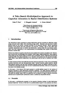
3.4 Investigating the Progress of the Algorithms In the first phase of our experiments the dynamics of the cost function during the search was investigated for both presented algorithms. The algorithms were launched on a series of benchmark datasets while employing the cost function presented by formula (6). In the experiments Nmov = 15 000 000. On the graphs presented in Figures 2-3 the y axis represents the current cost and the x axis represents the number of current move. The current cost is shown in units of 100 000 moves. When the figure is labelled with “TPSA” it is describing the time-predefined simulated annealing approach and when it is labelled “DC” it describes the degraded ceiling algorithm. The behaviour of time-predefined simulated annealing on the KFU-S-93 problem is shown in Figure 2. Following the common practice, we tried different values of T0 and Tf and chose the ones which produced the best results in the shortest time. In our case T0 = 5000 and Tf = 0.05.

10

Figure 2: Progress of time-predefined simulated annealing on KFU-S-93 The progress depicted in Figure2 is typical for simulated annealing. It generally starts with relatively fast improvement of the cost function and then slows until convergence. The fluctuations of the graph show the occasional acceptance of worse solutions. The amplitude of those up-and-down moves is higher at the beginning of the process and degrades to the end of the process (due to reduction of the temperature). However, the reason for the significant fluctuations in the middle of the search is unknown. It does give an impression about the general disorganisation of the process. The convergence is completed somewhere not far from the given number of moves. This means that the value of Tf was chosen almost correctly (but we cannot say anything about T0). It is clear that incorrect setting of the final temperature can lead to either unreasonable idle steps (if Tf is too small), or loss of quality (if Tf too high). The algorithm spends almost half of its processing time very close to the point of convergence and the best solution was produced far before the predefined number of moves. Next we launched the degraded ceiling algorithm on the same problem under the same conditions. The progress of this search is shown in Figure 3.

Figure 3: Progress of the degraded ceiling algorithm This diagram shows how strictly the search follows the linear movement of the ceiling. The fluctuations are seen only in the first half, but later all solutions become quite close to the ceiling and make very small oscillations. When the process reaches a minimum possible value of cost function, it crosses the ceiling and rapidly converges. This behaviour eliminates the situation known as premature

11

convergence, which can happen in non time-predefined algorithms – when the search is terminated too fast and does not reach a high quality solution. The same progress diagrams were also produced for other datasets from Carter’s collection. They are not presented here but can be found on the following web page: http://www.cs.nott.ac.uk/~yxb/dcs. They were quite similar to the presented ones. The over-riding feature is that the behaviour of time-predefined simulated annealing is more erratic than for degraded ceiling. It keeps only the general direction of the progress while its deviations are different with every launch. In contrast, the shape of the progress diagrams of the degraded ceiling algorithm is approximately the same for all launches with all problems.

3.5 Analysis of the Relationship between Time and Cost. A second set of experiments was performed on datasets from Carter’s collection, and again the cost function presented in (6) was employed. For all datasets, both techniques were launched a number of times with different values of Nmov (simulated annealing operated with the same temperatures as in the previous experiments). The final results of those launches were collected into 26 tables (13 datasets x 2 methods), where each table comprises approximately 50 results. All those tables are available on the following web page: http://www.cs.nott.ac.uk/~yxb/dcs. The most typical samples of them (in the form of diagrams) are presented and discussed below. In all following diagrams the y axis represents the final cost and the x axis represents the number of moves taken by the search session. We discuss the results in the context of the number of enrolments for each problem (given in the right-hand column in Table 1), which can be considered as a certain measure of the problem’s size. Firstly, we consider the three “largest” problems: PUR-S-93, UTA-S-92, CAR-S-91. The resulting diagrams are shown in Figures 4-6. For every dataset the given number of timeslots, enrolments and average search speed is indicated.

Figure 4: The diagrams for PUR-S-93 problem (120690 enrolments, 43 timeslots, search speed 82000 moves/sec)

12

Figure 5: The diagrams for UTA-S-92 problem (58981 enrolments, 35 timeslots, search speed 87000 moves/sec)

Figure 6: The diagrams for CAR-S-91 problem (56877 enrolments, 35 timeslots, search speed 73000 moves/sec) The distribution of points in these diagrams obviously confirms the proposition about a clear (and obvious) dependence between the search time and overall solution quality. Even though the results are relatively scattered, there is a clear general tendency to improve the cost function as time increases. Moreover this tendency, for both techniques appears (in almost the same way) for all presented problems. Indeed all three diagrams presented here are surprisingly similar (although, the scale of both axes is individual for each problem). The analysis of the diagrams shows that the slope of the curves is relatively steep on the left hand side of the diagrams (i.e. a small increase in time leads to a high improvement in quality). As the search time gets longer the improvement of solutions becomes slower. Thus, the time-cost diagram of a time-predefined algorithm can be approximated as a monotonically lowered function, which asymptotically approaches some limit. This limit is obviously better than the local optimum (produced by hill-climbing). Possibly it is the minimum for the explored area (which can be separated in the case of a disconnected search space). The particular shape of the time-cost curve depends on the different problem’s characteristics. To investigate the influence of the problem’s size we next consider the diagrams for the “smallest” problems from Carter’s collection: EAR-F-83, YOR-F-83, STA-F-83 (Figures 7-9).

13

Figure 7: The diagrams for EAR-F-83 problem (8108 enrolments, 24 timeslots, search speed 99000 moves/sec)

Figure 8: The diagrams for YOR-F-83 problem (6029 enrolments, 21 timeslots, search speed 44000 moves/sec)

Figure 9: The diagrams for STA-F-83 problem (5751 enrolments, 13 timeslots, search speed 82000 moves/second) These diagrams are clearly different from the ones obtained for the “largest” problems. They show a sharp rise in the final quality with relatively short computational times but further prolongation of the search has very low influence on the result (i.e. the rest of the diagram remains almost flat).

14

Thus the general property of the time-predefined algorithms (i.e. that the longer search produces the better result) holds mostly for the “large” problems while it plays less of a role for the smaller size problems. This is in accordance with what we would expect: the larger problems need more work! With the “middle-sized” problems the presented techniques usually behave in an intermediate way (which is also in accordance with what we would expect). An example of such a dataset (UTE-S-92) is presented on Figure 10.

Figure 10: The diagrams for UTE-S-92 problem (11796 enrolments, 10 timeslots, search speed 203000 moves/sec)

3.6 A Comparison of Time-Predefined Simulated Annealing and Degraded Ceiling with the Current State-of-the-Art. To fully evaluate our techniques, we compare them with recently published results on the same benchmark problems. We consider the results produced by Carter, Laporte and Lee (Carter, Laporte and Lee 1996) by employing several sequencing heuristics with backtracking. We also compare against some very recent results that were produced by Di Gaspero and Shaerf (Di Gaspero and Shaerf 2001). They used tabu search with a variable tabu list. For every dataset Carter published four results, obtained with different heuristics. Di Gaspero and Shaerf presented their best and average values. For comparison purposes we present the best and worst of Carter’s results, the best and average results of Di Gaspero and Shaerf and the best, worst and average results for both of our algorithms. Note that Carter’s results are obtained by using different algorithms whereas Di Gaspero and Shaerf’s results (and our results) employ the same approach. The average values of our results can be estimated while selecting a proper range of samples. The solutions of “short-time” searches (placed in the left hand sides of our diagrams in the previous section) are too poor and are shown mainly for illustration purposes. Therefore, as the search time (at the end of each diagram) is quite acceptable (i.e. we consider its right hand side as within the recommended range). Thus our average values are calculated as an average cost of the five rightmost points on our diagrams. All of the results are summarised in Table 2. Dashes show that the corresponding data was not published. We also include, in the table, a computational time (in seconds) for each best cost. However, this is done only to give a notion about a range of useful time periods because as the published results were produced with different hardware and algorithmic solutions, the search times of the different techniques cannot be sensibly compared.

15

Table 2: Published and our results for proximity cost Carter et al. Data set

Time slots

Gaspero and Shaerf

Cost

best

Time for best worst average (sec)

Time-predefined SA

Cost

best

Time for best (sec) worst average

Degraded ceiling

Cost

best

Time for best (sec) worst average best

Cost

Time for best (sec) worst average

CAR-F-92

32

6.2

7.6

-

47.0

5.2

-

5.6

860.6

4.4

5.1

4.5

295

4.2

5.1

4.3

274

CAR-S-91

35

7.1

7.9

-

20.7

6.2

-

6.5

30.2

5.0

6.3

5.3

256

4.8

6.1

5.0

328

EAR-F-83

24

36.4

46.5

-

24.7

45.7

-

46.7

4.6

35.0

41.1

37.3

589

35.4

41.7

36.7

134

HEC-S-92

18

10.8

15.9

-

7.4

12.4

-

12.6

3.7

10.6

13.2

11.4

1730

10.8

12.4

11.5

278

KFU-S-93

20

14.0

20.8

-

120.2

18.0

-

19.5

12.3

14.2

16.2

14.9

586

13.7

15.6

14.4

729

LSE-F-91

18

10.5

13.1

-

48.0

15.5

-

15.9

20.3

11.0

14.0

12.0

541

10.4

12.6

11.0

1030

PUR-S-93

43

3.9

5.0

-

21729

-

-

-

5.0

6.0

5.1

1395

4.8

6.0

4.9

1412

RYE-S-93

23

7.3

10.0

-

507.2

-

-

-

9.2

10.6

9.6

959

8.9

10.3

9.3

752

STA-F-83

13

161.5

165.7

-

5.7

160.8

-

166.8

3.9

159.0

160.8

159.4

190

159.1

160.3

159.4

157

TRE-S-92

23

9.6

11.0

-

107.4

10.0

-

10.5

16.2

8.6

9.8

8.9

326

8.3

9.6

8.4

392

UTA-S-92

35

3.5

4.5

-

664.3

4.2

4.5

50.7

3.5

4.2

3.6

906

3.4

4.1

3.5

585

UTE-S-92

10

25.8

38.3

-

9.1

29.0

-

31.3

42.4

25.7

30.7

27.2

65

25.7

29.3

26.2

236

YOR-F-83

21

41.7

49.9

-

271.4

41.0

-

42.1

25.2

36.9

40.6

37.5

820

36.7

40.7

37.2

546

16

The figures in the table demonstrate the power of the proposed approaches. Their performance is better (by all quality indices) than Di Gaspero and Shaerf’s tabu search on all the benchmark problems. For eleven of the thirteen problems our algorithms achieved a better cost function value than any of the currently published ones. For five of those problems the best published results are worse than even our average outcome (in a sixth problem they are equal). It is interesting to note that for two of the problems (the largest one and a medium sized one) Carter has an approach, which produces better quality solutions than both of our techniques although, as mentioned above, Carter’s results do not represent one single approach (they employ different heuristics). When comparing the outcomes of our two techniques with each other, it is evident that degraded ceiling performs slightly better than time-predefined simulated annealing. Also, for most of the problems the time-cost diagrams for degraded ceiling are less scattered. Also, in Table 2 it can be seen that degraded ceiling outperforms simulated annealing in 9 cases by the best values and in 11 cases by the average ones. In contrast, simulated annealing is correspondingly better in terms of best values in 3 cases and in terms of average values in just one case. Also, it is only with small-size problems. Note that the two approaches have an equal best value for UTE-S-92 and an equal average value for STA-F-83. Perhaps the timepredefined simulated annealing approach does not perform as well because of poor values of the initial and final temperatures. However, such a situation is characteristic of simulated annealing and the degraded ceiling approach is free of this uncertainty. This alone leads us towards the conclusion that the degraded ceiling algorithm is superior to the time-predefined simulated annealing approach. When this particular advantage is taken together with its superior performance (overall) on the benchmark problems then the evidence of its superiority over time-predefined simulated annealing becomes overwhelming (at least for these benchmark examination timetabling problems).

3.7 Experiments with More Advanced Problems Finally, we evaluated the performance of our approach with more complex problems (in terms of more constraints). Three datasets were chosen where, in addition to the clash-free requirement, the seats constraint (7) is considered as a hard constraint. The distribution of timeslots among days (9) is also taken into account. Hence the cost function is calculated by (12). The characteristics of these problems are presented in Table 3. Table 3: Additional characteristics of problems Data

Seats

Periods

Enrolments

KFU-S-93

1955

21

25,118

NOTT-94

1550

23

33,997

CAR-F-92

2000

36

55,552

In these experiments the simulated annealing parameters were changed to T0 = 1000 and Tf = 0.04) after a series of experiments that suggested that these were good initial values to take. Values of the other parameters were the same as in the previous experiments. The produced time-cost diagrams are presented in Figures11-13.

17

Figure 11: Time-cost diagram for Kfu-s-93 problem (speed 260000 moves/second)

Figure 12: Time-cost diagram for Nott-94 problem (speed 174000 moves/second)

Figure 13: Time-cost diagram for Car-f-92 problem (speed 87000 moves/second)

18

The results obtained by both of our algorithms are compared with the published results obtained by the multi-stage memetic algorithm of (Burke and Newall 1999). There is a series of comparisons in (Burke and Newall 1999) which establish that the multistage memetic algorithm had the best published results on these problems up until the development of the algorithm presented in this paper. In addition, to give a more complete evaluation we also present the tabu search results obtained by Di Gaspero and Shaerf (Di Gaspero and Shaerf 2001) on these 3 problems. In (Burke and Newall 1999) and (Di Gaspero and Shaerf 2001) there is a fourth benchmark problem (PUR-S-93) that is evaluated and discussed. However, the number of timeslots was taken to be 30, which we strongly believe is insufficient for producing a feasible timetable. Both of the approaches in those papers publish results which are infeasible i.e. they generate high values of the cost function because a very high additional value is included when a hard constraint is broken. The problem was intentionally excluded from this comparison because our two approaches consider only feasible solutions. If we cannot find a solution which satisfies the hard constraints then they cannot cope. However the definition of hard constraints is, of course, that they must be satisfied in all cases. The final figures are presented in Table 4.

19

Table 4: Published and our results for weighted sum of adjacent and overnight conflicts Multi-stage memetic algorithm Data set

Time slots

Gaspero and Shaerf

Cost

Time-predefined SA

Cost

best

Time for best worst average (sec)

best

Time for best (sec) worst average

Degraded ceiling

Cost

Cost

best

Time for best (sec) Worst average best

Time for best (sec) worst average

KFU-S-93

21

1388

2662

1626

105

1733

-

1845

n/a

1573

2448

1825

407

1321

2161

1470

345

NOTT-94

23

490

1022

552

467

751

-

810

n/a

522

1015

635

249

384

862

433

612

CAR-F-92

36

1665

4806

1765

186

3048

-

3377

n/a

1951

3622

2250

1220

1506

3536

1610

1268

20

This comparison once more justifies the power of the proposed approach. Indeed, it is clear here that degraded ceiling is far superior to time-predefined simulated annealing. In fact it is far superior (in terms of the quality of its results) to all previously published approaches on these problems. Moreover, the presented time-cost diagrams show the potential for further improvement of results (i.e. there is a clear slope in the right hand side of the diagrams). We did not continue with experiments, which went beyond the right hand side of the diagrams for all 3 problems because of the extreme computational expense. However, the degraded ceiling algorithm was launched on the NOTT-94 problem for extremely long periods to give us some indication of what it could produce with enough computational time (Table 5). Table 5: The best results, obtained for Nott-94 problem by degraded ceiling search Time (hours)

Cost

2.5

256

67

225

As we expected from examining the diagrams, an extremely long search can produce extremely good results. Note that although the solution with a cost of 225 took over 67 hours, we ran it over a weekend (when the machine would otherwise have been idle) and we produced a result which is more than twice as good as the previous best published solution. It is clear that while this ability may not be appreciated by all users, there is a definite potential for incorporating this approach into real world examination timetabling systems (and indeed other scheduling systems).

4. A Brief Note about the Comparison of Time-Predefined Algorithms with other Approaches The comparison of our results with previously published ones, given in Tables 2 and 4 is presented in a traditional way (as it is usually conducted with non time-predefined algorithms). It only expresses a rough idea about the range of the presented values of the cost function. However, a formal comparison (which takes into account both cost and time) of the proposed approach with non time-predefined techniques leads to some problems. When embedding time predefinition into search algorithms it is possible to express their performance as a function: one can get any solution (within some range) as long as one pays the necessary cost in time. On the other hand, the outcome of any non time-predefined technique can be thought as a single time-cost point. We illustrate the relationship between such techniques and a time-predefined approach in Figure 14. The dotted line represents the time-cost trade-off of a time-predefined algorithm A. A solution, produced by a traditional algorithm B (point B) has worse time and cost than A. Thus a preference for algorithm A over B is evident. However, while evaluating the point C (the solution, produced by another non time-predefined algorithm C) we cannot make any general decision about the preference of either algorithm. Algorithm C is clearly preferable to A between points x and y but not necessarily outside these points.

21

Cost

B x C

y

A Time

Figure 14: The example of uncertainty in comparison of the time-cost diagram with the single solution. More uncertainty is connected with the scatter of results. In traditional local search algorithms there is a common practice to run the algorithm several times in order to get the best possible value of the cost function. In contrast, in time-predefined algorithms the aim is to use all the time effectively in a single search for a high quality solution. Also the classical local search algorithms are characterised by the presence of a number of parameters whose values are tuned by performing many experiments. This time should be taken into account when the total time of the solution process is calculated. However, the proposed degraded ceiling algorithm is more free of such parameters and spends almost all of its time only in the search procedure.

5. Conclusions and Future Work Two algorithms where the executional time can be defined in advance were presented. These algorithms between them produced the best published results on all but two benchmark problems. The degraded ceiling algorithm is preferred because it produces most of the best results on these problems (and all of the best results on a further three, more complicated, benchmark problems) in addition to having the feature that its only initial parameter is time although an indication of the desired cost is also required. The experiments and evaluation have provided significant evidence to support the (rather obvious) hypothesis that the quality of solutions can be improved by increasing the search period as long as care is taken in intelligently guiding the search process into (hopefully) fruitful areas of the search space. This allows the User to choose a balance between the quality of a solution and the processing time that suits the user and takes into consideration the nature of the problem, his/her preferences and/or possibilities. A detailed study of possible user strategies while operating with time-predefined algorithms is the subject of future work. It is possible that multiple attribute decision making may yield benefits while considering the quality of solution and computational time as two user objectives. Additionally, some methods suitable for the formal comparison of the time-cost indexes of different algorithms could be defined and investigated. To expand the practical benefits of the presented approaches, it would be worth more accurately investigating their properties, such as the dependence of the time-cost diagram on a problem’s size (and on other characteristics of a problem). Another direction would be to investigate the influence of an initial solution on the overall result while exploring different initialisation methods. Also in our work we did not touch on the question about neighbourhood variation, which probably influences the result as well as questions about disconnected search spaces, relaxation of a problem, kempe or s-chains, etc. The described degraded ceiling algorithm employs a linear reduction of the ceiling as the simplest variant. It seems reasonable to investigate other ways of reducing the ceiling. Also the degraded ceiling algorithm is open to different extensions and hybridisations. Our future work will include investigation of the possibilities of the algorithms to operate with population-based metaheuristics and also for solving

22

multiobjective problems. Also, for certain, the family of time-predefined techniques is not limited to the two proposed methods. We believe that the predefinition of time can indeed be embedded into other techniques.

References APPLEBY, J.S., D. V. BLAKE AND E. A. NEWMAN. 1960. Techniques for Producing School Timetables on a Computer and their Application to Other Scheduling Problems. The Computer Journal 3, 237-245. BOIZUMAULT, P., Y. DELON AND L. PERIDY. 1996. Constraint Logic Programming for Examination Timetabling. Journal of Logic Programming 26(2), 217-233. BOUFFLET, J.P., AND S. NEGRE. 1996. Three Methods Used to Solve an Examination Timetabling Problem. E. Burke, P. Ross, eds. The Practice and Theory of Automated Timetabling: Selected Papers (ICPTAT ‘95). Lecture Notes in Computer Science 1153. Springer-Verlag, Berlin Heidelberg, New York, 327-344. BRELAZ, D. 1979. New Methods to Color the Vertices of a Graph. Communication of the ACM 22(4), 251-256. BULLNHEIMER, B. 1998. An Examination Scheduling Model to Maximize Students’ Study Time. E. Burke, M. Carter, eds. The Practice and Theory of Automated Timetabling: Selected Papers (PATAT ‘97). Lecture Notes in Computer Science 1408. Springer-Verlag, Berlin Heidelberg, New York, 78-91. BURKE, E. K., D. G. ELLIMAN AND R. F. WEARE. 1995a. A Hybrid Genetic Algorithm for Highly Constrained Timetabling Problems. L. J. Eshelman, editor. Genetic Algorithms: Proceedings of the 6th International Conference. San Francisco, Morgan Kaufmann, 605-610. BURKE, E. K., D. G. ELLIMAN AND R. F. WEARE. 1995b. Specialised Recombinative Operators for Timetabling Problems. T. C. Fogarty, editor. AISB Workshop on Evolutionary Computing. Lecture Notes in Computer Science 993. Springer-Verlag, Berlin Heidelberg, New York, 75-85. BURKE, E. K., D. G. ELLIMAN, P. H. FORD AND R. F. WEARE. 1996a. Examination Timetabling in British Universities: a Survey. E. Burke, P. Ross, eds. The Practice and Theory of Automated Timetabling: Selected Papers (ICPTAT ‘95). Lecture Notes in Computer Science 1153. Springer-Verlag, Berlin Heidelberg, New York, 76-90. BURKE, E. K., J. P. NEWALL AND R. F. WEARE. 1996b. A Memetic Algorithm for University Exam Timetabling. E. Burke, P. Ross, eds. The Practice and Theory of Automated Timetabling: Selected Papers (ICPTAT ‘95). Lecture Notes in Computer Science 1153. Springer-Verlag, Berlin Heidelberg, New York, 241-250. BURKE, E. K., J. P. NEWALL AND R. F. WEARE. 1998. Initialization Strategies and Diversity in Evolutionary Timetabling. Evolutionary Computation 6(1), 81-103. BURKE, E. K. AND J. P. NEWALL. 1999. A Multi-Stage Evolutionary Algorithm for the Timetabling Problem. The IEEE Transactions of Evolutionary Computation 3.1, 63-74. BURKE, E. K., Y. BYKOV AND S. PETROVIC. 2001. A Multicriteria Approach to Examination Timetabling. E. Burke, W. Erben, eds. The Practice and Theory of Automated Timetabling III: Selected

23

Papers (PATAT 2000). Lecture Notes in Computer Science 2079. Springer-Verlag, Berlin Heidelberg, New York, 118-131. BURKE, E. K. AND S. PETROVIC. 2002. Recent Research Directions in Automated Timetabling. to appear in European Journal of Operational Research - EJOR. CARTER M.W. 1986. A Survey of Practical Applications of Examination Timetabling Algorithms. Operations Research 34(2),193-201. CARTER, M. W., G. LAPORTE AND J. W. CHINNECK. 1994. A General Examination Scheduling System. Interfaces 24, 109-120. CARTER, M. W. AND G. LAPORTE. 1996. Recent Developments in Practical Examination Timetabling. E. Burke, P. Ross, eds. The Practice and Theory of Automated Timetabling: Selected Papers (ICPTAT ‘95). Lecture Notes in Computer Science 1153. Springer-Verlag, Berlin Heidelberg, New York, 3-21 CARTER, M. W., G. LAPORTE AND S. Y. LEE. 1996. Examination Timetabling: Algorithmic Strategies and Applications. Journal of Operational Research Society 47(3), 373-383. COLE, A. J. 1964. The Preparation of Examination Timetables Using a Small-Store Computer. The Computer Journal 7, 117-121. CORNE, D., H. L. FANG AND C. MELLISH. 1993. “Solving the Module Exam Scheduling Problem with Genetic Algorithms. P. W./H. Chung, G. Lovergrove, M. Ali, eds. Proceedings of the Sixth International Conference in Industrial and Engineering Applications of Artificial Intelligence and Expert Systems. Gordon and Breach Science Publishers, 370-373. CORNE, D., P. ROSS AND H. L. FANG. 1994. Fast Practical Evolutionary Timetabling. T. C. Fogarty, editor. AISB Workshop on Evolutionary Computing. Lecture Notes in Computer Science 865. Springer-Verlag, Berlin Heidelberg, New York, 250-263. CORNE, D. AND P. ROSS. 1996. Peckish Initialisation Strategies for Evolutionary Timetabling. E. Burke, P. Ross, eds. The Practice and Theory of Automated Timetabling: Selected Papers (ICPTAT ‘95). Lecture Notes in Computer Science 1153. Springer-Verlag, Berlin Heidelberg, New York, 227-240. DAVID, P. 1998. A Constraint-Based Approach for Examination Timetabling Using Local Repair Techniques. E. Burke, M. Carter, eds. The Practice and Theory of Automated Timetabling: Selected Papers (PATAT ‘97). Lecture Notes in Computer Science 1408. Springer-Verlag, Berlin Heidelberg, New York, 169-186. DI GASPERO, L. AND A. SCHAERF. 2001. Tabu Search Techniques for Examination Timetabling. E. Burke, W. Erben, eds. The Practice and Theory of Automated Timetabling III: Selected Papers (PATAT 2000). Lecture Notes in Computer Science 2079. Springer-Verlag, Berlin Heidelberg, New York, 104-117. ERBEN, W. 2001. A Grouping Genetic Algorithm for Graph Colouring and Exam Timetabling. E. Burke, W. Erben, eds. The Practice and Theory of Automated Timetabling III: Selected Papers (PATAT 2000). Lecture Notes in Computer Science 2079. Springer-Verlag, Berlin Heidelberg, New York, 132156.

24

ERGUL, A. 1996. GA-Based Examination Scheduling Experience at Middle East Technical University. E. Burke, P. Ross, eds. The Practice and Theory of Automated Timetabling: Selected Papers (ICPTAT ‘95). Lecture Notes in Computer Science 1153. Springer-Verlag, Berlin Heidelberg, New York, 212-226. GLOVER, F. 1986. Future Paths for Integer Programming and Links to Artificial Intelligence. Computers & Operational Research, v5, 533-549. HERTZ, A. 1991. Tabu Search for Large Scale Timetabling Problems. European Journal of Operational Research 54, 39-47. KIRKPATRICK, S., J. C. D. GELLAT AND M. P. VECCI. 1983. Optimization by Simulated Annealing. Science 220, 671-680. MATULA, D. W., G. MARBLE AND I. D. ISAACSON. 1972. Graph Coloring Algorithms. R. C. Read, editor. Graph Theory and Computing. Academic Press, New York, 109-122. PECK, J. E. L. AND M. R. WILLIAMS. 1966. Algorithm 286 - Examination Scheduling. Communication of the ACM 9, 433-434. REEVES C. R. 1996. Modern Heuristic Techniques. Modern Heuristic Search Methods. John Willey & Sons. REIS, L. P., AND E. OLIVEIRA. 2000. Examination Timetabling using Set Variables. Proceedings of the 3rd International Conference on the Practice and Theory of Automated Timetabling PATAT2000, Konstanz, Germany, 181-183. ROSS P. AND D. CORNE. 1995. Comparing Genetic Algorithms, Simulated Annealing and Stochastic Hillclimbing on Timetabling Problems. T. C. Fogarty, editor. AISB Workshop on Evolutionary Computing. Lecture Notes in Computer Science 993. Springer-Verlag, Berlin Heidelberg, New York, 92102. SCHAERF, A. 1999. A Survey of Automated Timetabling. Artificial Intelligent Review 13, 87-127. TERASHIMA-MARIN, H., P. M. ROSS AND M. VALENZUELA-RENDON. 1999. Evolution of Constraint Satisfaction Strategies in Examination Timetabling. Proceedings of the Genetic and Evolutionary Computation Conference (GECCO-99). Morgan Kaufmann, 635-642. THOMPSON, J. M. AND K. A. DOWSLAND. 1996a. General Cooling Schedules for a Simulated Annealing Based Timetabling System. E. Burke, P. Ross, eds. The Practice and Theory of Automated Timetabling: Selected Papers (ICPTAT ‘95). Lecture Notes in Computer Science 1153. Springer-Verlag, Berlin Heidelberg, New York, 345-363. THOMPSON, J. M. AND K. A. DOWSLAND. 1996b Variants of Simulated Annealing for the Examination Timetabling Problem. Annals of Operations Research 63, 105-128. THOMPSON, J. M. AND K. A. DOWSLAND. 1998. A Robust Simulated Annealing Based Examination Timetabling System. Computers and Operational Research 25(7/8), 637-648. WHITE, G. M. AND B. S. XIE. 2001. Examination Timetables and Tabu Search with Longer-Term Memory. E. Burke, W. Erben, eds. The Practice and Theory of Automated Timetabling III: Selected

25

Papers (PATAT 2000). Lecture Notes in Computer Science 2079. Springer-Verlag, Berlin Heidelberg, New York, 85-103. WILLIAMS, M. R. 1974. Heuristic Procedures - (if they Work, Leave Them Alone). Software Practice and Experience 4, , 237-240.

26