The use of Answer Set Programming (ASP) tools to represent temporal scenar- ios for Non-Monotonic Reasoning (NMR) has some important limitations. ASP.
STeLP – a Tool for Temporal Answer Set Programming? Pedro Cabalar and Mart´ın Di´eguez Department of Computer Science, University of Corunna (Spain) {cabalar,martin.dieguez}@udc.es
Abstract. In this paper we present STeLP, a solver for Answer Set Programming with temporal operators. Taking as an input a particular kind of logic program with modal operators (called Splitable Temporal Logic Program), STeLP obtains its set of temporal equilibrium models (a generalisation of stable models for this extended syntax). The obtained set of models is represented in terms of a deterministic B¨ uchi automaton capturing the complete program behaviour. In small examples, this automaton can be graphically displayed in a direct and readable way. The input language provides a set of constructs which allow a simple definition of temporal logic programs, including a special syntax for action domains that can be exploited to simplify the graphical output. STeLP combines the use of a standard ASP solver with a linear temporal logic model checker in order to find all models of the input theory.
1
Introduction
The use of Answer Set Programming (ASP) tools to represent temporal scenarios for Non-Monotonic Reasoning (NMR) has some important limitations. ASP solvers are commonly focused on finite domains and so, representation of time usually involves a finite bound. Typically, variables ranging over transitions or time instants are grounded for a sequence of numbers 0, 1, . . . , n where n is a finite length we must fix beforehand. As a result, for instance, we cannot check the non-existence of a plan for a given planning problem, or that some transition system satisfies a given property for any of its possible executions, or that two representations of the same dynamic scenario are strongly equivalent (that is, they always have the same behaviour for any considered narrative length) to mention three relevant examples. To overcome these limitations, [1] introduced an extension of ASP called Temporal Equilibrium Logic. This formalism combines Equilibrium Logic [2] (a logical characterisation of ASP) with Linear Temporal Logic (LTL) [3] and provides a definition of the temporal equilibrium models (analogous to stable models) for any arbitrary temporal theory. ?
This research was partially supported by Spanish MEC project TIN2009-14562-C0504 and Xunta de Galicia project INCITE08-PXIB105159PR.
In this paper we introduce STeLP, a system for computing the temporal equilibrium models of a particular class of temporal theories called Splitable Temporal Logic Programs (STLP). This class suffices to cover most frequent examples in ASP for dynamic domains. More importantly, the temporal equilibrium models of an STLP have been shown to be computable in terms of a regular LTL theory (see the companion paper [4]). This feature is exploited by STeLP to call an LTL model checker as a backend.
2
Splitable Temporal Logic Programs
Temporal Equilibrium Logic (TEL) shares the syntax of propositional LTL, that is, propositional formulas plus the unary temporal operators1 � (read as “always”), ♦ (“eventually”) and (“next”). TEL is defined in two steps: first, we define the monotonic logic of Temporal Here-and-There (THT); and second, we select TEL models as some kind of minimal THT-models obtaining nonmonotonicity. For further details, see [5]. Definition 1 (STLP). An initial rule is an expression of one of the forms: A1 ∧ · · · ∧ An ∧ ¬An+1 ∧ · · · ∧ ¬Am → Am+1 ∨ · · · ∨ As
(1)
B1 ∧ · · · ∧ Bn ∧ ¬Bn+1 ∧ · · · ∧ ¬Bm → Am+1 ∨ · · · ∨ As
(2)
where Ai are atoms and each Bj can be an atom p or the formula p. A dynamic rule has the form �r where r is an initial rule. An Splitable Temporal Logic Program (STLP) Π is a set of (initial and dynamic) rules. � The body (resp. head ) of a rule is the antecedent (resp. consequent) of its implication connective. The following theory Π1 is an STLP: ¬a ∧ b → a
�(a → b)
�(¬b → a)
In [4] it is shown how the temporal equilibrium models of an STLP Π correspond to the LTL models of Π ∪LF (Π) where LF (Π) are loop formulas adapted from the result in [6]. For further details and a precise definition, see [4].
3
The input language
The input programs of STeLP adopt the standard ASP notation for conjunction, negation and implication, so that, an initial rule like (1) is represented as: Am+1 v . . . v As :- A1 , . . . ,An , not An+1 , . . . , not Am Temporal expressions are represented following the correspondences: 1
As shown in [5], the LTL binary operators U (“until”) and R (“release”) can be removed by introducing auxiliary atoms.
α − 7 → o α �(α → β) − 7 → β::- α
�α − 7 → always α α U β 7−→ α until β
Operators always and until can only be used for constraints (that is, rules with empty head). In fact, this is because STeLP allows a more general type of constraints than those defined in splitable form, since we can specify any arbitrary combination of propositional connectives with {o, always, until} as a body of any constraint (initial or dynamic). As an example of the STeLP input syntax, Π1 would be represented as: o a :- not a, o b.
b ::- a.
o a ::- not b.
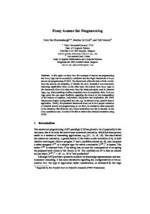
In STeLP we can also use rules where atoms have variable arguments like p(X1 ,. . . ,Xn ) and, as happens with most ASP solvers, these are understood as abbreviations of all their ground instances. A kind of safety condition is defined for variables occurring in a rule. To this aim, notice that using any dynamic predicate for that purpose is not directly possible, since their truth may infinitely vary along time. Thus, we will previously distinguish a family of predicates that satisfy the property �( p(X) ↔ p(X) ) for any tuple of elements X. That is, these predicates maintain a fixed truth value along time, and so, they will be called static. STeLP allows declaring static operators with a list of pairs name/arity preceded by the keyword static. As expected, all built-in relational operators =, !=, , = are implicitly defined as static predicates with their usual meaning. An initial or dynamic rule is safe when: 1. Any variable X occurring in a rule B → H or �(B → H) occurs in some positive literal in B for some static predicate p. 2. Initial rules of the form B → H where at least one static predicate occurs in the head H only contain static predicates (these are called static rules). All rules in an STeLP program must be safe. Since static predicates must occur in any rule, STeLP allows defining global variable names with a fixed domain, in a similar way to the lparse2 directive #domain. For instance, the declaration domain switch(X), opp(V,W). means that any rule referring to variable X is implicitly extended by including an atom switch(X) in its body, whereas any rule containing V or W (or both) is extended with a body atom opp(V,W). All predicates used in a domain declaration must be static – as a result, they will be implicitly declared as static, if not done elsewhere. As an example, consider the classical puzzle where we have a wolf w, a sheep s and a cabbage c at one bank of a river. We have to cross the river carrying at most one object at a time. The wolf eats the sheep, and the sheep eats the cabbage, if no people around. Action m(X) means that we move some item w,s,c from one bank to the other. We assume that the boat is always switching its bank from one state to the other, so when no action is executed, this means we moved the boat without carrying anything. We will use a unique fluent at(Y,B) meaning that Y is at bank B being Y an item or the boat b. The complete encoding is shown in Figure 3. 2
http://www.tcs.hut.fi/Software/smodels/lparse.ps.gz
% Domain predicates domain item(X), object(Y), opp(A,B). opp(l,r). opp(r,l). item(w). item(s). item(c). object(Z) :- item(Z). object(b). o at(X,A) ::- at(X,B), m(X). % Effect axiom for moving o at(b,A) ::- at(b,B). % The boat is always moving ::- m(X), at(b,A), at(X,B). % Action executability ::- at(Y,A), at(Y,B). % Unique value constraint o at(Y,A) ::- at(Y,A), not o at(Y,B). % Inertia ::- at(w,A), at(s,A), at(b,B). % Wolf eats sheep ::- at(s,A), at(c,A), at(b,B). % Sheep eats cabbage a(X) ::- not m(X). % Choice rules for action m(X) ::- not a(X). % execution ::- m(X), item(Z), m(Z), X!=Z. % Non-concurrent actions at(Y,l). % Initial state g ::- at(w,r), at(s,r), at(c,r). % Goal predicate :- always not g. % Goal must be satisfied Fig. 1. Wolf-sheep-cabbage puzzle in STeLP.
A feature that causes a difficult reading of the obtained automaton for a given STLP is that all the information is represented by formulas that occur as transition labels, whereas states are just given a meaningless name. As opposed to this, in an actions scenario, one would expect that states displayed the fluents information and transitions only contained the actions execution. To make the automaton closer to this more natural representation, we can distinguish predicates representing actions and fluents. For instance, in the previous example, we would further declare: action m/1. fluent at/2. STeLP uses this information so that when all the outgoing transitions from a given state share the same information for fluents, this is information is shown altogether inside the state, and removed from the arc labels. Besides, any symbol that is not an action or a fluent is not displayed (they are considered as auxiliary). As a result of these simplifications, we may obtain several transitions with the same label: if so, they are collapsed into a single one.
4
Implementation
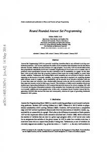
STeLP is a Prolog application that interacts with the standard ASP solver DLV3 and the LTL model checker SPOT4 . As shown in Figure 2, it is structured in several modules we describe next. In a first step, STeLP parses the input program, detecting static and domain predicates, checking safety of all rules, and separating the static rules. It also appends static predicates to rule bodies for all variables with global domain. The 3 4
http://www.dbai.tuwien.ac.at/proj/dlv/ http://spot.lip6.fr/
Fig. 2. Structure of STeLP system.
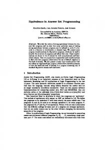
set of static rules is fed to DLV to generate some model (among possible) that will provide the extension for all static predicates. The number of static models that STeLP will consider is given as a command line argument. Each static model will generate a different ground program and a different automaton. Once a static model is fixed, STeLP grounds the non-static rules input program. Each ground instance is evaluated and, if the body of the ground rule becomes false, the rule is deleted. Otherwise all static predicates of the rule are deleted from its body. The next step consists in computing the loop formulas for the ground STLP we have obtained. This implies obtaining a dependency graph and computing its strongly connected components (the loops) using Tarjan’s algorithm [7]. The STLP together with its loop formulas is then used as input for the LTL solver SPOT, which returns a deterministic B¨ uchi automaton. In a final step, STeLP parses and, if actions and fluents are defined, simplifies the automaton as described before. The tool Graphviz5 is used for generating a graphical representation. For instance, our wolf-sheep-cabbage example throws the diagram in Figure 3 where we can actually see all the accessible states (any movement is reversible) from the initial situation, including the goal situation. As an example of non-existence of plan, if we include the rule ::- at(w,r), at(c,r), at(b,l) meaning that we cannot leave the wolf and the cabbage alone in the right bank, then the problem becomes unsolvable (we get a B¨ uchi automaton with no accepting path). 5
http://www.graphviz.org/
at(b,r),at(c,l) at(s,r),at(w,r)
at(b,l),at(c,l) at(s,l),at(w,r)
m(s)
m(w)
m(c)
m(c)
at(b,l),at(c,l) at(s,r),at(w,l)
at(b,r),at(c,r) at(s,r),at(w,l)
m(s)
at(b,l),at(c,r) at(s,l),at(w,l)
m(w)
∅
at(b,r),at(c,r) at(s,l),at(w,r)
∅
m(s)
at(b,r),at(c,l) at(s,r),at(w,l)
at(b,l),at(c,l) at(s,l),at(w,l)
at(b,r),at(c,r) at(s,r),at(w,r)
init
goal
m(s)
at(b,l),at(c,r) at(s,l),at(w,r)
Fig. 3. Automaton for the wolf-sheep-cabbage example.
References 1. Cabalar, P., Vega, G.P.: Temporal equilibrium logic: a first approach. In: Proc. of the 11th International Conference on Computer Aided Systems Theory, (EUROCAST’07). LNCS (4739). (2007) 241–248 2. Pearce, D.: A new logical characterisation of stable models and answer sets. In: Non monotonic extensions of logic programming. Proc. NMELP’96. (LNAI 1216). Springer-Verlag (1996) 3. Manna, Z., Pnueli, A.: The Temporal Logic of Reactive and Concurrent Systems: Specification. Springer-Verlag (1991) 4. Aguado, F., Cabalar, P., P´erez, G., Vidal, C.: Loop formulas for splitable temporal logic programs (2011) (unpublished draft) http://www.dc.fi.udc.es/~cabalar/lfstlp.pdf. 5. Cabalar, P.: A normal form for linear temporal equilibrium logic. In: Proc. of the 12th European Conference on Logics in Artificial Intelligence (JELIA’10). Lecture Notes in Computer Science. Volume 2258. Springer-Verlag (2010) 64–76 6. Ferraris, P., Lee, J., Lifschitz, V.: A generalization of the Lin-Zhao theorem. Annals of Mathematics and Artificial Intelligence 47 (2006) 79–101 7. Tarjan, R.: Depth-first search and linear graph algorithms. SIAM Journal on Computing 1(2) (1972) 146–160