This paper presents an efficient phase preserving processor for the TOPS (Terrain Observation by Progressive Scans) imaging mode. TOPS has been proposed ...
A TOPSAR Processing Algorithm Based on Extended Chirp Scaling: Evaluation with TerraSAR-X Data. Pau Prats, Adriano Meta, Rolf Scheiber, Josef Mittermayer and Alberto Moreira German Aerospace Center (DLR), Germany Jesús Sanz-Marcos Cota Cero Arquitectura y Algorítmica S.L., Spain
Abstract This paper presents an efficient phase preserving processor for the TOPS (Terrain Observation by Progressive Scans) imaging mode. TOPS has been proposed as a new wide swath imaging mode, which solves the problems of scalloping and azimuth-varying ambiguities introduced by the conventional ScanSAR mode by means of steering the antenna along the azimuth direction. The TOPS signal includes particularities of both ScanSAR and Spotlights modes, but existing processing algorithms do not provide an efficient processing of TOPS data. This paper presents an algorithm based on Extended Chirp Scaling (ECS) together with a new azimuth scaling step. The proposed solution allows also the selection of the final azimuth image sampling without the need of interpolations, hence easing the forthcoming mosaicking of the different subswaths. Real data acquired by TerraSAR-X are used to validate the processor.
1 Introduction Large swath coverage is an essential requirement for several applications. The standard ScanSAR mode achieves this requirement by periodically switching the antenna elevation beam to point at different range subswaths [1], hence acquiring a certain number of bursts per subswath. The trade-off is the azimuth resolution loss due to the reduction of the observation time of targets. However, the ScanSAR mode has some disadvantages besides resolution loss: scalloping (periodical modulation of the amplitude in the focused image), and azimuth-varying ambiguity ratio and noise equivalent sigma-zero (σ 0 ). They are a consequence of the fact that different targets are observed under different portions of the azimuth antenna pattern. In order to reduce these effects, either different bursts are incoherently averaged, with the consequent further reduction of the azimuth resolution, or the antenna pattern is corrected. The latter might result insufficient in scenarios with low singal-to-noise ratio (SNR), since the antenna pattern compensation increases the noise level at burst edges. TOPS (Terrain Observation by Progressive Scans) has been proposed as a new wide swath imaging mode [2]. It overcomes the problems of scalloping and azimuth-varying ambiguities introduced by the conventional ScanSAR mode by means of steering the antenna in the along-track direction. To achieve the same swath coverage and avoid the undesired effects of ScanSAR the antenna is rotated throughout the acquisition from backward to forward at a constant rotation speed ω r (see Figure 1), opposite to the Spotlight case, resulting in the opposite ef-
fect, i.e. a reduction of the azimuth resolution. In this way, all targets are observed by the same azimuth antenna pattern, and therefore the scalloping effect disappears and azimuth ambiguities and signal-to-noise ratio become constant in azimuth. At the end of the burst, the antenna look angle is changed to illuminate a second subswath, pointing again backwards. When the last subswath is imaged, the antenna points back to the first subswath, so that no gaps are left between bursts of the same subswath.
Figure 1: Acquisition geometry of the TOPS imaging mode. Standard processing approaches for other imaging modes (Stripmap, Spotlight, ScanSAR) are not valid for the TOPS mode. Only with pre- and post-processing approaches these algorithms can be used with data acquired in the TOPS mode, with the consequent increase in the computation burden. A dedicated processor must be developed if efficient focusing is desired. Section 2 first analyzes the TOPS signal characteristics. The proposed processor is ex-
pounded in Section 2.2, while Section 3 shows processing results with real data acquired by the TerraSAR-X (TSX) satellite. Finally, Section 4 presents the conclusions.
for each sub-aperture is continued with the corresponding Doppler centroid. To prevent a poor processing result due to the block processing, the sub-apertures are formed with some overlap, e.g. 5%.
2 TOPS Processing 2.1 TOPS signal characteristics The TOPS raw data signal in one burst has similarities with both ScanSAR and Spotlight signals. The TOPS signal resembles the Spotlight signal in the sense that the scene bandwidth is larger than the pulse repetition frequency (PRF). Also, it has similarities with the ScanSAR mode in the sense that the burst duration is shorter than the output focused burst. The signal properties can be clearly visualized by means of a time-frequency diagram. Figure 2 shows the Doppler history of three targets at the same range position (thick solid lines), but at different azimuth positions. The axis of abscissas corresponds to the azimuth time and the axis of ordinates to the instantaneous frequency. The target at the beginning of the burst is observed under a negative squint angle, hence resulting in negative Doppler frequencies. On the other hand, the target at the end of the burst has positive Doppler frequencies. Usually, the total scene bandwidth spans over several PRF intervals, similar as it occurs in the Spotlight mode. Consequently, some procedure is necessary to account for this insufficient sampling of the azimuth signal. Concerning the similarities with ScanSAR, consider the third target depicted in Figure 2. Although it is observed by the middle of the beam at the time instant tc (i.e. beam-center time), after the focusing the target should appear at its zero-Doppler position t0 . Hence, the output focused burst is larger than the burst duration. Figure 2 also considers a possible mean Doppler centroid during the data take given by fc .
Figure 3: Block diagram of the proposed TOPS processor. The steps of RCMC, secondary range compression (SRC) and range compression are carried out using the standard phase functions of ECS [4] (functions H1 , H2 and H3 ) for each sub-aperture. Once in the range-Doppler domain, a novel azimuth scaling is performed, named baseband azimuth scaling, which consists of the phase functions H4 , H5 , H6 and H7 . The first step is the removal of the hyperbolic azimuth phase and its replacement with a purely quadratic phase shape using � � 4π H4 (fa , r) = exp j r · (β(fa ) − 1) λ � � π 2 · exp −j f , (1) Kscl (r) a with β(fa ) =
Figure 2: Time-frequency diagram in the TOPS imaging mode.
2.2 Proposed Processing based on ECS The block diagram of the proposed processor appears in Figure 3. In order to accommodate the larger scene bandwidth, the data are divided in azimuth blocks (subapertures), similarly as done for Spotlight processing in [5]. After the division into sub-apertures, the processing
s
1−
�
λfa 2v
�2
.
(2)
The quadratic phase history is described by the scaling Doppler rate Kscl (r), which depends on range as described in equations (3) to (5): Kscl = −
2v 2 λrscl (r)
rscl0 rrot (r) rrot0 rrot0 − r rrot (r) = , 1 − rscl0 /rrot0 rscl (r) =
(3) (4) (5)
where rscl0 is a scaling range selected according to the desired azimuth image sampling, and rrot0 is the vector distance to the rotation center, which is located behind the
sensor in the TOPS mode. The reason to use this rangedependent scaling range is explained in [3]. Since H4 provokes a shift of the azimuth signals that are not located at the scaling range rscl0 , a slight extension of the azimuth dimension is required. In the next step of the process, an azimuth IFFT is used for a transformation back to the azimuth/range-time, where the individual subapertures are assembled. However, the bandwidth of the signal still exceeds the PRF. Therefore a demodulation can be carried out similar as in [2] by using the following derotation function h i 2 H5 (t, r) = exp −jπKrot (r) · (t − tmid ) , (6)
However, it is also interesting to choose the same azimuth sampling for all subswaths in order to ease their recombination afterwards (no interpolations needed). Therefore, the solution is to find the azimuth sampling that minimizes the needed extension in all subswaths. This can be easily done by plotting the individual extension for every subswath as a function of the azimuth sampling, as exemplified in Figure 4 for a TSX case. The scaling range rrscl0 for every subswath is finally computed using (11).
where tmid is the scene center time. Note that this phase function can also be performed prior to the sub-aperture recombination, as it is applied in the azimuth/range-time domain. The chirp rate used in the de-rotation function depends on range and is given by Krot (r) = −
2v 2 . λrrot (r)
(7)
At this point, the effective chirp rate of the signal is Keff (r) = Kscl (r) − Krot (r). Due to the fact that now the data spectrum for all targets is basebanded, matched filtering can be applied using � � π 2 H6 (fa , r) = W (fa ) · exp j f . (8) Keff (r) a
Figure 4: Selection of the final azimuth sampling. The dashed and solid lines indicate the needed extension for near and far range in a given subswath, respectively.
Note that azimuth sidelobe suppression can be also performed by means of a weighting function W (fa ). An inverse FFT results in a focused signal. However, for phase preserving processing the data must be multiplied by the following phase function " # � �2 rscl0 2 H7 (t, r) = exp jπKt (r) · 1 − · (t − tmid ) , rrot0 (9) where 2v 2 Kt (r) = − . (10) λ · (rrot (r) − rscl (r))
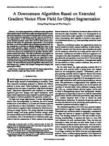
The proposed processor was already validated in [3] by means of simulated point targets and airborne data. Real data acquired by TSX in TOPS mode is presented next. The antenna array of TSX and its flexibility concerning the operational commanding have allowed an efficient implementation of the TOPS mode, even though this mode was not foreseen when designing the system. A data take over Barcelona, Spain, was acquired the 28th of December 2007 in a descending orbit configuration. The TOPS acquisition consists of four subswaths, with a commanded resolution of 16m. The azimuth image sampling that minimizes the extension considering all subswaths is 9m, as shown in Figure 4. Figure 5 shows the focused image, with scene dimensions of 62.3km×90.7km (slantrange×azimuth). There are a total of 6 bursts per subswath and the absence of scalloping is evident. Figure 6 shows a zoom over one of the corner reflectors (CR). Its contour plot can be seen in Figure 7 together with the 3D representation of the impulse response function (IRF). The analyzed values of interest are shown in Table 1, where it should be noted that no weighting for side-lobe suppression was applied, nor the azimuth antenna pattern was corrected. The higher side-lobes in range are due to the fact that no replica was used during the focusing, but the nominal chirp. The phase preservation of the processor has already been proved in [3, 6].
The final image sampling in the azimuth dimension is then given by ∆xfinal = ∆xorig · (1 − rscl0 /rrot0 ) ,
(11)
where ∆xorig is the sampling of the raw data, and rscl0 is selected according to the desired final azimuth image sampling.
2.3 Selection of the Scaling Range Although the proposed approach allows selecting an arbitrary azimuth sampling by means of a proper rscl0 , one must consider that the further away this rscl0 from the subswath range is, the greater the needed extension will be.
3 Image Processing
baseband azimuth scaling also allows selecting the final azimuth image sampling, which is useful since it avoids the need for interpolations to recombine different subswaths. Consequently, the overall focusing is carried out just using FFTs and complex multiplications. For a detailed comparison between ScanSAR and TOPS acquisition modes please refer to [7].
Figure 7: Interpolated (left) contour plot and (right) 3D representation of the IRF of the CR.
Figure 5: TOPS image over Barcelona, Spain.
Table 1: Obtained IRF values for the CR Range PLSR −11.15 dB/−17.33 dB Range ISLR −9.10 dB Measured range resolution 1.33 m Theoretical range resolution 1.33 m Azimuth PLSR −17.32 dB/−16.33 dB Azimuth ISLR −13.32 dB Measured azimuth resolution 14.70 m Theoretical azimuth resolution 14.85 m
Acknowledgments This work has been partially funded by ESA under contract C20679/07/NL/CB.
References [1] K. Tomiyasu: Conceptual Performance of a Satellite Borne, Wide Swath Synthetic Aperture Radar, IEEE Trans. Geosci. Remote Sensing, 19, 1981. [2] F. De Zan et al.: TOPSAR: Terrain Observation by Progressive Scans, IEEE Trans. Geosci. Remote Sensing, 44 (9), Sep. 2006.
Figure 6: Zoom of Figure 5 over the CR, indicated by the red circle.
4 Conclusion A phase preserving TOPS processor has been presented and validated with TSX data. It divides the raw data in azimuth sub-apertures to accommodate the scene bandwidth, while for the azimuth processing a new azimuth scaling approach allows an efficient focusing of the data. The
[3] P. Prats et al.: A SAR Processing Algorithm for TOPS Imaging Mode Based on Extended Chirp Scaling, Proc. IGARSS, Jul. 2007. [4] A. Moreira et al.: Extended Chirp Scaling Algorithm for Air- and Spaceborne SAR Data Processing in Stripmap and ScanSAR Imaging Modes, IEEE Trans. Geosci. Remote Sensing, 34 (5), Sep. 1996. [5] J. Mittermayer et al.: Spotlight SAR Data Processing Using the Frequency Scaling Algorithm, IEEE Trans. Geosci. Remote Sensing, 37 (5), Sep. 1999. [6] A. Meta et al.: First TOPSAR Image and Interferometry Results with TerraSAR-X, Proc. FRINGE, Nov. 2007. [7] A. Meta et al.: TerraSAR-X TOPSAR and ScanSAR Comparison, Proc. IGARSS, Jul. 2008.