IEEE TRANSACTIONS ON CONTROL SYSTEMS TECHNOLOGY, VOL. 20, NO. 4, JULY 2012
1025
A Trajectory Generation Algorithm for Optimal Consumption in Electromagnetic Actuators Antonio Fabbrini, Andrea Garulli, and Paolo Mercorelli
Abstract—Camless internal combustion engines offer improvements over traditional engines in terms of torque performance, reduction of emissions, reduction of pumping losses and fuel economy. Theoretically, electromagnetic valve actuators offer the highest potentials for improving efficiency due to their control flexibility. For real applications, however, the valve actuators developed so far suffer from high power consumption and other control problems. One key point is the design of the reference trajectory to be tracked by the closed loop controller. In this brief, a design technique aimed at minimizing power consumption is proposed. A constrained optimization problem is formulated and its solution is approximated by exploiting local flatness and physical properties of the system. The performance of the designed trajectory is validated via an industrial simulator of the valve actuator. Index Terms—Cost function, electromagnetic devices, motion control, optimization, trajectory design.
I. INTRODUCTION
T
HANKS to the recent rapid progresses in permanent-magnet technology, especially through the use of high-energy-density rare-earth materials, very compact and high-performance electromagnetic actuators are now available. They open new possibilities for high-force motion control in mechatronic applications where a great deal of flexibility, high control dynamics and precise positioning are required at the same time. In the last few years, variable engine valve control has attracted a lot of attention because of its ability to reduce pumping losses (work required to draw air into the cylinder under part-load operation) and to increase torque performance over a wider rage than conventional spark-ignition engine. Variable valve timing also allows control of internal exhaust gas recirculation, thus improving fuel economy and reducing NOx emissions. Besides mechanical and hydraulic variable valve train options, electromagnetic valve actuators have been considered in the literature [1], [2]. Prototype systems have been proposed by several companies in the automotive industry, including FEV Motorentechnik [3], [4], BMW [5], [6], GM [7], Manuscript received August 04, 2010; revised March 10, 2011; accepted May 04, 2011. Manuscript received in final form June 01, 2011. Date of publication June 30, 2011; date of current version May 22, 2012. Recommended by Associate Editor J. Lu. This work was supported by European Commission through Erasmus Project and was technically supported by Institute for Automation and Informatics (IAI), Wernigerode, Germany. A. Fabbrini and A. Garulli are with the Department of Information Engineering, University of Siena, 53100 Siena, Italy (e-mail:
[email protected]). P. Mercorelli is with the Faculty of Automotive Engineering, Ostfalia University of Applied Sciences, 38440 Wolfsburg, Germany (e-mail:
[email protected]). Color versions of one or more of the figures in this brief are available online at http://ieeexplore.ieee.org. Digital Object Identifier 10.1109/TCST.2011.2159006
[8], Renault [1], [9], Siemens [10], and Aura [11]. Recently, a new type of an electromagnetic valve drive system has been proposed and described in [12]. This system incorporates a disk cam with a very desirable non linear profile which functions as a nonlinear mechanical transformer. Recent works testify several technical progresses also in the area of control of electromechanical and electromagnetic drives [13]–[16]. Theoretically, electromagnetic valve actuators offer the highest potential for improving fuel economy due to their control flexibility. In particular they are able to control the superposition of intake and exhaust trajectories in variable way, in order to improve the combustion phases of the motor. In fact, it is known that by mixing exhaust gas with intake air fuel mixture in the cylinder, the internal combustion engine is improved. Fig. 1 shows the considered system along with the related cylinder phase diagram. In particular, Fig. 1(a) shows the intake and exhaust valves together with the cylinders configuration. In Fig. 1(b), the phase diagram of the positions of the intake and exhaust valves is sketched. Two position profiles for each cylinder are represented: one for the intake and the other for the exhaust valve which operate in each cylinder. It is to notice how a crossing point between the closing trajectory of the exhaust and the opening trajectory of the intake is present in every cylinder, in order to guarantee a mix between combusted gas and the new air and gasoline. For real applications, however, the electromagnetic valve actuators developed so far, suffer from high power consumption and other control problems. One key point to reduce the power consumption is the design of an optimal reference trajectory to be tracked by a closed-loop controller. In [17], a technique for the generation of an optimal trajectory is developed by formulating a two-point boundary value optimization problem, and by considering a suitable parametrization of the input voltage. The considered problem is very hardly solvable even by numerical integration methods. In fact, the solution is an optimizing voltage over an input functional space. In this brief, trajectory design is still formulated as a twopoint boundary value optimization problem that explicitly considers the structural physical constraints and the properties of the system. The optimal design problem is then decomposed into three subproblems, corresponding to different branches of the trajectory to be designed. Two subproblems are solved by exploiting flatness, while a linear quadratic regulator (LQR) technique is applied to the subproblem in which the flatness property does not hold. An advantage of the proposed approach is that no numerical integration is required to solve the resulting optimization subproblems. The designed trajectory is validated by using an accurate simulator of the actuator [18], in which tracking of the reference trajectory is performed via cascaded PD controllers combined with a feed-forward regulator. More
1063-6536/$26.00 © 2011 IEEE
1026
IEEE TRANSACTIONS ON CONTROL SYSTEMS TECHNOLOGY, VOL. 20, NO. 4, JULY 2012
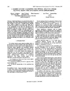
Fig. 2. (a) Detail of the cylinder and cross-section view of the actuator; (b) combined physical characteristics of the intake and exhaust valve of adjacent cylinders for different current values.
Fig. 1. (a) Four-cylinder motor with electromagnetic valves; (b) position phase diagram of the opening and closing valves.
advanced control strategies can be employed, like MPC (see [19] and [20]). A preliminary version of this brief appeared in [21]. This brief is organized in the following way. Section II introduces the dynamic model of the considered actuator and its structural properties. The notion of flatness in nonlinear systems is briefly recalled in Section III. Section IV addresses the reference trajectory design problem and presents the proposed solution. Simulations results are shown in Section V, while conclusions and future perspectives are reported in Section VI. II. DYNAMIC MODEL OF THE INTAKE VALVE ACTUATOR Fig. 2(a) shows the operation principle of the engine valves to be controlled. The intake valve allows air and fuel to rush into the cylinder so combustion can take place. The exhaust valve releases the spent fuel and air mixture from the cylinder. Clearly, the timing of the valve opening and closing strongly influences
the engine efficiency and fuel economy. The optimal choice of the opening and closing timing depends on the simultaneous operation conditions of the engine. In conventional spark-ignition engines the valves are driven by the camshaft and their timing is fixed by the engine speed. The use of electromagnetic valve actuators decouples the valve timing from the engine speed and ensures fully timing variability. If a frequency of around 6000 rpm (revolutions per minute) is considered and a distance of 8 mm must be covered, then a time interval of about 4 ms for opening and closing of the valve is required. This is one of the worst practical cases in which high accelerations up to 4000 m/s have to be achieved, even in case of large disturbances due to the strong cylinder gas force acting against the exhaust valve opening. On the other hand, the power consumption of the device must not exceed a certain threshold. In particular, since the magnetic properties of the ferromagnetic materials are guaranteed for temperature lower than 160 C, electrical power consumption less than 50 W is mandatory. Most electromechanical valve actuators studied so far exploit Maxwell attracting forces at both ends of the motion range [17], [22], [23]. This operation principle is simple to implement, but difficult to control as it is not possible to influence the valve motion in the middle range. Thus,
IEEE TRANSACTIONS ON CONTROL SYSTEMS TECHNOLOGY, VOL. 20, NO. 4, JULY 2012
variable opening strokes, which have recently proven to be efficient for engine operation, are hardly possible. For this reason, attention has been focused on linear motors as valve actuators in order to be able to control the motion across the complete range, including positioning the valve at every specified stroke [24], [25]. In [26] a combination of a linear motor and a reluctance motor was presented. In order to achieve a more compact structure and bigger resulting torque, a rotational geometry of the actuator based on the same principle was presented in [18]. Fig. 2(b) shows the torque characteristics and it is possible to see that controllability of the motor is lost for some values of the angular position. Nevertheless, the compact structure of the valve and its relatively large torque at the start point (valve closed) make this structure very attractive. The considered electromagnetic actuator can be modeled as follows: (1) (2) (3) Equation (1) represents the electrical part of the actuator, where is the coil resistance and the coil inductivity, (2) and (3) describe the mechanical behavior of the actuator, and denotes the inertia moment of the rotor. The state variables are the coil current , the rotor angular position and its angular velocity (hereafter, explicit dependence on time will be omitted unless necessary). In (1), is the input voltage and represents the induced electromagnetic voltage, where is the angular position of the stator poles. In (3), the expression
1027
forces a torque is obtained, which is a nonlinear function of the angular position . III. SYSTEM FLATNESS Before proceeding with the formulation of the trajectory design problem, let us recall the concept of flatness in nonlinear systems, see, e.g., [27]. Roughly speaking, a system is differentially flat if it is possible to find a set of outputs, equal in number to the number of inputs, such that all states and inputs are expressed in terms of those outputs and their derivatives. In other words, if the , and outsystem has state variables , inputs , then the system is flat if it is possible to express puts the state and inputs as (7) for some integer . Differentially flat systems are especially interesting in situations where explicit trajectory tracking is required [28], [29]. Since the behavior of the flat system is given by the flat output, it is possible to plan trajectories in output space, and then map these to the appropriate inputs. System (1)–(3) is not globally flat. In fact, if the angular position of the moving part of the actuator is chosen as the “flat output”, then (8) (9) To check the flatness property, current must be expressed as function of and its derivatives. From (3) and (6), one has (10)
(4) describes the torque generated by the actuator, where (5) (6) are physical constants. Furthermore, is the inertia and moment of the moving part of the actuator-valve system, represents the friction moment in which is the “initial moment” (for ), and is the viscous damping coefficient. is a known function of the angular position which models the spring moment and the magnetic spring moment. In fact, the system consists of two springs, a mechanical and a magnetic one. The mechanical spring is used to guarantee that the valve can remain closed without using electrical energy. The magnetic spring is installed on the driveshaft in order to sustain the electric motor at those angles where the torque produced is too low, in order to reduce the power consumption of the actuator. The magnetic spring is composed by a stator and a rotor both with alternated permanent magnetic poles. From their attractive and repulsive magnetic
It is easy to see that current is not always defined, and thus the flatness conditions are not globally satisfied. In fact, the current presents a singularity whenever is equal to zero, i.e., for . Finally, the input can be expressed in terms of and its derivatives, by substituting (8)–(10) into (1). IV. REFERENCE TRAJECTORY DESIGN The main goal of the control system is to move the valve from the fully-closed to the fully-opened position (and vice versa) avoiding noisy and wearing hits against the hard mechanical stops. The designed trajectory has to satisfy the following several requirements. 1) The trajectory must guarantee that the valve opens and closes with a “soft landing” behavior. 2) Control voltages resulting from the trajectory must be sufficiently far from the maximum voltage thus avoiding wind-up phenomenon which normally destroys system robustness achievable with closed-loop control. 3) The trajectory should optimize the consumption of the electrical and friction energy in order to guarantee the functioning temperature constraints.
1028
IEEE TRANSACTIONS ON CONTROL SYSTEMS TECHNOLOGY, VOL. 20, NO. 4, JULY 2012
B. Proposed Method To solve the optimization problem addressed in the previous section, flatness of the system is exploited. Given the flat output , using (7), it is possible to write the cost function and the constraints as a function of the flat output and its derivatives. In practice, the problem of finding a state trajectory is transformed to the flat space, so that a solution is feasible in the state space if and only if it is feasible in the flat space. The advantage of moving the problem to the flat space is that it is possible to determine a state trajectory by looking for a solution over the time . Given such a flat trajectory, the input and the state trajectories are obtained using (7) trough simple derivations of . Now the problem becomes the design of trajectory for the flat output which satisfies the boundary conditions. One way to do that is to suitably parameterize the flat output, for example through a polynomial expansion
Fig. 3. Opening/closing cycle for 6000 rpm.
In the following, a transition from opened to closed valve position is considered (the opening transition is analogous and will not be discussed). Fig. 3 shows a whole opening/closing cycle. A. Problem Formulation Trajectory generation can be mathematically formulated as a two-point boundary value optimization problem with constraints. The reference trajectory can be found as the solution of a minimization problem over the functional space of all possible signals, . Let us define the cost function
(13) and . By substituting (13) in (8)–(10) where and using (1), the state variables and the input can be expressed as functions of time and the polynomial parameters . Thus, the cost in (11) turns out to be a function of and the reference trajectory optimization problem can be cast as
s.t. (14)
(11) that represents the mean power consumption, including both electrical and mechanical dissipations. The empiris a weight, and are the ical parameter coefficients already discussed according to (3) in which is defined. are the times at which the valve is fully open and fully closed, respectively. The problem can be formulated as follows:
s.t.
where is parameterized as in (13). As shown in the previous section, the actuator system is not globally flat, and the function is not defined for . This means that it is not possible to solve the optimization problem (14). In fact, the resulting current presents a singularity at the point in which the system is not flat. To overcome this issue, the trajectory to be designed is divided in three sections, denoted as release, fly, and landing, respectively, as shown in Fig. 4(a). The idea is to choose the three sections so that flatness is guaranteed everywhere except during the fly phase. Then, a different optimization problem is solved in each region: where the system is flat problem (14) is solved; close to the non-flat point a linear quadratic regulator (LQR) is designed to reduce the reference current value. C. Algorithm
(12) where the first constraint represents the system equations with denoting the (1)–(3), rewritten as vector of state variables, and are respectively the initial angular position, the final angular position, the initial velocity, and the landing velocity constraint. The proposed optimization problem is hard to solve even by numerical integration methods. Hence, an approximate solution is proposed in the following.
The algorithm sketched in Fig. 5 is proposed. A detailed description of each step of the algorithm is given next. Step 1—Initialization: In the first step of the algorithm, the aim is to compute the angular positions at which the transitions from the release to the fly phase and from the fly to the landing phase occur. To do this, an actuator efficiency index is introduced
(15)
IEEE TRANSACTIONS ON CONTROL SYSTEMS TECHNOLOGY, VOL. 20, NO. 4, JULY 2012
1029
where is given by (4)–(6). Notice that in (15) expresses, for each rotor angle and for a given coil current, the percentage of the maximal available torque the motor can grant. The fly region is defined as the region in which the actuator gives the 5% of its maximum available power, when a constant current of 10 A is considered, as shown in Fig. 4(b). By introducing the threshold , the transition angles and can be defined as (16) (17) The other parameter to be initialized is the time at which the release phase terminates during the first algorithm iteration. By setting in (11), the cost function becomes (18) The cost function (18) is used in the optimization problem with minimum (14) in order to find an initial solution average angular velocity. This choice is basically motivated by the fact that using (18) as a cost function, the solution is easily computed (indeed, the cost does not depend on and hence the flatness problem is circumvented). The initial solution is then used to compute as (19) Fig. 4. (a) Valve transition diagram during valve motion (closing phase); (b) efficiency index for the selection of the fly region.
Step 2—Optimization: During this step a feasible trajectory is looked for. Three different optimization problems are solved. “Release” phase trajectory: It covers the region that goes from the trajectory initial point to , chosen during the initialization step. Given and in (16) and (19), and considering the flat transformation of the system described by the (8)–(10), the following optimization problem is solved:
s.t. (20)
Fig. 5. Flow chart of the trajectory design procedure.
where is defined as , with the integral computed between and . “Fly” phase trajectory: Since the system in this region is not controllable and not flat, the optimization here aims at making the current as small as possible. It is easy to see that the input voltage can influence the current flowing in the coils, but cannot influence the angular position and velocity. Hence, for the linear dynamic system (1), representing the electric circuit of the valve actuator, an optimal LQ regulator problem is designed for the control law , where is a static gain and is used as a feedforward control signal. The initial state vector (angular position, angular velocity, and current) needed to perform the integration of (1) are calculated as the value of the system state at the end of the release phase. By solving the LQR problem, the current flowing in the system and the correspondent input voltage are computed. Such an input is then used in the dynamic system (1)–(3) to determine
1030
IEEE TRANSACTIONS ON CONTROL SYSTEMS TECHNOLOGY, VOL. 20, NO. 4, JULY 2012
the angular position and the velocity of the system during the fly phase. “Landing” phase trajectory: This phase is similar to the release phase, with the difference that here the final velocity constraint is crucial. An optimization problem of the form (14) is solved, in the time interval between (computed in Step 1) and . By joining together the three parts of the trajectory which have been obtained, it is possible to build a global trajectory from to . For the landing phase, the trajectory initial state is determined as the final point of the trajectory calculated during the fly phase. This implies that the global trajectory has no discontinuities on angular position and velocity at the junction points, while it may have discontinuities in acceleration. Step 3—Iteration: If in Step 2 a feasible solution for all the three optimizations problem is found, then the obtained global trajectory is saved and the time is decreased by a fixed step , in order to look for a feasible trajectory that reaches the fly region faster. Step 4—Trajectory Selection: If Step 2 does not return a feasible trajectory, the iteration stops and one trajectory has to be selected among those saved so far. Among all the saved trajectories, the one with the minimum power dissipation is selected as the optimal one.
Fig. 6. Final and initial reference trajectory.
V. SIMULATION RESULTS In this section, simulations are presented in order to illustrate the trajectory design technique described in Section IV. All the optimization problems have been solved by using standard routines available in the MATLAB Optimization Toolbox [30]. The computed trajectories have been tested on an accurate simulation model of the actuator, accounting not only for the dynamics (1)–(3) but also for the physical characteristics of the actuator elements, see [18]. The grade of the polynomial approximation is equal to seven, so eight coefficients have to be calculated. The choice of the grade of the polynomial approximation was done considering that the algorithm sets very small values of the coefficients of the terms of higher order than seven. Moreover, the improvement in term of power consumptions related to the trajectories with polynomial approximations of grade higher than seven is negligible. Fig. 6 shows the trajectory provided by the algorithm for a closing transition lasting 6 ms, together with the minimum angular velocity trajectory , used in Step 1 to compute . In Fig. 7(a) the optimized velocity trajectory is depicted. Notice that the symmetry of the solution is lost. Fig. 7(b) shows corresponding current . It can be observed that, during the fly phase, the LQR control action drives the current to zero as desired. In order to evaluate the benefits of the proposed technique, the designed trajectory has been compared to an heuristic trajectory, obtained by brute force search over a parametrization of the feedforward current [18], [26]. Two different tests have been performed. In the first test, the algorithm trajectory and the heuristic trajectory are compared as they were the real actuator trajectory (i.e., without a tracking controller). A valve transition suitable for an engine velocity of 6000 rpm is considered, corresponding to a closing trajectory that lasts 4 ms. Fig. 8 shows the two trajectories, while Fig. 9 shows current . By computing the
Fig. 7. (a) Final velocity trajectory and (b) reference current.
electric power consumption for the valve closing trajectory, the power dissipation of the heuristic trajectory is 31.08 W, while the power dissipation of the algorithm trajectory is 27.55 W, thus leading to a power saving of 11.4%. The second test exploits the optimal and the heuristic trajectory as a tracking reference input for cascaded PD controllers combined with a feed-forward regulator, implemented within the Simulink model of the actuator. The test concerns a trajectory for an engine velocity of 4000 rpm, thus the duration of the closing trajectory is 6 ms. Results
IEEE TRANSACTIONS ON CONTROL SYSTEMS TECHNOLOGY, VOL. 20, NO. 4, JULY 2012
Fig. 8. (a) Valve position and (b) velocity for heuristic (dashed line) and algorithm (solid line) trajectories.
Fig. 9. Coil current for heuristic (dashed line) and algorithm (solid line) trajectories.
1031
Fig. 10. Closed-loop test: (a) valve position and (b) coil current for heuristic (dashed line) and algorithm (solid line) trajectories.
the actual control scheme. The control technique presently implemented in the valve simulator consists of cascaded PD controllers combined with a feed-forward action for the compensation of the steady-state error. This kind of control strategy requires only the continuity of the position and velocity reference profiles to achieve a continuous control voltage. In fact, by assuming no impulsive voltage in input, a continuous current is guaranteed by the presence of the coils, and a continuous output acceleration is produced. Now, the actual output velocity and position are compared with continuous reference velocity and position, respectively, and these error signals are fed to the PD controllers. Therefore, the output of the controller is a continuous voltage, and hence also the current is continuous, as shown in Fig. 10(b). VI. CONCLUSION AND FUTURE WORK
are reported in Fig. 10. By using the algorithm trajectory as reference for the tracking control, the resulting power consumption turns out to be 1.87 W, while using the heuristic trajectory, a power consumption of 1.97 W is obtained. This results in a power saving of 5.02%. Figs. 7 and 9 show a discontinuity of the reference current at time . This is basically due to the flatness transformation. However, it is stressed that such a current is not used in
Reference trajectory design for position tracking control of an electromechanical valve actuator used in a camless engine has been considered. The main goals of the trajectory generation are the achievement of the so called “soft landing” and the timing for the valve transition during opening and closing transitions. The main difficulty is represented by structural physical constraints of the actuator. A procedure has been presented which minimizes power consumption, while taking into account such
1032
IEEE TRANSACTIONS ON CONTROL SYSTEMS TECHNOLOGY, VOL. 20, NO. 4, JULY 2012
constraints. The proposed technique has been validated via simulation tests, showing that an actual reduction of the power consumption is achieved, with respect to brute force optimization in the trajectory space. Future research will be directed towards the investigation of different flat output parameterizations to be used in the trajectory optimization problem (e.g., by using splines instead of polynomial expansion). Alternative strategies for region separation should also be analyzed. For example, by considering the ratio between the supplied energy and the output energy, a region separation minimizing energy dissipation can be devised. Additional constraints on curve regularity will be considered. In particular, when the system passes from a region to another, it would be desirable to enforce continuity also in the acceleration. The presence of bounds limits on input voltage should be also taken into account as optimization constraints to make the trajectory easier to be followed by the valve tracking controller. A limitation of the proposed technique is that it is tailored to the model of the intake valve actuator. In order to optimize the trajectory of the exhaust valve, the disturbance generated by the gas force in the cylinder must be considered. Since such a force depends on the valve position, it is difficult to counteract its effects on the system. At present, the optimized trajectories based on the intake valve model are also used for the exhaust valve movements, but this leads to a significant increase of energy consumption. Specific optimization procedures for the exhaust valve trajectory will be investigated. REFERENCES [1] M. M. Schlechter and M. B. Levin, “Camless engine,” SAE, Warrendale, PA, Tech. Rep. 960581, 1996. [2] T. Ahmed and M. A. Theobald, “A survey of variable valve actuation technology,” SAE, Warrendale, PA, Tech. Rep. 891674, 1989. [3] F. Pischinger and P. Kreuter, “Electromagnetically operated actuators,” U.S. Patent 4 455 543, Jun. 19, 1984. [4] F. Pischinger and P. Kreuter, “Arrangement for electromagnetically operated actuators,” U.S. Patent 4 515 343, Oct. 31, 1985. [5] L. Brooke, “Camless BMW engine still faces hurdles,” Auto. Ind., vol. 179, no. 10, pp. 34–35, Oct. 1999. [6] R. Flierl and M. Klüting, “The third generation of valvetrains—New fully variable valvetrain for throttle-free load control,” SAE, Warrendale, PA, 2000. [7] M. A. Theobald, B. Lesquesne, and R. R. Henry, “Control of engine load via electromagnetic valve actuators,” SAE, Warrendale, PA, 1994. [8] R. R. Henry and B. Lesquesne, “Single-cylinder tests of a motor-driven, variable-valve actuator,” SAE, Warrendale, PA, 2001. [9] S. Birch, “Renault research,” Automot. Eng. Int., vol. 108, p. 114, Mar. 2000. [10] S. B. Jtzmann, J. Melbert, and A. Koch, “Sensorless control of electromagnetic actuators for variable valve train,” SAE, Warrendale, PA, 2000.
[11] M. Gottschalk, “Electromagnetic valve actuator drives variable valve train,” Des. News, pp. 123–125, Nov. 1993. [12] T. A. Parlikar, W. S. Chang, Y. H. Qiu, M. D. Seeman, D. J. Perreault, J. G. Kassakian, and T. A. Keim, “Design and experimental implementation of an electromagnetic engine valve drive,” IEEE/ASME Trans. Mechatron., vol. 10, no. 5, pp. 482–494, Oct. 2005. [13] W. Hoffmann, K. Peterson, and A. G. Stefanopoulou, “Iterative learning control for soft landing of electromechanical valve actuator in camless engines,” IEEE Trans. Control Syst. Technol., vol. 11, no. 2, pp. 174–184, Mar. 2003. [14] C. Tai and T. Tsao, “Control of an electromechanical actuator for camless engines,” in Proc. Amer. Control Conf., 2003, pp. 3113–3118. [15] K. S. Peterson, “Control methodologies for fast and low impact electromagnetic actuators for engine valves,” Ph.D. dissertation, Mech. Eng. Dept., Univ. Michigan, Ann Arbor, 2005. [16] P. Mercorelli, “Trajectory tracking using MPC and a velocity observer for flat actuator systems in automotive applications,” in Proc. IEEE Int. Symp. Ind. Electron., 2008, pp. 1138–1143. [17] M. Montanari, F. Ronchi, and C. Rossi, “Trajectory generation for camless internal combustion engine valve control,” in Proc. Int. Symp. Ind. Electron., 2003, pp. 454–459. [18] S. Braune and K.-D. Kramer, “Untersuchungen zu elektromotorischen ventilaktuatoren,” presented at the Variable Valve Control, Essen, Germany, 2007. [19] S. Di Cairano, A. Bemporad, I. V. Kolmanovsky, and D. Hrovat, “Model predictive control of magnetically actuated mass spring dampers for automotive applications,” Int. J. Control, vol. 80, no. 11, pp. 1701–1716, 2007. [20] R. M. Hermans, M. Lazar, S. Di Cairano, and I. V. Kolmanovsky, “Low-complexity model predictive control of electromagnetic actuators with a stability guarantee,” in Proc. Amer. Control Conf., 2009, pp. 2708–2713. [21] A. Fabbrini, D. Doretti, S. Braune, A. Garulli, and P. Mercorelli, “Optimal trajectory generation for camless internal combustion engine valve control,” in Proc. 34th Ann. Conf. IEEE Ind. Electron. Soc. (IECON), 2008, pp. 303–308. [22] S. Butzmann, J. Melbert, and A. Koch, “Sensorless control of electromagnetic actuators for variable valve train,” presented at the Proc. SAE 2000 World Congr., Detroit, MI, 2000. [23] E. P. Furlani, Permanent Magnet and Electromechanical Devices. New York: Academic Press, 2001. [24] N. Kubasiak, P. Mercorelli, and S. Liu, “Model predictive control of transistor pulse modulation for feeding electromagnetic valve actuator,” presented at the IEEE Conf. Decision Control, Seville, Spain, 2005. [25] P. Mercorelli, K. Lehmann, and S. Liu, “Robust flatness based control of an electromagnetic linear actuator using adaptive PID controller,” in Proc. 42nd IEEE Conf. Decision Control, 2003, pp. 3790–3795. [26] S. Braune, S. Liu, and P. Mercorelli, “Design and control of an electromagnetic valve actuator,” in Proc. IEEE Control Conf. Appl., 2006, pp. 1657–1662. [27] A. Isidori, Nonlinear Control Systems. New York: Springer-Verlag, 1989. [28] N. Faiz, S. Agrawal, and R. Murray, “Trajectory planning of differentially flat systems with dynamics and inequalities,” J. Guid., Control, Dyn., vol. 24, no. 2, pp. 219–227, 2002. [29] M. J. Van Nieuwstadt and R. M. Murray, “Real time trajectory generation for differentially flat systems,” Int. J. Robust Nonlinear Control, vol. 8, no. 11, pp. 995–1020, 1998. [30] The Mathworks, Natick, MA, “Matlab optimization toolbox,” 2005.