stochastic processes. Index TermsâRandom number generation, interval algorithm, partitions, entropy, biased coin, arithmetic coding. I. INTRODUCTION.
IEEE TRANSACTIONS ON INFORMATION THEORY, VOL. 43, NO. 2, MARCH 1997
599
Interval Algorithm for Random Number Generation Te Sun Han, Fellow, IEEE, and Mamoru Hoshi, Member, IEEE
Abstract—The problem of generating a random number with an arbitrary probability distribution by using a general biased M -coin is studied. An efficient and very simple algorithm based on the successive refinement of partitions of the unit interval [0; 1), which we call the interval algorithm, is proposed. A fairly tight evaluation on the efficiency is given. Generalizations of the interval algorithm to the following cases are investigated: 1) output sequence is independent and identically distributed (i.i.d.); 2) output sequence is Markov; 3) input sequence is Markov; 4) input sequence and output sequence are both subject to arbitrary stochastic processes. Index Terms—Random number generation, interval algorithm, partitions, entropy, biased coin, arithmetic coding.
I. INTRODUCTION
R
ANDOM number generation is in general the problem of simulating some prescribed target distribution by repeating tosses of a coin with a given probability . The origin of random number generation problems seems to date back to von Neumann [1]. He considered the simulation problem of an unbiased coin by using a biased coin with an unknown distribution in which the symmetry of the unknown distribution plays a key role. Subsequently, along this line, Hoeffding and Simons [2], Stout and Warren [3], and Perez [4] have studied more detailed and finer aspects of the problem with special emphasis on the efficiency of random number generation. Among others, Elias [5] and Blum [6] have studied a more general situation in which the process of the repeated coin tosses is subject to an unknown Markov process, instead of traditional independent and identically distributed (i.i.d.) processes. In particular, Elias has shown that there exists an optimal procedure which ensures that the expected number of unbiased random bits generated per coin toss is asymptotically equal to the entropy of the biased coin. On the other hand, Knuth and Yao [7] have investigated the problem of random number generation in the setting that an unbiased coin is used to generate an arbitrary target distribution, and have shown that the expected number of coin tosses required by the optimal procedure is upper-bounded by the entropy of the target distribution plus . Recently, Roche [8] and Abrahams [9] have formulated the general problem of generating an arbitrary target distribution by using a general biased -coin (i.e., an -sided coin) but Manuscript received March 29, 1995; revised April 18, 1996. This work was supported in part by the Ministry of Education of Japan under Grant 06650402. The authors are with the Graduate School of Information Systems, The University of Electro-Communications, Chofugaoka 1-5-1, Chofu, Tokyo 182, Japan Publisher Item Identifier S 0018-9448(97)00632-9.
with a known distribution. Roche has shown that the minimum expected number of coin tosses required to generate the target distribution is generally expressed in terms of the ratio of the entropy of the target distribution to that of the coin distribution. Abrahams has focused on a rather special case in which the coin distribution is an integer power of a noninteger and has obtained much sharper upper bounds on the expected number -coin tosses. of In the present paper, we shall deal with such a general kind of random number generation problem. We shall propose a very simple deterministic algorithm, called the interval algorithm, and establish a new upper bound on the expected number of -coin tosses. The underlying idea of the algorithm should go back originally to Knuth and Yao [7]. Although the crucial arguments in [8] are based on the same idea as the interval algorithm, the upper bound obtained there is for the average over a random set of interval algorithms, not for any specific deterministic algorithm. In other words, Roche has shown only the existence of a good algorithm. However, by looking into the more detailed structure of the interval algorithm, we have obtained the new upper bound to be stated in Section IV that works as well for any deterministic interval algorithm. In this sense, our upper bound is regarded as giving the worst case bound in contrast with the average bound of Roche. The new bound thus established is fairly tight. Since the interval algorithm is very flexible, it is, in principle, directly applied to the very general situation such that -coin tosses and random numbers to be the processes of generated could both be non-i.i.d., even nonstationary and/or nonergodic. In Sections V, we consider the case where the -coin tosses is subject to a Markov transition. process of It is also revealed that the interval algorithm is essentially iterative and indeed reminiscent of the decoding process of the arithmetic code. Another direction of generalizing the random number generation problem is to relax the requirement that the target random numbers should be generated exactly according to the prescribed distribution. For instance, we may require only that the target distribution should be generated approximately within a nonzero but arbitrarily small tolerance in terms of some suitable distance measures such as variational distance or normalized divergence distance. Such a problem in the asymptotic context has been formulated and studied by Han and Verd´u [10]; and its inverse problem, rather along the line of Elias [5], has been investigated by Vembu and Verd´u [11]. However, this kind of asymptotic approximation problems are outside the scope of the present paper. Finally, it would be worthwhile to point out that the same spirit as that of the interval algorithm can be found also in
0018–9448/97$10.00 1997 IEEE
600
IEEE TRANSACTIONS ON INFORMATION THEORY, VOL. 43, NO. 2, MARCH 1997
some other problems, though apparently different from the random number generation, such as the isomorphism problem between two Bernoulli processes; for example, see [12]–[15].
II. FORMULATION OF THE PROBLEM AND BASIC PROPERTIES Let
be a random variable taking values in with probability , which we shall call the -coin in a generalized sense. We assume that for all . In the case of , the coin is said to be unbiased, otherwise it is biased. The problem of random number generation using the coin is formulated as follows. Repeated tosses of the coin produces an i.i.d. sequence and terminates at some finite time (random variable) to generate a random variable taking values in with a prescribed probability . Here, the random stopping time is specified in terms of a deterministic two-valued function such that ‘Continue’ for and ‘Stop’, where . The output is expressed as with some deterministic function . We can equivalently describe the generating algorithm in terms of a generating -ary tree (possibly of infinite size). The tree has the following properties, where the terms nodes and leaves denote internal nodes and terminal nodes, respectively: a) The tree is complete, i.e., every node has children and those branches that connect the node to the children are labeled as in the order from left to right. b) Each leaf of the tree is labeled with one of the values in (the same label may be assigned to several leaves). Given a tree as above, the algorithm for random number generation is carried out as follows. Starting at the root of the tree, we toss the -coin and let the result be . Then we proceed along the branch labeled to reach a new node or a leaf. If it is a node we continue coin tossing and repeat the same process; otherwise, we stop coin tossing and output the label assigned to the leaf. Then, the probability that the algorithm terminates at a leaf is given as (2.1) where ( is the length of the path) are the labels of the branches on the path from the root to the leaf . The (possibly infinite) sum of (2.1) over all the leaves is equal to one. Since the algorithm is to generate the random variable with probability distribution , the leaf probabilities must satisfy (2.2) where denotes the label assigned to leaf . Consequently, the expected number, , of coin tosses required to generate
a random number is equal to the expected level of the leaves (the level of the root is zero by convention), because the stopping time coincides with the level of the leaf at which the algorithm terminates. One of the most basic properties concerning the entropy of the leaf distribution is the following. Lemma 1: Let be the random variable taking values in the (possibly infinite) set of leaves of the tree with probabilities as in (2.1). Then, we have (2.3) designates the entropy of a random variable (or where a distribution). Proof: This is a straightforward extension of Ahlswede and Wegener [16], and Cover and Thomas [17] to the infinite tree case with a biased -coin. An immediate consequence of Lemma 1 is the following. Theorem 1: For any and , the expected number of the coin tosses is lower-bounded as (2.4) uniquely determines Proof: It suffices to notice that the value of and hence . The other basic properties that will be useful in the sequel concern the comparison of the entropies for two distributions. Let and be two probability distributions on the countably infinite set . We assume monotonicity (2.5) and (2.6) Let us consider an ordering between infinite distributions as follows: if (2.7) (cf. [18], then we say that majorizes and write as [19]). A stronger ordering among distributions is the following, i.e., if (2.8) then we say that strongly majorizes and write as In fact, we have Lemma 2: If then Proof: Although the proof is found in Marshall et al. [21], we will repeat it here for the sake of self-containedness. For each set
HAN AND HOSHI: INTERVAL ALGORITHM FOR RANDOM NUMBER GENERATION
Then
601
and is further expanded into the form (3.2) ’s are positive integers. We notice here that, for where each and (3.3) holds because of Since
Hence
On the other hand, from the definition of that , so that
and
.
it follows
which implies that . The ordering “ ” implies the following ordering between the corresponding entropies. Lemma 3: If then . Proof: See the Appendix. This lemma states an infinite distribution counterpart of Schur convexity (cf. Schur [20] and Marshall et al. [21]) for finite distributions, say, on . Remark 1: If distributions are defined on a finite alphabet, then the weaker condition is sufficient for (cf. Abrahams and Lipman [22]). However, in the case of general infinite distributions, it is yet to be settled whether is sufficient for , although it can be shown that in addition to is sufficient for .
the set of integers satisfies Kraft inequality. Therefore, there exists a generating tree of which the number of leaves at level is given by
where denotes the labels assigned to leaves. For every and , renumber the elements of as from left to right in the tree , and denote by the random variable taking on these values. Then, with the same notation , as in Section II, Lemma 1 leads to
(3.4) Since
uniquely determines the value of
, we have
III. RANDOM NUMBER GENERATION USING AN UNBIASED -COIN In this section we will consider the problem of random number generation using an unbiased -coin, i.e., the case of . It may be regarded as a natural generalization of the standard unbiased -coin case. The following theorem is due to Roche [8]. Theorem 2: For any random number generation using an unbiased -coin, there exists a generating tree such that the expected number of coin tosses is upper-bounded as
(3.5) Define the joint probability distribution of
and
by
then we have
(3.1)
(3.6)
Remark 2: In the case of , the upper bound (3.1) coincides with that by Knuth and Yao [7] (also cf. [17]). Proof of Theorem 2: Consider the -adic expansion of the probabilities with which the random number is generated
where
where
On the other hand, condition (3.3) means that at each level there exists at most one leaf with the same number and the same label . Therefore, a series of inequalities (3.7) must be that of strict inequalities
for all
and . This is rewritten as
are positive integers such that (3.7)
(3.8)
602
IEEE TRANSACTIONS ON INFORMATION THEORY, VOL. 43, NO. 2, MARCH 1997
For notational simplicity, set
Furthermore, the conditional entropy written as
in (3.5) is
then gives a probability distribution. From (3.8) it is easy to check that and goes to
.
Hence, by virtue of Lemma 3, we obtain FOR
(3.9) where
is the binary entropy
Summarizing (3.4)–(3.6) and (3.9) yields (3.10) A direct calculation shows (3.11)
Remark 3: The argument developed in this section is not directly applicable to the case of a general biased -coin, because here we invoked Kraft inequality to construct the generating tree, which makes no sense in the general biased case. Nevertheless, the upper bound of the form (3.10) rather than that of the form (3.1) will be generalized in the next section (cf. Theorem 3). Remark 4: The upper bound in (3.1) is the best possible. To see this, let integers satisfy
IV. INTERVAL ALGORITHM RANDOM NUMBER GENERATION
The complexity of random number generation in the previous section is roughly evaluated as that of searching in the constructed on the basis of the -adic generating tree expansion as well as on the basis of the Kraft inequality. We could say that Theorem 2 ensures the existence of a “good” algorithm rather than providing a specific algorithm. In this section we provide a specific efficient algorithm that is applicable to the general -coin problem. We call it the interval algorithm. Now let us consider a general biased -coin with probability and a random number to be generated with probability . The interval algorithm is described as follows. The key idea behind this algorithm is a successive refinement of interval partitions. Interval Algorithm 1a) Partition the unit interval into tervals such that
disjoint subin(4.1)
where (4.2)
which is possible if . Consider a random number with the probability distribution such that, for an integer
1b) Set (4.3) 2) Set
and
Then, goes to and goes to when tends to infinity. On the other hand, the entropy in (3.6) is written as
(null string), and . 3) Toss the -coin with probability to have a value , and generate the subinterval of (4.4) where (4.5) (4.6)
and goes to
is entirely contained in some , then output the as the value of the random number and stop the algorithm. 5) Set and go to 3).
4) If
HAN AND HOSHI: INTERVAL ALGORITHM FOR RANDOM NUMBER GENERATION
603
Remark 5: It is evident that if , then the size of subinterval is equal to , i.e., the probability of in the coin tossing, and the recursive relation among subintervals (4.7) holds. that output a random number Remark 6: Subintervals in step 4) are called terminating. If a subinterval is and , for some , terminating, i.e., then for this we have either or . If holds the terminating interval is called upward, otherwise it is called downward. If is upward, there exists a unique subinterval that contains ; therefore, the value of cannot be . Similarly, if is downward, the value of cannot be . We will need this categorization of terminating subintervals later in the proof of Theorem 3. Remark 7: The interval algorithm has some degrees of freedom concerning permutations among the sets and , respectively. A natural and interesting question is then raised as to how to optimize the efficiency of the algorithm over those permutations. Such a problem, however, is out of the scope of this paper. We may describe the interval algorithm in terms of a generating -ary complete tree as in Section II: each node (or leaf) of the tree corresponds one-to-one to the subinterval where are the labels of the branches on the path from the root to the node (or leaf) . Here, for the sake of notational simplicity, we will use the same symbol to denote both a node (or leaf) and the corresponding sequence of branch labels (or, equivalently, the corresponding sequence of the coin tosses). Then, a node associated with the subinterval has children that are associated with the subintervals , respectively. Moreover, a subinterval is terminating if and only if the corresponding is a leaf of the tree . Let us now give an illustrative examples of the interval algorithm. Example 1: Consider the case with and . To be specific, set , then we have and . The unit interval is first partitioned with ratio to have subintervals and . Since and (terminating subintervals), we generate in these subintervals random numbers and , respectively. On the other hand, since and (nonterminating), we next partition with the same ratio to obtain subintervals and . Since and (terminating), we generate random numbers and in the subintervals and , respectively. Since and (nonterminating), we continue to partition to
(a)
(b) Fig. 1. Configuration of interval partitions. (a) Successive partitions of the unit interval. (b) Generating tree.
obtain finer subintervals and . Clearly, and (terminating), so that we generate and in the subintervals random numbers and , respectively, and so on (Fig. 1(a)). The generating tree corresponding to the process above is shown in Fig. 1(b). It will be seen that the leaves correspond one-to-one to the terminating subintervals. and Example 2: Let . Then, and . The unit interval is first partitioned with to have subintervals ratio and . The interval is contained in , so that we generate a random number and terminate the algorithm. On the other hand, neither
604
IEEE TRANSACTIONS ON INFORMATION THEORY, VOL. 43, NO. 2, MARCH 1997
nor is contained in any of (nonterminating), so that we next partition the same ratio to obtain subintervals
with
and
respectively. As will be seen from Fig. 2(a), the intervals and are both contained in and the interval is contained in (terminating), and hence random numbers and are generated, respectively. Other nonterminating intervals and need to be further partitioned. For example, is partitioned into subintervals
(a)
of which and are contained in (terminating), so that a random number is generated in these subintervals. We then continue to partition and into subintervals in an analogous manner. The generating tree corresponding to this process is depicted in Fig. 2(b). Now we are in a position to state the main result: Theorem 3: For any and , the expected number of coin tosses in the interval algorithm is upper-bounded as (4.8) (b)
where
Fig. 2. Configuration of interval partitions. (a) Successive partitions of the unit interval. (b) Generating tree.
is the binary entropy (cf. Section III) and (4.9)
Remark 8: In the special case where the ased, the bound (4.8) reduces to
-coin is unbi-
(4.10) than the which is looser by bound (3.1) in Theorem 2. Notice that goes to as . The considerable tractability of the interval algorithm is achieved at the expense of a slightly looser bound. Notice also that Theorem 2 ensures only the existence of a good random number generator. In particular, if , the bound (4.10) becomes
which is looser by just than that of Knuth and Yao [7]. This is very modest cost for the remarkable simplicity of the interval algorithm. Remark 9: In the same spirit as that of the interval algorithm, Roche [8] has shown that there exists a circle partition algorithm with the upper bound (4.11) where (4.12) Comparison between the upper bounds (4.8) and (4.11) shows that bound (4.11) is tighter than (4.8) for some values of and , whereas (4.8) is tighter than (4.11) for some other
HAN AND HOSHI: INTERVAL ALGORITHM FOR RANDOM NUMBER GENERATION
605
values. For instance, it is easily seen that, in the case of , (4.11) is tighter than (4.8). On the other hand, if for some number , then (4.8) is tighter than (4.11). To see this, first notice that
where
Moreover, by the definition of
and
it holds that
i.e.,
Hence
(4.13) Since of with
is a strictly increasing function , there exists the unique solution for the equation . Then, for , the right-hand side of (4.13) is less than
Fig. 3. Configuration of interval partitions. Case 1.
where denotes the size of an interval. Therefore, the interval algorithm certainly generates the required random number with probability . Step 2) Let us now denote by the level of in the generating tree (or equivalently, the length of the sequence ). Set
In particular, in the special case of we may set because (for ), and hence the upper bound (4.26), a strengthening of (4.8), is always tighter than (4.11) (cf. Remark 10). Besides the comparison of these upper bounds, the more important practical significance of Theorem 3 is that it provides us with the worst case performance of a specific deterministic algorithm, while Roche’s bound (4.11) provides only the average performance of a random algorithm. Proof of Theorem 3: The proof is given in several steps. Step 1) Take and fix a subinterval . We define
and denote by such that
to be the set of all the leaves (or equivalently, all the terminating sequences) with label . From the definition of the terminating subintervals, we see that can be expressed as the union of (possibly an infinite number of) mutually disjoint terminating subintervals as
where
(4.16) the set of all the . It is easy to see that
’s
forms a semi-open subinterval of (cf. Figs. 3 and 4). is either upward or downClearly, every element of ward, so that we may partition as
is upward is downward
(4.14)
From Remark 6, the number of the upward subintervals as well as that of the downward subintervals is less than or equal to , that is,
(4.15)
Furthermore, all the upward sequences different end symbols, each out of
Clearly, (4.14) is unique. By virtue of Remark 5, (4.14) leads to
have . Similarly,
606
IEEE TRANSACTIONS ON INFORMATION THEORY, VOL. 43, NO. 2, MARCH 1997
Again, from Remark 6, we have
where all the upward sequences have different end symbols, each out of , while all the downward have different end symbols each out of sequences . Step 4) Repeating these procedures step by step, we obtain a series of upward sequences (or equivalently, upward subintervals)
and a series of downward sequences (or equivalently, downward subintervals)
Fig. 4. Configuration of interval partitions. Case 2.
all the downward sequences have different end symbols each out of . For instance, in the case of Example 2, for we have , and and
(note that , we have , and
). For (note that
).
Step 3) Next, set
These upward and downward subintervals eventually entirely cover the subinterval . Now we can classify the set of all the sequences (cf. (4.14)) into the different categories, that is, first classify the into the upward and downward ones, and next classify the upward (resp., downward) sequences into those with the same end symbols (resp., ). Accordingly, all the subintervals are classified into the categories. Then, it will be easily checked that, for every level of the generating tree , all the subintervals at that level, the number of which is at most , belong each to different categories. For the later use, we define random variable to take values in these categories. Step 5) Let two sequences and be at levels and , respectively, and let them belong to the same category. Then, we can write (4.18)
(4.17) which is the next smallest level at which there exists at least . one leaf Denote by the set of all the ’s such that . We classify the elements of into upward and downward ones, i.e., set is upward is downward We notice here that the intervals
where indicate some sequences and is the common end symbol. Without loss of generality, we can assume that and are upward, and hence takes values from . Thus as will be seen from the arguments in the steps above, the subinterval must contain all the subsequent upward subintervals, and so, in particular, also the subinterval . , we conclude that On the other hand, since there must exist a subinterval containing . Therefore, can be expressed as where is some sequence which may be null. Consequently, the corresponding probabilities are evaluated as
(4.19) form semi-open subintervals of , which are incident to from upward and from downward, respectively.
where was specified in (4.9). This fact will be used in the next step.
HAN AND HOSHI: INTERVAL ALGORITHM FOR RANDOM NUMBER GENERATION
Step 6) Finally, with the same notation II, Lemma 1 yields
as in Section
607
Remark 10: In the special case of , the upper bound (4.8) can be replaced by a slightly tighter one (4.26)
(4.20) Since uniquely determines the value of the category Step 4)), it is derived that
(cf.
(4.21) Define the joint probability distribution of
and
and This is because in this case each subinterval of consists either of all of upward subintervals or all of downward subintervals. As a special case, let us consider the problem of generating a biased coin subject to distribution by using an unbiased -coin . Then, the bound (4.26) is reduced to
which coincides with the bound by Knuth and Yao [7].
by FOR
then we have (4.22) where is the sequence at the th level having the category value and the label . We notice here that there exists at most only one such sequence at each level (cf. the argument in the end of Step 4)). Therefore, it must hold that (4.23)
V. ITERATIVE ALGORITHM GENERATING A RANDOM PROCESS
Thus far we have established a reasonable upper bound for the expected number of -coin tosses required to generate a random number with probability , where we have assumed that the repeated -coin tossing produces an i.i.d. random numbers with generic probability . In this section, let us consider the situation in which we want to produce an i.i.d. random sequence of length subject to generic distribution , instead of producing a single random number . If we denote by the -product measure of , the bound (4.8) is simply replaced by
On the other hand, (4.19) and (4.23) imply that (4.24) (5.1) Define the probabilities
by
then (4.24) implies that
. Hence, by Lemma 3,
instead of , the Therefore, in view of Theorem 1 with expected number of coin tosses per random number with the interval algorithm satisfies (5.2)
(4.25) Since
which means that the interval algorithm is asymptotically optimal. In order to achieve this asymptotically optimal efficiency (5.2), we first need to partition the unit interval into subintervals of sizes equal to the probabilities (5.3)
we have from (4.22) and (4.25)
which together with (4.20) and (4.21) establishes the upper bound
Thus the proof is completed.
and we then apply the interval algorithm as stated in Section IV with ’s in place of ’s (block random number generation). Then, the complexity of such a procedure would seemingly be of exponential order in block-length . However, the interval algorithm has a great advantage in the sense that it is originally providing an iterative procedure to generate an i.i.d. process with complexity of linear order in . Such an iterative algorithm is given next with a slight modification of the interval algorithm in Section IV.
608
IEEE TRANSACTIONS ON INFORMATION THEORY, VOL. 43, NO. 2, MARCH 1997
Iterative Algorithm for Generating a Random Process into 1a) Partition the unit interval tervals such that
respectively, and put
disjoint subin(5.4) Then, it suffices only to renew ’s in (5.11) and (5.12) of the iterative algorithm each time the random number is generated, that is, we simply replace by
where (5.5) 1b) Set (5.6) 2) Set 3) Toss the -coin to have a value subinterval of
(null string), and . with probability , and generate the (5.7)
respectively. It will be easily seen in a manner similar to that leading to (5.1) and (5.2) that the iterative algorithm thus modified is also asymptotically optimal, i.e.,
(5.13) where and is the entropy rate of the target Markov process per random number
where
(5.14) (5.8) (5.9)
4a) If
is entirely contained in some , then output as the value of the th random number and set . Otherwise, go to 5). 4b) If then stop the algorithm. Otherwise, partition the interval into disjoint subintervals such that (5.10) where
VI. MARKOV
-COIN TOSSINGS
Thus far we have assumed that the repeated -coin tossing produces an i.i.d. random numbers with generic probability . In this section, we will generalize the problem of random number generation in a direction different from that in Section V, that is, a generalization to the case in which -coin tossing produces a homogeneous Markov (random) sequence but the target is still to generate a single random number . To formalize this problem, let
(5.11) (5.12) and set and go to 4a). 5) Set and go to 3). It is obvious from the interval partitioning mechanism that the iterative algorithm thus defined satisfies exactly the same upper bound as (5.1) and hence it also satisfies asymptotic optimality condition (5.2). What is especially interesting is a remarkable analogy with the arithmetic code (cf. [24]). The above process of iteratively generating a random process is indeed reminiscent of the decoding process of the arithmetic coding algorithm. It is straightforward to extend the algorithm to that for generating, instead of an i.i.d. process, a stationary homogeneous Markov process . To do so, we write the transition probabilities and the stationary probabilities as
be the transition probabilities for the Markov -coin, and let be the initial probability distribution. Set
We notice here that the interval algorithm stated in Section IV still works efficiently also in this generalized Markov case. The difference is that, at each node of the generating tree , -coin tossing is made with probability if the result of the directly preceding coin toss is . Furthermore, since the reasoning leading to (4.15) is also valid in this Markov case, if we replace (2.1) by
the interval algorithm is guaranteed to generate the required random number with the probability .
HAN AND HOSHI: INTERVAL ALGORITHM FOR RANDOM NUMBER GENERATION
Now set
if
609
is sufficiently close to
. Hence, we have
and which imply that the lower bound in (6.1) is tight. Next, consider transition probabilities by
given
then we have the following theorem. Theorem 4: In the interval algorithm for random number generation using a Markov -coin, the expected number of coin tosses is bounded as When
(6.1) Proof: First, notice that such a simple relation as (2.3) holds no longer in the Markov case. Instead, we have (6.2) As in Theorem 1, the first inequality of (6.2) immediately yields the first inequality in (6.1). The second inequality in (6.1) is derived as follows. Since we are considering the process of Markov -coin tosses, we need here to classify all the terminating subintervals ’s appearing in (4.14) of Step 1) in the proof of Theorem 3 into categories so that two sequences (either both are upward or both are downward) expressed as
goes to , we have and . On the other hand, a simple calculation shows that the right-hand side of (6.1) . Hence, the upper bound in (6.1) is also tight. Remark 12: The iterative interval algorithm is not only very simple but also quite flexible as was seen in Section V and in this section. In principle, owing to the very nature of the iterative algorithm, it is directly applicable also to the very general case in which the process of repeated coin tosses as well as that of repeated random number generations are each subject to any stochastic processes, stationary or ergodic, or even nonstationary or nonergodic (including as a special case Markov processes already treated). The only difference is that in this generalized situation the coin distribution as well as the target distribution depends, at each step of the algorithm, on the result of all the preceding coin tosses as well as all the random numbers generated so far. Therefore, it suffices to simply replace and by the current conditional probabilities at each step of the iterative algorithm. APPENDIX PROOF OF LEMMA 3
with some symbols and some sequences may belong to the same category ( or may be the null string). That is, first, we classify all the leaves into upward ones and downward ones; second, we classify each of them according to the state where the last toss was done; finally, we classify them according to the result of the last toss. We observe that with this modified categorization the evaluation such as (4.19) in Step 5) of the proof of Theorem 3 continues to be valid. Then, the same argument as that in the proof of Theorem 3 leads to the second inequality in (6.1). Remark 11: The lower and upper bounds in (6.1) are tight in some sense. To see this, take the case as shown in Example 1. First, consider the transition probabilities given by
, and so 1) The claim of the lemma is trivial if we may assume . Consider an infinite distribution and suppose that for some . The transformation of the distribution to another distribution is called the -flattening in , provided that (A1) and
A direct calculation shows
(A2) A simple calculation shows that hand, it is obvious that
. On the other
is the binary entropy (cf. Section III). Note that where condition (A1) implies that (A3)
610
IEEE TRANSACTIONS ON INFORMATION THEORY, VOL. 43, NO. 2, MARCH 1997
and
On the other hand, it is well known that
(A10) We, therefore, see from (A3) that the right-hand side of (A2) is nonnegative, i.e., flattening increases the entropy ( ). 2) If then it is obvious that , so we suppose that and and . Then by virtue of Lemma 2 there exists an index such that and
is a divergent increasing sequence of positive where integers. 3) Since sum to one, for an arbitrarily small there exists an integer such that
(A4)
On the other hand, from (2.7) we have (A5) If flattening in
(A11)
, we can carry out the to have a new distribution
Moreover, choose a sufficiently large then we have
such that
,
-
such that
(A12) and
If flattening in
, we carry out the to have a new distribution
-
Similarly, we have (A13)
such that and Combining (A12) and (A13) yields In this case, we next carry out the -flattening in with to have a new distribution such that
(A14) for
large enough. Hence
or
(A15)
In the latter case, we continue the flattening operation in . Repeating these flattenings we eventually obtain a distribution such that
4) From (A14) and the way of constructing it is seen that there exists a divergent sequence positive integers such that
of (A16)
and
(A6)
(A17)
(A7) which is ensured by condition (A5). It should be noted here that in all the processes above the monotonicity of the distributions as well as that of is preserved and that . Moreover, the argument in the step 1) ensures that . Comparing (A6) with (A4) we see that inequality is replaced by equality . Therefore, or otherwise there must exist an index such that
(A18) . hold for some 5) On the other hand, by noting that the function is a strictly increasing concave function on and taking account of (A15), we have
(A19) In particular, we have for
Then, we can repeat the same operations for can obtain a sequence of distributions
. Thus we such that
(A20)
(A8) We decompose the right-hand side of (A19) as
which implies (A9)
(A21)
HAN AND HOSHI: INTERVAL ALGORITHM FOR RANDOM NUMBER GENERATION
611
Summarizing (A20), (A24), and (A29), we have . Therefore, by (A19), we have
where (A22) (A23)
which together with (A9) concludes that
.
ACKNOWLEDGMENT Substituting (A15)–(A17) into (A21) yields
Since function of , it follows that
The authors wish to thank J. Abrahams for providing [8]. Useful discussions with K. Kobayashi and H. Nagaoka are acknowledged, which lead to an improved proof of Lemma 3. One of the referees brought [12]–[15] to the authors’ attention. is an increasing REFERENCES (A24)
for all sufficiently large
. Then, by (A14) with
instead of (A25)
On the other hand, from (A10) with
instead of
we have (A26)
Substituting (A25) into (A22) results in (A27)
Moreover, since we have assumed
Noting that
, it follows that
, we have (A28)
From (A26) and (A27), we have
i.e., (A29)
for all sufficiently large . The first term on the right-hand tends to because we side of (A28) approaches zero as ; whereas the have assumed the finiteness of the entropy tends to because second term again approaches zero as sum to one. Thus we have (A30)
[1] J. von Neumann, “Various techniques used in connection with random digits,” Appl. Math. Ser., Notes by G. E. Forstyle, Nat. Bur. Stand., vol. 12, pp. 36–38, 1951. [2] W. Hoeffding and G. Simons, “Unbiased coin tossing with a biased coin,” Ann. Math. Stat., vol. 41, pp. 341–352, 1970. [3] Q. Stout and B. Warren, “Three algorithms for unbiased coin tossing with a biased coin,” Ann. Probab., vol. 12, pp. 212–222, 1984. [4] Y. Perez, “Iterating von Neumann’s procedure for extracting random bits,” Ann. Statist., vol. 21, no. 1, pp. 590–597, 1992. [5] P. Elias, “The efficient construction of an unbiased random sequences,” Ann. Math. Statist., vol. 43, pp. 865–870, 1972. [6] M. Blum, “Independent unbiased coin flips from a correlated biased source—A finite state Markov chain,” Combinatorica, vol. 6, no. 2, pp. 97–108, 1986. [7] D. Knuth and A. Yao, “The complexity of nonuniform random number generation,” in Algorithms and Complexity, New Directions and Results, J. F. Traub, Ed. New York: Academic, 1976, pp. 357–428. [8] J. R. Roche, “Efficient generation of random variables from biased coins,” Bell Tech. Rep., AT&T Lab., File case 20878, 1992. [9] J. Abrahams, “Generation of discrete distributions from biased coins,” in Proc. Int. Symp. on Information Theory and its Applications, Nov. 1994, pp. 1181–1184. [10] T. S. Han and S. Verd´u, “Approximation theory of output statistics,” IEEE Trans. Inform. Theory, vol. 39, pp. 752–772, 1993. [11] S. Vembu and S. Verd´u, “Generating random bits from an arbitrary source: Fundamental limits,” IEEE Trans. Inform. Theory, vol. 41, no. 5, pp. 1322–1332, Sept. 1995. [12] M. S. Keane and M. Smorodinsky, “A class of finitary codes,” Israel J. Math., vol. 26, pp. 352–371, 1977. , “Bernoulli schemes of the same entropy are finitarily isomor[13] phic,” Ann. Math., vol. 109, pp. 397–406, 1979. , “Finitary isomorphisms of irreducible Markov shifts,” Israel J. [14] Math., vol. 34, pp. 281–286, 1979. [15] M. S. Keane, “Ergodic theory and subshifts of finite type,” in Ergodic Theory, Symbolic Dynamics and Hyperbolic Spaces, T. Bedford, M. Keane, C. Series, Eds. Oxford, U.K.: Oxford Univ. Press, 1991, pp. 35–70. [16] R. Ahlswede and I. Wegener, Search Problems. New York: Wiley, 1987. [17] T. M. Cover and J. A. Thomas, Elements of Information Thoery. New York: Wiley, 1991. [18] C. E. Shannon, “Prediction and entropy of printed English,” Bell Syst. Tech. J., vol. 27, pp. 379–423, 1948. [19] R. F. Muirhead, “Some methods applicable to identities and inequalities of the symmetric algebraic functions of n letters,” in Proc. Edinburgh Math. Soc., vol. 21, pp. 144–157, 1903. ¨ [20] I. Schur, “Uber ein Klasse von Mittelbildungen mit Anwendungen auf die Determinatentheorie,” Sitzungsberichte Berliner Math. Ges., vol. 22, pp. 9–20, 1923. [21] A. W. Marshall, I. Olkin, and F. Proschan, “Monotonicity of ratios of means and other applications of majorization,” in Inequalities, O. Shisha, Ed. New York: Academic, 1967, pp. 177–190. [22] J. Abrahams and M. J. Lipman, “Relative uniformity of sources and the comparison of optimal code costs,” IEEE Trans. Inform. Theory, vol. 39, no. 5, pp. 1695–1697, Sept. 1993. [23] I. Csisz´ar and J. K¨orner, Information Theory: Coding Theorems for Discrete Memoryless Systems. New York: Academic, 1981. [24] J. Rissanen and G. G. Langdon, “Arithmetic coding,” IBM J. Res. Devel., vol. 23, pp. 149–169, 1979.