A Trajectory Piecewise-Linear Approach to Model Order Reduction

A Trajectory Piecewise-Linear Approach to Model Order Reduction and Fast Simulation of Nonlinear Circuits and Micromachined Devices Michał Rewienski, ´ Jacob White Department of Electrical Engineering and Computer Science, Massachusetts Institute of Technology E-mail: mrewiens, white
@rle-vlsi.mit.edu Abstract In this paper we present an approach to the nonlinear model reduction based on representing the nonlinear system with a piecewise-linear system and then reducing each of the pieces with a Krylov projection. However, rather than approximating the individual components as piecewiselinear and then composing hundreds of components to make a system with exponentially many different linear regions, we instead generate a small set of linearizations about the state trajectory which is the response to a ‘training input’. Computational results and performance data are presented for a nonlinear circuit and a micromachined fixed-fixed beam example. These examples demonstrate that the macromodels obtained with the proposed reduction algorithm are significantly more accurate than models obtained with linear or the recently developed quadratic reduction techniques. Finally, it is shown that the proposed technique is computationally inexpensive, and that the models can be constructed ‘on-the-fly’, to accelerate simulation of the system response.

1. Introduction Integrated circuit fabrication facilities are now offering digital system designers the ability to integrate analog circuitry and micromachined devices, but such mixed-technology microsystems are extremely difficult to design because of the limited verification and optimization tools available. In particular, there are no generally effective techniques for automatically generating reduced-order system-level models from detailed simulation of the analog and micromachined blocks. Research over the past decade on automatic model-reduction has lead to enormous progress in strategies for linear problems, such as the electrical problems associated with interconnect and packaging, but these techniques have been difficult to extend to the nonlinear problems associated with analog circuits and micromachined devices.

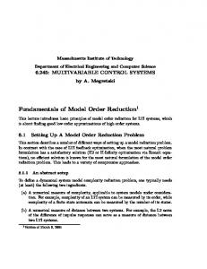
Figure 1: The nonlinear circuit example.

device example, to make clear the nonlinear model reduction problem, and then in Section 3 we describe the existing nonlinear reduction techniques in a more abstract setting. In Section 4, we present the trajectorybased piecewise-linear model order reduction strategy and outline an approach for accelerating the needed simulation. Examples are examined in Section 5, and in Section 6 we present our conclusions.

2. Examples of nonlinear dynamic systems A large class of nonlinear dynamic systems may be described using the following state space approach:  dx  t  dt 

y t



f  x  t  Bu  t  CT x  t 

(1)

where x  t   RN is a vector of states, f : RN RN is a nonlinear vectorvalued function, B is an N  M input matrix, u : R RM is an input signal, C is an N  K output matrix and y : R RK is the output signal. In this paper we will focus on two distinct examples of nonlinear systems which may be described by equations (1) and, due to their highly nonlinear dynamic behavior, illustrate well the challenges associated with nonlinear model order reduction.

In this paper we present an approach to the nonlinear model reduction based on representing the nonlinear system with a piecewise-linear system and then reducing each of the pieces with Krylov subspace projection methods. However, rather than approximating the individual components as piecewise-linear and then composing hundreds of components to make a system with exponentially many different linear regions, we instead generate a small set of linearizations about the state trajectory which is the response to a ”training input”. At first glance, such an approach would seem to work only when all the inputs are very close to the training input, but as examples will show, this is not the case. In fact, the method easily outperforms recently developed techniques based on quadratic reduction.

The first example, considered by Chen et al. [1], is a nonlinear circuit shown in Figure 1. The circuit consists of resistors, capacitors and diodes with a constitutive equation id  v   exp  40v  1.1 For simplicity we assume that all the resistors and capacitors have unit resistance and capacitance, respectively (r  1, C  1). In this case the input is the current source entering node 1: u  t   i  t  and the (single) output is chosen to be the voltage at node 1: y  t   v1  t  .

We start in the next section by describing a circuit and a micromachined

the linear model, considered later on, we assume that id  v  and in the quadratic model – id  v   40v 800v2 .

1 In



40v

by V T yields: 

dz  t  dt  y t  

Figure 2: Micromachined fixed-fixed beam (following Huang et al. [8]). The other example is a micromachined fixed-fixed beam structure shown in Figure 2. Following Huang et al. [8], the dynamic behavior of this coupled electro-mechanical-fluid system can be modeled with 1D Euler’s beam equation and 2D Reynolds’ squeeze film damping equation given below: EI

∂4 u ∂x4 

S

∂2 u ∂x2

w



Felec 

0



∇  1 6K  u3 p∇p  

p  pa  dy  ρ

12µ

∂  pu  ∂t

∂2 u ∂t 2

(2)

(3)

where x, y and z are as shown in Figure 2, E is Young’s modulus, I is the moment of inertia of the beam, S is the stress coefficient, ρ is the density, pa is the ambient pressure, µ is the air viscosity, K is the Knudsen number, w is the width of the beam in y direction, u  u  x  t  is the height of the beam above the substrate, and p  x  y t  is the pressure distribution in the fluid below the beam. The electrostatic force is approximated as2 suming nearly parallel plates and is given by Felec   ε02uwv2 , where v is the applied voltage. Spatial discretization of equations (2) and (3) using a standard finitedifference scheme (cf. [17]) leads to a large nonlinear dynamic system in form (1). In this case the state vector x consists of heights of the beam above the substrate (u) computed at the discrete grid points, their time derivatives, and the values of pressure below the beam. In this case we select our output y  t  as the deflection of the center of the beam from the equilibrium point (y  t  r  t  – cf. Figure 2).

3. Model Order Reduction for nonlinear systems Suppose the initial dynamic system (1) is of order N, i.e. is described by N states. The main goal of model order reduction techniques is to generate a model of this system with q states (where q  N), while preserving accurately the input/output behavior of the original system. Virtually all the numerical model order reduction strategies are based on the concept of projecting the states of the initial system onto a suitably selected reduced order state space. This may also be viewed as performing a change of variables: x  Vz

(4)

where z is a q-th order projection of the state x (of order N) in the reduced order space and V is an N  q orthonormal matrix representing a transformation from the original to the reduced state space. In other words, columns of V define an orthonormal basis which spans the reduced order state space. Substituting (4) in (1) and multiplying the first of the resulting equations

V T f  V z  t  V T Bu  t  CT V z  t 

(5)

There are two key issues concerning representation (5) of the initial dynamic system (1). The first one is selecting a reduced basis V , such that system (5) provides good approximation of the initial system (1). For the linear case (i.e. if f   is a linear transformation), there are a number of methods for determining V . They include: selecting vectors from orthogonalized time-series data [8], computing singular vectors of the underlying differential equation Hankel operator [6] or examining Krylov subspaces [1], [2], [4], [7], [10], [11], [12], [15], [17]. The approach based on using time-series data extends directly to the nonlinear cases, and the Hankel operator and Krylov subspace based strategies can be extended to the nonlinear case using linearization (Taylor’s expansions) of the nonlinear system function f   [1], [2], [11], [17]. The other key issue in applying formulation (5) for reduced order modeling is finding a representation of V T f  V   which allows low-cost storage and fast evaluation. Suppose, N  100  000 and q  10. If no approximations are made to the nonlinear function f   , then computing V T f  V z  requires O  100  000 operations and is too costly. The simplest approximation for f   , which allows O  q  (not O  N  ) storage and evaluation of V T f  V   is based on Taylor’s expansion around the initial state (equilibrium point) x0 : 1 W0  x  x0   x  x0  2 where  is the Kronecker product, and A0 and W0 are, respectively, the Jacobian and the Hessian of f   evaluated at the initial state x0 . This approach leads to the following reduced order models proposed in [1], [2],  the linear case, the reduced order model (5) becomes: [11] and [17]. For f  x 

f  x0  A0  x  x0 

dz  t  dt  y t 

V T f  x0  A0r z V T Bu  t  CT V z  t 

where A0r  V T A0V is a q model is  given by [11]2 : dz  t  dt  y t  



(6)

q matrix. The quadratic reduced order

V T f  x0  A0r z CT V z  t 

1W  2 0r

z  z  V T Bu  t 

(7)

where W0r  V T W0  V  V  is a q  q2 matrix. In the above formulations, due to the fact that the reduced matrices are typically dense and must be represented explicitly, the cost of computing V T f  V z  term and the cost of storing the reduced matrices A0r (A0r and W0r in the quadratic case) are O  q2  (in the linear case) and O  q3  (in the quadratic case). Therefore, although the method based on Taylor’s expansions may be extended to higher orders of nonlinearities [11], this approach is limited in practice to cubic expansions, due to exponentially growing memory and computational costs. For instance, if we consider quartic expansion of order q  10, then the memory storage requirement exceeds q5  100  000 elements, and the computational cost is O  q5  . In most cases it becomes inefficient to use so computationally expensive reduced order models.

4. Piecewise-linear model order reduction As described in the previous section, reduced order models based on Taylor series expansion become prohibitively expensive when the order of included nonlinearity becomes large. On the other hand, a simple linearized reduced order model (6), although computationally inexpensive, 2 An alternative formulation of the quadratic reduced order model is presented in [1]. Both formulations give almost identical results.

may be applied only to weakly nonlinear systems and is usually valid for a very limited range of inputs [17]. This leads us to proposing an approach towards model order reduction based on quasi-piecewise-linear approximations of nonlinear systems. The idea is to represent a system as a combination of linear models, generated at different linearization points in the state space (i.e. different states of the initial nonlinear system). The key issue in this approach is that we will be considering multiple linearizations around suitably selected states of the system, instead on relying on a single expansion around the initial state.

4.1 Piecewise-linear representation Let us assume we have generated s linearized models of the nonlinear system (1), with expansions around states x0   xs ! 1 : dx dt 

f  xi  Ai  x  xi  Bu

where x0 is the initial state of the system and Ai are the Jacobians of f   evaluated at states xi . We now consider a weighted combination of the above models: dx dt

s! 1



∑ w˜ i  x 

i" 0

Figure 3: Generation of the linearized models along a trajectory of a nonlinear system in a 2D state space.

s! 1

∑ w˜ i  x  Ai  x 

f  xi 

i" 0

xi  Bu

(8) (9) as a piecewise-linear reduced order model of nonlinear system (1). Clearly, the procedure presented above provides only an example. Nevertheless, as shown in the following sections, it may be effectively used in practice.

where w˜ i  x  are weights depending on state x. (We assume that, for all x, ∑is" ! 01 w˜ i  x   1.) The choice of weights is discussed later on in this section. Assuming we have already generated a q-th order basis V (cf. (4)) we may consider the following reduced order representation of  system (8): dz dt  y

where Br  V T B, Cr γ &# γ0  γs ! 1 %  '





Ar  w  z  Cr z C T V , Ar

T

z γ  w  z

$# A0r A1r 

V T  f  x0 ( A0 x0 ) V T  f  xs !

T

Br u

(9)

A s!

1 r %

and Air

1 (

As ! 1 xs !



V T AiV ,

1 +*

and # z0  z1 ) zs ! 1 % are representations of linearization points x0   xs ! in the reduced basis: # z0  z1  zs ! 1 % &  #V

T

x0  V T x1   V T xs !

1%

Finally, w  z  ,# w0  z   ws ! 1  z  % is a vector of weights (norm -.- w  z /-0-  1 for all z). At this point we need to find a procedure for computing the weights wi , given current state z and the linearization points zi . We assume that weights wi for the reduced models Ari are computed based on the information about the distances -0- z  zi -.- of the linearization points from the current state z. We require that the ‘dominant’ model A jr is the one corresponding to the linearization point z j which is the closest to the current state of the system. The following procedure of computing wi ensures that the above requirement is satisfied: 1. For i  0 1 s  1  compute: di  -.- z  zi -.- 2 . (Alternatively we may take di  -.- Cr  z  zi 2-.- 2 .) 2. Compute m  min 3 di : i  0 

1

3. For i  0 1 s  1  compute wi

s  1 4 . 



exp  di 5 m 

4.2 Generation of the piecewise-linear model

! 25 

4. Normalize wi . One may note that, in the above procedure, the distribution of weights changes rather ‘sharply’ as the current state z evolves in the state space, i.e. once e.g. z j becomes the point closest to z, then weight w j almost immediately becomes 1. This provides a rationale for referring to model

1

So far it has not been discussed how to generate the weighted model given by (8) or, more specifically, how to select linearization points xi . We may assume that linearization of a nonlinear system, generated at state xi is valid or accurate for a given state x if this state is ‘close enough’ to the linearization point xi , i.e. -0- x  xi -.-6 ε, which means that x lies within a ball (in an N-dimensional space) of radius ε and centered at xi . Suppose we would like to cover an N-dimensional state space with such balls. (Therefore assuring that for any state we will find a valid linearized model.) Then, assuming e.g. that the state space is an Ndimensional hypercube: # 0; 1% 7 # 0; 1%  RN , N  1000 and ε  0  1, the total number of models to be generated would equal roughly 101000 . This is clearly a totally infeasible approach, due to enormous memory and computational costs. Instead of finding linearized models covering the entire N-dimensional state space we propose to generate a collection of models along a single, fixed trajectory of the system.3 This means we generate a trajectory by performing a single simulation of the nonlinear system for a fixed ‘training’ input. (In fact, we may perform a faster approximate simulation, which is discussed later on in this section.) This procedure is depicted in Figure 3. Given a training input signal u  t  and initial state x0 we proceed as follows: 1) We generate a linearized model around state xi (initially i  0); 2) We simulate the behavior of the nonlinear system while -0- x  xi -.-26 δ, i.e. while the current state x is close enough to the last linearization point; 3) We take a new linearization point xi 8 1  x (i :  i 1) and return to step 1). In this procedure we may fix the maximum number of models we want to generate. It should be stressed that this piecewiselinear approach is different from methods presented e.g. in [3] or [9], where piecewise-linear approximations of individual elements of the circuit (e.g. diodes or transistors) are considered and a very large collection of linear models is used. In our algorithm, the piecewise-linear approximation applies to a trajectory of the entire nonlinear system, and therefore the number of linearized models may be kept small. 3 The idea of using a collection of linearized models along e.g. an equilibrium manifold or a given trajectory is also used in design of gain scheduled controllers for nonlinear systems – cf. [14], [16].

System response for step input voltage v(t) = 9H(t) 0

−0.5

−0.5

Center point deflection [microns]

Center point deflection [microns]

System response for step input voltage v(t) = 9H(t) 0

−1

−1.5

−2

0

full nonlinear model, N=880 linear reduced model, q=40 quadratic reduced model, q=40 piecewise−linear reduced model, q=41 0.1

0.2

0.3 Time [ms]

0.4

−1

−1.5

−2

0.5

0.6

0

full nonlinear model, N=880 linear reduced model, q=40 quadratic reduced model, q=40 piecewise−linear reduced model, q=41 0.1

0.2

0.3 Time [ms]

0.4

0.5

0.6

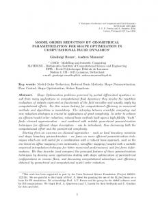
Figure 4: Comparison of system response (micromachined beam example) computed with linear, quadratic and piecewise-linear reduced order models (q  40 and q  41) to the step input voltage u  t 9 9 (t : 0). The piecewise-linear model was generated for the 7-volt step input voltage.

Figure 5: Comparison of system response (micromachined beam example) computed with linear, quadratic and piecewise-linear reduced order models (q  40 and q  41) to the step input voltage u  t ; 9 (t : 0). The piecewise-linear model was generated for the 9-volt step input voltage.

As illustrated in Figure 3, the procedure proposed above allows one to ‘cover with models’ only the part of the state-space located along the ‘training’ trajectory (curve A). Let us assume that the reduced order model (5) is composed of linear models generated along this trajectory. If a certain system’s trajectory, corresponding to a given input signal u, lies within the region of the state space covered by these models, we expect that the constructed piecewise-linear model (5) will suitably approximate the input/output behavior of the initial nonlinear system (cf. curve B).4 It should also be stressed at this point that, although the considered trajectory stays close to the ‘training’ trajectory in the state space, the corresponding input signal can be dynamically very different from the ‘training’ input. In other words, we may apply the piecewise-linear model for inputs which are significantly different from the ‘training’ input, provided the corresponding trajectories stay in the region of the state space covered by the linearized models (cf. results in Section 5).

One may note that the proposed method of generating the piecewiselinear model of a nonlinear dynamic system requires performing simulation of the initial nonlinear system (1) which may be very costly, due to the initial size of the problem. In order to reduce the computational effort we note that it is unnecessary to compute the exact trajectory for the ‘training’ input in order to generate a collection of linearized models. In fact it suffices to compute an approximate trajectory and obtain only approximate linearization points. This leads us to a fast simulation algorithm, which may be summarized in the following points:5 1) Using basis V we construct a reduced order linearized model around state xi (initially i  0); 2) We simulate the reduced order linear system obtained in Step 1 while -.- V z  xi -.- M 4 in the l-th order Krylov subspace: Kl  A0! 1  A0! 1 B  

span 3 A0! 1 B ) A0! l B 4

(11)

5 Details of this fast simulation algorithm, in the context of model order reduction, are to be presented in a forthcoming journal paper. 6 This approach shares features with reduced basis methods for solving parabolic problems [5]

System response for input current i(t) = (cos(2π t/10)+1)/2

using the Arnoldi algorithm [17] (or block Arnoldi algorithm [13] if the number of inputs M : 1). This choice of basis V˜ ensures that l moments of the transfer function of the reduced order linearized model match l moments of the transfer function for the original linearized model (10) [11].

3. We take V as a union of V˜ and vlM 8

1:

V

˜ &# V ; vlM 8 1 %

.

So, the final size of the reduced basis equals q  lM 1. The last two steps ensure that we will be able to represent exactly the initial state x0 in the reduced basis V . (Note that if the initial state of the system is zero, then steps 2 and 3 become unnecessary.) Exact representation of the initial state guarantees that we will correctly start the fast approximate simulation of the nonlinear system in the reduced order space.7

This section presents results of computations using piecewise-linear reduced order models, obtained with the MOR technique proposed in Section 4. Our main goal is to find out whether this technique does really generate a model of our system. Let us recall that, in the proposed MOR algorithm, the model (which basically consists of a collection of reduced order q  q matrices A0r , A1r , ..., A  s ! 1  r ) is obtained by performing a fast simulation for a given training input signal. In order to show that we have indeed generated a model we should verify that it gives correct outputs for not only for the input it was generated with, but also for other inputs. This verification was done experimentally. We considered our nonlinear circuit for N  100 and generated a reduced order piecewise-linear model of order q  10 using a step input i  t   H  t  3  . For this example, the linearization point changed 4 times, therefore our model consisted of 5 reduced order matrices A0r , ..., A4r . The reduced order model was tested for a cosinusoidal input i  t    cos  2πt 5 10 ? 1 5 2. The results are shown in Figure 6. One may note that the output voltage obtained with the piecewise-linear reduced order model accurately approximates the reference voltage (the curves overlap almost perfectly). Figure 7 provides an analogous test for the example of a micromachined fixed-fixed beam described in Section 2. In this case the reduced order model (q  41) was generated for the 8-volt step training input voltage. (The model used 9 linearization points.) Then it was tested for a cosinusoidal input with a 7-volt amplitude. Once again, the transient obtained with the proposed model matches very accurately the reference result obtained with the full nonlinear model of order N  880. Figures 6 and 7 also provide a comparison of the proposed piecewiselinear reduced order model with linear and quadratic reduced models, generated using methods described in [1], [11] and [17]. It is apparent from the graphs that the piecewise-linear reduced order model gives significantly more accurate results than the linear and quadratic reduced order models using Taylor’s expansions around the initial state. It should be stressed at this point that all models (linear, quadratic and piecewiselinear) were of the same order and, moreover, applied the same basis V (obtained with the procedure described in Section 4.3). 7 Above

we presented only the simplest (and the least computationally expensive) algorithm of generating the reduced basis V . One may easily extend this scheme to construct a basis which includes e.g. states used as subsequent linearization points and basis vectors for Krylov subspaces corresponding to these states.

0.015

0.01

0.005

0 0

2

4

6

8

10

Time [s]

Figure 6: Comparison of system response (nonlinear circuit example) computed with linear, quadratic and piecewise-linear reduced order models (of order q  10) for the input current i  t    cos  2πt 5 10  1 5 2. System response for input voltage v(t) = 7cos(4π t) 0 full nonlinear model, N=880 linear reduced model, q=40 quadratic reduced model, q=40 piecewise−linear reduced model, q=41

−0.05 Center point deflection [microns]

5. Computational results

full nonlinear model, N=100 piecewise−linear model (step input), q=10 quadratic reduced model, q=10 linear reduced model, q=10

0.02 Voltage at node 1 [V]

2. We orthonormalize the initial state vector x0 with respect to the columns of V˜ and obtain vector vlM 8 1 . To this end we may use e.g. the SVD algorithm.

0.025

−0.1

−0.15

−0.2

−0.25

−0.3

0

0.1

0.2

0.3 Time [ms]

0.4

0.5

0.6

Figure 7: Comparison of system response (micromachined beam example) computed with linear, quadratic and piecewise-linear reduced order models (of order q  40 and q  41) for the input voltage u  t   7 cos  4πt  . The piecewise-linear model was generated for the 8-volt step input voltage. Table 1 shows a comparison of performance of the discussed MOR techniques and the reduced order solvers. All the algorithms were implemented in Matlab. The tests were performed in a Linux workstation with Pentium III Xeon processor. One may note that performance for linear and piecewise-linear MOR algorithms is comparable. The generation of the quadratic model is significantly more expensive, due to the costly reduction of the Hessian matrix, which requires q2 computations of the matrix-vector product W  x  x  , where W is a full order N  N 2 Hessian matrix (in this case represented implicitly – cf. [1]). The memory complexity of the piecewise-linear reduced order solver is O  sq2  , where s is the number of linearization points. Consequently, the memory cost is roughly s times larger than for the linear reduced order simulator (for which this cost is O  q2  ). The cost of the quadratic reduced order solver is O  q3  (the reduced order Hessian must be stored

MOR method linear MOR quadratic MOR piecewiselinear MOR

Model generation time [s]

Simulation time [s]

44.8

1.18

2756.5

31.5

80.7

8.0

Table 1: Comparison of the times of generation of the reduced model and reduced order simulations for the quadratic and piecewiselinear MOR techniques. The initial problem had size N  1500. The reduced model had size q  30. The tests were run for the nonlinear circuit example.

reduction of nonlinear MEMS devices”, in proceedings of the IEEE International Symposium on Circuits and Systems, pp. 445-8, vol. 2, 2000. [3] C. T. Dikmen, M. M. Alaybeyi, S. Topcu, A. Atalar, E. Sezer, M. A. Tan, R. A. Rohrer, “Piecewise Linear Asymptotic Waveform Evaluation for Transient Simulation of Electronic Circuits”, in proceedings of the International Symposium on Circuits and Systems, pp. 854-857, Singapore, 1991. [4] P. Feldmann, R. W. Freund, “Efficient linear circuit analysis by Pad´e approximation via the Lanczos process”, IEEE Transactions on Computer Aided Design of Integrated Circuits and Systems, vol. 14, pp. 639-649, 1995. [5] E. Gallopoulos, Y. Saad, “Efficient solution of parabolic equations by Krylov approximation methods”, SIAM Journal of Scientific and Statistical Computing, Vol. 13, No. 5, pp. 1236-1264, 1992.

explicitly as a matrix), so if s @ q, then the memory requirements for the piecewise-linear solver are approximately the same as for the quadratic solver. For our examples (cf. Figures 6 and 7), s  5 @ q 5 2 and s  9 @ q 5 4, respectively, so in fact the memory used by the piecewise-linear algorithm equaled roughly only half (and a quarter) of the memory used by the quadratic solver.

[6] K. Glover, “All Optimal Hankel-norm Approximations of Linear Multivariable Systems and Their L∞ error Bounds”, International Journal of Control, Vol. 39, No. 6, pp. 1115-1193, 1984.

6. Conclusions

[8] E. Huang, Y. Yang, S. Senturia, “Low-Order Models For Fast Dynamical Simulation of MEMS Microstructures”, in proceedings of the IEEE International Conference on Solid State Sensors and Actuators (Transducers ’97), Vol. 2, pp. 1101-1104, 1997.

In this paper we have proposed an efficient numerical approach towards automatic model order reduction and simulation of nonlinear systems. The results obtained for the examples of a nonlinear circuit and a micromachined beam indicate that this method provides good accuracy for different applications. The method also proves to be characterized by low computational and memory requirements, therefore providing a cost-efficient alternative for the nonlinear MOR techniques based on linear and quadratic models. Although the algorithm in its current state has proved to be very effective, a number of its aspects require further investigation, including the procedure of merging (weighting) the linearized models or the method of selecting linearization points. There are also many possible extensions of the presented technique, which may include application of multiple reduced bases (instead of a single basis generated at the initial state) in the reduced order piecewise-linear simulators or developing schemes for automatic model generation with multiple ‘training’ inputs, which may allow one to extend the validity of the quasi-piecewise-linear reduced order model to inputs with different scales of amplitudes. It should be stressed that application of the discussed piecewise-linear reduced order approach is not limited to the class of SISO or MIMO dynamic systems found in circuit or MEMS modeling. It may be easily extended for use in macromodeling of second order systems arising in e.g. coupled domain problems involving micromachined electromechanical devices.

[7] E. J. Grimme, D. C. Sorensen, P. Van Dooren, “Model Reduction of State Space Systems via an Implicitly Restarted Lanczos Method”, Numerical Algorithms, vol. 12, no. 1-2, pp. 1-31, 1996.

[9] R. Kao, M. Horowitz, “Timing analysis for Piecewise Linear Rsim”, IEEE Transactions on Computer-Aided Design of Integrated Circuits and Systems, Vol. 13, No. 12, pp. 1498-1512, 1994. [10] A. Odabasioglu, M. Celik, L. Pileggi, “PRIMA: Passive reduced-order interconnect macromodeling algorithm”, in proceedings of the IEEE/ACM International Conference on Computer-Aided Design, pp. 58-65, 1997. [11] J. R. Phillips, “Automated extraction of nonlinear circuit macromodels”, in proceedings of the Custom Integrated Circuit Conference, pp. 451-454, 2000. [12] J. R. Phillips, “Model reduction of time-varying systems using approximate multipoint Krylov-subspace projectors”, in proceedings of the IEEE/ACM International Conference on Computer-Aided Design, pp. 96-102, 1998. [13] D. Ramaswamy, “Automatic Generation of Macromodels for MicroElectroMechanical Systems (MEMS)”, Ph.D. thesis, Massachusetts Institute of Technology, 2001. [14] J. S. Shamma, “Analysis and Design of Gain Scheduled Control Systems”, Ph.D. thesis, Massachusetts Institute of Technology, 1988.

This work was sponsored by the DARPA composite CAD program, the NSF program in computer-aided design, the DARPA muri program, and grants from Synopsys, Compaq and Intel.

[15] L. M. Silveira, M. Kamon, J. White, “Efficient Reduced-Order Modeling of Frequency-Dependent Coupling Inductances associated with 3-D Interconnect Structures”, in proceedings of the European Design and Test Conference, pp. 534-538, 1995.

7. References

[16] D. J. Stilwell, W. J. Rugh, “Interpolation Methods for Gain Scheduling”, in proceedings of the 37th IEEE Conference on Decision and Control, pp. 3003-3008, 1998.

[1] Y. Chen, J. White, “A Quadratic Method for Nonlinear Model Order Reduction”, in proceedings of the International Conference on Modeling and Simulation of Microsystems, pp. 477-480, 2000. [2] J. Chen, S-M. Kang, “An algorithm for automatic model-order

[17] F. Wang, J. White, “Automatic model order reduction of a microdevice using the Arnoldi approach”, in proceedings of the International Mechanical Engineering Congress and Exposition, pp. 527-530, 1998.