Model order reduction for parameter-dependent

THÈSE DE DOCTORAT DE L’ÉCOLE CENTRALE NANTES École doctorale Sciences Pour l’Ingénieur, Géosciences, Architecture

Présentée par

Olivier ZAHM Pour obtenir le grade de DOCTEUR DE L’ÉCOLE CENTRALE NANTES

Sujet de la thèse

Méthodes de réduction de modèle pour les équations paramétrées – Applications à la quantification d’incertitude.

soutenue le 20 novembre 2015, devant le jury composé de : Président: Rapporteurs:

Examinateurs:

Yvon MADAY

Professeur des Universités, Université Paris 6

Fabio NOBILE Christophe PRUD’HOMME

Professeur associé, École Polytechnique Fédérale de Lausanne Professeur des Universités, Université de Strasbourg

Marie BILLAUD-FRIESS Tony LELIÈVRE Anthony NOUY Clémentine PRIEUR

Maître de conférence, École Centrale Nantes (co-encadrant) Professeur à l’École des Ponts ParisTech Professeur des Universités, École Centrale Nantes (directeur) Professeur des Universités, Université Grenoble 1

“Der, welcher wandert diese Straße voll Beschwerden, wird rein durch Feuer, Wasser, Luft und Erden.” — La Flûte enchantée, deuxième acte, vingt-huitième entrée.

À mon épouse Alexandra, pour son amour et son soutien.

Résumé

Les méthodes de réduction de modèle sont incontournables pour la résolution d’équations paramétrées de grande dimension qui apparaissent dans les problèmes de quantification d’incertitude, d’optimisation ou encore les problèmes inverses. Dans cette thèse nous nous intéressons aux méthodes d’approximation de faible rang, notamment aux méthodes de bases réduites et d’approximation de tenseur. L’approximation obtenue par projection de Galerkin peut être de mauvaise qualité lorsque l’opérateur est mal conditionné. Pour les méthodes de projection sur des espaces réduits, nous proposons des préconditionneurs construits par interpolation d’inverse d’opérateur, calculés efficacement par des outils d’algèbre linéaire "randomisée". Des stratégies d’interpolation adaptatives sont proposées pour améliorer soit les estimateurs d’erreur, soit les projections sur les espaces réduits. Pour les méthodes d’approximation de tenseur, nous proposons une formulation en minimum de résidu avec utilisation de norme idéale. L’algorithme de résolution, qui s’interprète comme un algorithme de gradient avec préconditionneur implicite, permet d’obtenir une approximation quasi-optimale de la solution. Enfin nous nous intéressons à l’approximation de quantités d’intérêt à valeur fonctionnelle ou vectorielle. Nous généralisons pour cela les approches de type "primale-duale" au cas non scalaire, et nous proposons de nouvelles méthodes de projection sur espaces réduits. Dans le cadre de l’approximation de tenseur, nous considérons une norme dépendant de l’erreur en quantité d’intérêt afin d’obtenir une approximation de la solution qui tient compte de l’objectif du calcul.

Mots clefs: Réduction de modèle – Quantification d’incertitude – Equations paramétrées – Bases réduites – Approximation de faible rang de tenseur – Préconditionneur – Quantité d’intérêt

Abstract

Model order reduction has become an inescapable tool for the solution of high dimensional parameter-dependent equations arising in uncertainty quantification, optimization or inverse problems. In this thesis we focus on low rank approximation methods, in particular on reduced basis methods and on tensor approximation methods. The approximation obtained by Galerkin projections may be inaccurate when the operator is ill-conditioned. For projection based methods, we propose preconditioners built by interpolation of the operator inverse. We rely on randomized linear algebra for the efficient computation of these preconditioners. Adaptive interpolation strategies are proposed in order to improve either the error estimates or the projection onto reduced spaces. For tensor approximation methods, we propose a minimal residual formulation with ideal residual norms. The proposed algorithm, which can be interpreted as a gradient algorithm with an implicit preconditioner, allows obtaining a quasi-optimal approximation of the solution. Finally, we address the problem of the approximation of vector-valued or functionalvalued quantities of interest. For this purpose we generalize the ’primal-dual’ approaches to the non-scalar case, and we propose new methods for the projection onto reduced spaces. In the context of tensor approximation we consider a norm which depends on the error on the quantity of interest. This allows obtaining approximations of the solution that take into account the objective of the numerical simulation.

Keywords: Model order reduction – Uncertainty quantification – Parameter dependent equations – Reduced Basis – Low rank tensor approximation – Preconditioner – Quantity of interest

Contents Contents 1 Introduction to model order reduction for parameter-dependent equations 1 Context and contributions . . . . . . . . . . . . . . . . . . . . . . . . 1.1 Parameter-dependent equations . . . . . . . . . . . . . . . . . 1.2 Functional approximation of the solution map . . . . . . . . . 1.3 Low-rank approximation of the solution map . . . . . . . . . . 1.4 Contributions and organization of the manuscript . . . . . . . 2 Low-rank methods: a subspace point of view . . . . . . . . . . . . . . 2.1 Projection on a reduced space . . . . . . . . . . . . . . . . . . 2.2 Proper orthogonal decomposition . . . . . . . . . . . . . . . . 2.3 Reduced basis method . . . . . . . . . . . . . . . . . . . . . . 3 Low-rank methods based on tensor approximation . . . . . . . . . . . 3.1 Parameter-dependent equation as a tensor structured equation 3.2 Low-rank tensor formats . . . . . . . . . . . . . . . . . . . . . 3.3 Approximation in low-rank tensor format . . . . . . . . . . . . 2 Interpolation of inverse operators for preconditioning parameterdependent equations 1 Introduction . . . . . . . . . . . . . . . . . . . . . . . . . . . . . . . . 2 Interpolation of the inverse of a parameter-dependent matrix using Frobenius norm projection . . . . . . . . . . . . . . . . . . . . . . . . 2.1 Projection using Frobenius norm . . . . . . . . . . . . . . . . 2.2 Projection using a Frobenius semi-norm . . . . . . . . . . . . 2.3 Ensuring the invertibility of the preconditioner for positive definite matrix . . . . . . . . . . . . . . . . . . . . . . . . . . 2.4 Practical computation of the projection . . . . . . . . . . . . . 3 Preconditioners for projection-based model reduction . . . . . . . . .

i

1 3 3 4 6 7 9 10 11 12 15 16 18 20

29 31 33 33 35 43 45 46

ii

Contents

4

5

6

3.1 Projection of the solution on a given reduced subspace . . . 3.2 Greedy construction of the solution reduced subspace . . . . Selection of the interpolation points . . . . . . . . . . . . . . . . . . 4.1 Greedy approximation of the inverse of a parameter-dependent matrix . . . . . . . . . . . . . . . . . . . . . . . . . . . . . . 4.2 Selection of points for improving the projection on a reduced space . . . . . . . . . . . . . . . . . . . . . . . . . . . . . . . 4.3 Recycling factorizations of operator’s evaluations - Application to reduced basis method . . . . . . . . . . . . . . . . . Numerical results . . . . . . . . . . . . . . . . . . . . . . . . . . . . 5.1 Illustration on a one parameter-dependent model . . . . . . 5.2 Multi-parameter-dependent equation . . . . . . . . . . . . . Conclusion . . . . . . . . . . . . . . . . . . . . . . . . . . . . . . . .

. 47 . 49 . 52 . 52 . 55 . . . . .

55 56 56 61 69

3 Projection-based model order reduction for estimating vector-valued variables of interest 73 1 Introduction . . . . . . . . . . . . . . . . . . . . . . . . . . . . . . . . 75 2 Analysis of different projection methods for the estimation of a variable of interest . . . . . . . . . . . . . . . . . . . . . . . . . . . . . . 76 2.1 Petrov-Galerkin projection . . . . . . . . . . . . . . . . . . . . 76 2.2 Primal-dual approach . . . . . . . . . . . . . . . . . . . . . . . 79 2.3 Saddle point problem . . . . . . . . . . . . . . . . . . . . . . . 82 3 Goal-oriented projections for parameter-dependent equations . . . . . 86 3.1 Error estimates for vector-valued variables of interest . . . . . 87 3.2 Greedy construction of the approximation spaces . . . . . . . 89 4 Numerical results . . . . . . . . . . . . . . . . . . . . . . . . . . . . . 91 4.1 Applications . . . . . . . . . . . . . . . . . . . . . . . . . . . . 91 4.2 Comparison of the projection methods . . . . . . . . . . . . . 94 4.3 Greedy construction of the reduced spaces . . . . . . . . . . . 100 5 Conclusion . . . . . . . . . . . . . . . . . . . . . . . . . . . . . . . . . 104 4 Ideal minimal residual formulation for tensor approximation 1 Introduction . . . . . . . . . . . . . . . . . . . . . . . . . . . . . 2 Functional framework for weakly coercive problems . . . . . . . 2.1 Notations . . . . . . . . . . . . . . . . . . . . . . . . . . 2.2 Weakly coercive problems . . . . . . . . . . . . . . . . . 3 Approximation in low-rank tensor subsets . . . . . . . . . . . . 3.1 Hilbert tensor spaces . . . . . . . . . . . . . . . . . . . .

. . . . . .

. . . . . .

107 . 109 . 112 . 112 . 112 . 113 . 113

Contents

4

5

6

7

8

9

3.2 Classical low-rank tensor subsets . . . . . . . . . . 3.3 Best approximation in tensor subsets . . . . . . . . Minimal residual based approximation . . . . . . . . . . . 4.1 Best approximation with respect to residual norms 4.2 Ideal choice of the residual norm . . . . . . . . . . 4.3 Gradient-type algorithm . . . . . . . . . . . . . . . Perturbation of the ideal approximation . . . . . . . . . . 5.1 Approximation of the ideal approach . . . . . . . . 5.2 Quasi-optimal approximations in Mr (X) . . . . . . 5.3 Perturbed gradient-type algorithm . . . . . . . . . 5.4 Error indicator . . . . . . . . . . . . . . . . . . . . Computational aspects . . . . . . . . . . . . . . . . . . . . 6.1 Best approximation in tensor subsets . . . . . . . . 6.2 Construction of an approximation of Λδ (r) . . . . . 6.3 Summary of the algorithm . . . . . . . . . . . . . . Greedy algorithm . . . . . . . . . . . . . . . . . . . . . . . 7.1 A weak greedy algorithm . . . . . . . . . . . . . . . 7.2 Convergence analysis . . . . . . . . . . . . . . . . . Numerical example . . . . . . . . . . . . . . . . . . . . . . 8.1 Stochastic reaction-advection-diffusion problem . . 8.2 Comparison of minimal residual methods . . . . . . 8.3 Properties of the algorithms . . . . . . . . . . . . . 8.4 Higher dimensional case . . . . . . . . . . . . . . . Conclusion . . . . . . . . . . . . . . . . . . . . . . . . . . .

iii

. . . . . . . . . . . . . . . . . . . . . . . .

. . . . . . . . . . . . . . . . . . . . . . . .

. . . . . . . . . . . . . . . . . . . . . . . .

. . . . . . . . . . . . . . . . . . . . . . . .

. . . . . . . . . . . . . . . . . . . . . . . .

. . . . . . . . . . . . . . . . . . . . . . . .

114 115 116 116 117 118 120 120 121 121 123 124 124 125 129 129 130 131 135 135 136 141 144 148

5 Goal-oriented low-rank approximation for the estimation of vectorvalued quantities of interest 151 1 Introduction . . . . . . . . . . . . . . . . . . . . . . . . . . . . . . . . 153 2 Choice of norms . . . . . . . . . . . . . . . . . . . . . . . . . . . . . . 154 2.1 Natural norms . . . . . . . . . . . . . . . . . . . . . . . . . . . 154 2.2 Goal-oriented norm . . . . . . . . . . . . . . . . . . . . . . . . 156 3 Algorithms for goal-oriented low-rank approximations . . . . . . . . . 157 3.1 Iterative solver with goal-oriented truncations . . . . . . . . . 159 3.2 A method based on an ideal minimal residual formulation . . 160 4 Application to uncertainty quantification . . . . . . . . . . . . . . . . 162 4.1 Linear quantities of interest . . . . . . . . . . . . . . . . . . . 163 4.2 Properties of the norms . . . . . . . . . . . . . . . . . . . . . 164 4.3 Approximation of u(ξ) by interpolation . . . . . . . . . . . . . 166

iv

Contents

5

6 7

Numerical experiments . . . . . . . . . . . . . . . . . . . . . . . . . 5.1 Iterative solver (PCG) with truncations . . . . . . . . . . . . 5.2 Ideal minimal residual formulation . . . . . . . . . . . . . . Conclusion . . . . . . . . . . . . . . . . . . . . . . . . . . . . . . . . Appendix: practical implementation of the approximation operators

Bibliography

. . . . .

168 168 172 177 178 183

Chapter 1 Introduction to model order reduction for parameter-dependent equations

Contents 1

2

3

Context and contributions . . . . . . . . . . . . . . . . . . . .

3

1.1

Parameter-dependent equations . . . . . . . . . . . . . . . . .

3

1.2

Functional approximation of the solution map . . . . . . . . .

4

1.3

Low-rank approximation of the solution map . . . . . . . . .

6

1.4

Contributions and organization of the manuscript . . . . . . .

7

Low-rank methods: a subspace point of view . . . . . . . . .

9

2.1

Projection on a reduced space . . . . . . . . . . . . . . . . . .

10

2.2

Proper orthogonal decomposition . . . . . . . . . . . . . . . .

11

2.3

Reduced basis method . . . . . . . . . . . . . . . . . . . . . .

12

Low-rank methods based on tensor approximation . . . . .

15

3.1

Parameter-dependent equation as a tensor structured equation 16

3.2

Low-rank tensor formats . . . . . . . . . . . . . . . . . . . . .

18

3.3

Approximation in low-rank tensor format . . . . . . . . . . .

20

Context and contributions

1

3


1.1

Parameter-dependent equations

Over the past decades, parameter-dependent equations have received a growing interest in different branches of science and engineering. These equations are typically used for the numerical simulation of physical phenomena governed by partial differential equations (PDEs) with different configurations of the material properties, the shape of the domain, the source terms, the boundary conditions etc. The parameter refers to these data that may vary. Various domains of application involve parameter-dependent equations. For example in optimization or in control, we search the parameter value that minimizes some cost function which is defined as a function of the solution. Real-time simulation requires the solution for different values of the parameter in a limited computational time. In uncertainty quantification, the parameter is considered as a random variable (which reflects uncertainties on the input data), and the goal is either to study the statistical properties of the solution (forward problem), or to identify the distribution law of the parameter from the knowledge of some observations of the solution (inverse problem). Let us consider a generic parameter-dependent equation A(ξ)u(ξ) = b(ξ),

(1.1)

where the parameter ξ = (ξ1 , . . . , ξd ) is assumed to take values in a parameter set Ξ ⊂ Rd which represents the range of variations of ξ. In the present work, we mainly focus on parameter-dependent linear PDEs. The solution u(ξ) belongs to a Hilbert space V (typically a Sobolev space) endowed with a norm k · kV . A(ξ) is a linear operator defined from V to V 0 , the dual space of V 0 , and b(ξ) ∈ V 0 . The function u : ξ 7→ u(ξ) defined from Ξ to V is called the solution map. When considering the numerical solution of a PDE, a discretization scheme (such as the Finite Element Method [52]) yields a finite dimensional problem of size n, which can also be written under the form (1.1) with V either an approximation space V = V h of dimension n, or an algebraic space V = Rn . In the latter case, A(ξ) is a matrix of size n. In the rest of this introductory chapter, we consider for the sake of simplicity that V is a finite dimensional space. When considering complex physical models, solving (1.1) for one value of the parameter requires a call to an expensive numerical solver (e.g. for the numerical solution of a PDE with a finite discretization, we have n 1). This is a limit-

4

Introduction to MOR for parameter-dependent equations

ing factor for the applications that require the solution u(ξ) for many values of the parameter. In this context, different methods have been proposed for the approximation of the solution map. The goal of these methods, often referred as Model Order Reduction (MOR) methods, is to build an approximation of the solution map u that can be rapidly evaluated for any parameter value, and which is sufficiently accurate for the intended applications. This approximation is used as a surrogate for the solution map. In the following sections, we present MOR methods based on functional approximations, and then based on low-rank approximations. Finally, the contributions of the thesis will be outlined.

1.2

Functional approximation of the solution map

Standard approximation methods construct an approximation uN of u on a basis {ψ1 , . . . , ψN } of parameter-dependent functions: uN (ξ) =

N X

vi ψi (ξ).

(1.2)

i=1

When the basis {ψ1 , . . . , ψN } is fixed a priori, the approximation uN linearly depends on the coefficients v1 , . . . , vN : this is a linear approximation method. Different possibilities have been proposed for the computation of uN . For example, one can rely on interpolation (also called stochastic collocation when the parameter is a random variable) [5, 10, 126], on Galerkin projection (also called stochastic Galerkin projection) [62, 97], or on regression [15, 19]. In the seminal work of Ghanem and Spanos [62] polynomial functions were used for the basis {ψ1 , . . . , ψN }. Since then, various types of bases have been considered such as piecewise polynomials [6,46,124], wavelets [93] etc. However, the main difficulty of these approaches is that the number of basis functions N dramatically increases with respect to the dimension d, i.e. the number of parameters. For example, when using polynomial spaces with total degree p, N = (d + p)!/d!p!. As a consequence the complexity of the approximation methods blows up. Since Bellman [12, 13], the expression “curse of dimensionality” refers to such an increase in complexity with respect to the dimension. It is then necessary to exploit particular properties of the solution map for the elaboration of efficient approximation methods. Even if the smoothness of u with respect to ξ is an essential ingredient for its numerical approximation, it is not sufficient to circumvent the curse of dimensionality (see e.g. [104] where it is proven that the approximation of the class of infinitely many times differentiable functions with uniformly bounded


5

derivatives is intractable). In many situations, the parameters ξ1 , . . . , ξd do not have the same importance in the sense that the solution map may present complex variations with respect to some parameters, and simple variations with respect to the others. This anisotropy can be exploited for the construction of a basis that is well adapted to reproduce u, yielding an accurate approximation with a moderate number of basis functions. The idea is for example to put more effort (e.g. higher polynomial degree) for the description of the variations with respect to some parameters. Finding an adapted basis is the principal motivation of the sparse approximation methods, see [61, 99]. Given a dictionary of functions D = {ψα : α ∈ Λ}, where Λ denotes a countable set, sparse approximation of u consists in finding a subset Λr ⊂ Λ of cardinality r such that an element of the form uΛr =

X

vα ψα (ξ)

(1.3)

α∈Λr

approximates well the solution map. The problem of finding the best approximation of the form (1.3) is often referred as the best r-term approximation problem. Since the basis {ψα : α ∈ Λr } is not chosen a priori, this approach is a non linear approximation method, see [48, 50]. For instance, provided u is sufficiently smooth (typically if u admits an analytical extension to a complex domain), Proposition 5.5 in [31] states that there exists an approximation uΛr of the form (1.2) (built by polynomial interpolation) such that sup ku(ξ) − uΛr (ξ)kV ≤ Cr−ρ ,

(1.4)

ξ∈Ξ

where the constants C and ρ depend on the solution map u and on the dimension d. Furthermore, it is shown in [36] that for some particular parameter-dependent equation with infinite dimension d → ∞, exploiting the anisotropy allows to “break” the curse of dimensionality in the sense that the constants C and ρ do not depend on d. However, best r-term approximation problems are known to be combinatorial optimization problems that are NP hard to solve. In practice, the sparse approximation (1.3) can be obtained by using `1 sparsity-inducing penalization techniques [19, 20, 32], or by selecting the basis functions one after the other in a greedy fashion [37, 38, 109]. We refers to [40] for a detailed introduction and analysis of the methods that exploit the anisotropy of u using sparse approximation techniques.

6


1.3

Low-rank approximation of the solution map

In this thesis, we focus on low-rank approximation methods. The principle is to build an approximation of the solution map of the form ur (ξ) =

r X

vi λi (ξ),

(1.5)

i=1

where the coefficients v1 , . . . , vr and the functions λ1 , . . . , λr are not chosen a priori: they are both determined so that ur approximates well the solution map (in a sense that remains to be defined). Note that low-rank approximations (1.5) are very similar to sparse approximations (1.3): the common feature is that the approximation basis ({ψi (ξ)}ri=1 or {λi (ξ)}ri=1 ) is not fixed a priori. However, instead of choosing λ1 , . . . , λr in a dictionary of functions D, they will be selected in a vector space of functions S, typically a Lebesgue space, or an approximation subspace in a Lebesgue space. We detail now some mathematical aspects of low-rank approximations. Let us introduce the Bochner space Lpµ (Ξ; V ) = {v : Ξ 7→ V : kvkp < ∞} where the norm k · kp is defined by 1/p Z p kv(ξ)kV dµ(ξ) if 1 ≤ p < ∞, kvkp = ξ∈Ξ

kvkp = ess sup kv(ξ)kV

if p = ∞.

ξ∈Ξ

Here µ a probability measure (the law of the random variable ξ). The Bochner space Lpµ (Ξ; V ) has a tensor product structure1 Lpµ (Ξ; V ) = V ⊗ S, where S denotes the Lebesgue space Lpµ (Ξ). In the following we adopt the notation: X = V ⊗ S = Lpµ (Ξ; V ).

(1.6)

The elements of X are called tensors. The approximation manifold associated to the elements of the form (1.5) is denoted by ( r ) X Cr (X) = vi ⊗ λi : vi ∈ V, λi ∈ S ⊂ X. i=1

Let us note that any v ∈ X can be interpreted as a linear operator from V 0 to S defined by w 7→ hv, wi, where h·, ·i denotes the duality pair. With this point of view, 1

V ⊗ S = span{v ⊗ λ : v ∈ V, λ ∈ S}, where v ⊗ λ is called an elementary (or a rank-one) tensor, which can be interpreted as the application from Ξ to V defined by ξ 7→ (v ⊗ λ)(ξ) = vλ(ξ).


7

Cr (X) corresponds to the set operators whose rank (i.e. the dimension of the range) (p) is bounded by r. We denote by dr (u) the lowest possible error we can achieve, with respect to the Lpµ (Ξ; V )-norm, by approximating u by an element of Cr (X): d(p) r (u) =

min ku − ur kp .

(1.7)

ur ∈Cr (X)

(∞)

For the applications where the relation (1.4) holds, we deduce2 that dr (u) ≤ Cr−ρ . p Since the L∞ µ (Ξ; V )-norm is stronger that the Lµ (Ξ; V )-norm, we have (∞) d(p) r (u) ≤ dr (u)

for any 1 ≤ p ≤ ∞. The value of p determines in which sense we want to approximate u. In practice, low-rank approximation methods are either based on p = ∞ or on p = 2. The choice p = ∞ yields an approximation ur of u which is uniformly accurate over Ξ, meaning ku(ξ) − ur (ξ)kV ≤ ε for any ξ ∈ Ξ. This is the natural framework for applications such as rare event estimation or optimization. The choice p = 2 is natural in the stochastic context when the first moments of the solution (e.g. the mean, the variance etc) have to be computed. But in the literature, we observe that the choice of p is generally not driven by the application. For example, approximations built by a method based on p = 2 can be used to provide “numerical charts” [34], while approximations built by a method based on p = ∞ are used in [23] for computing moments of u. In fact, under some assumptions on the smoothness of the solution map, the approximation error measured with the L∞ µ (Ξ; V )-norm can be controlled 2 by the one measured with the Lµ (Ξ; V )-norm (see [77]).

1.4

Contributions and organization of the manuscript

This thesis contains different contributions for the two main low-rank approximation methods, namely the Reduced Basis method (which is here presented as a lowrank method with a subspace point of view) and the methods based on tensor approximation techniques. These contributions address the following issues. • The fact is that the solution map is not known a priori, but implicitly defined as the solution of (1.1). As a consequence, low-rank approximation methods are not able to provide optimal approximations, but only quasi-optimal 2

(∞)

In some applications we rather observe an exponential rate of convergence dr C exp(−crρ ).

(u) ≤

8


approximations in the best case scenario. This loss of accuracy can be problematic for the efficiency of the methods. • In many applications, we only need a partial information (called a quantity of interest) which is a function of the solution map. The challenge is to develop goal-oriented approximation methods which take advantage of such situation in order to reduce the complexity. The organization of the present manuscript is as follow. Chapter 2. We observe in practice that a bad condition number of the operator A(ξ) may yield inefficient model order reduction: the use of a preconditioner P (ξ) ≈ A(ξ)−1 is necessary to obtain accurate approximations. In Chapter 2, we propose a parameter-dependent preconditioner defined as an interpolation of A(ξ)−1 (here we consider that equation (1.1) is an algebraic equation, i.e. A(ξ) is a matrix). This interpolation is defined by a projection method based on the Frobenius norm. Here we use tools of the randomized numerical linear algebra (see [79] for an introduction) for handling large matrices. We propose strategies for the selection of the interpolation points which are dedicated either to the improvement of Galerkin projections or to the estimation of projection errors. Then we show how such preconditioner can be used for projection-based MOR, such as the reduced basis method or the proper orthogonal decomposition method. Chapter 3. In many situations, one is not interested in the solution u(ξ) itself but rather in some variable of interest defined as a function ξ 7→ l(u(ξ)). In the case where l ∈ L(V, R) is a linear function taking scalar values, approximations of the variable of interest can be obtained using a primal-dual approach which consists in computing an approximation of the so-called dual variable. In chapter 3, we extend this approach to functional-valued or vector-valued variables of interest, i.e. l ∈ L(V, Z) where Z is a vector space. In particular we develop a new projection method based on a saddle point formulation for the approximation of the primal and dual variables in reduced spaces. Chapter 4. Low-rank approximations can be obtained through the direct minimization of the residual norm associated to an equation formulated in a tensor product space. In practice, the resulting approximation can be far from being optimal with respect to the norm of interest. In Chapter 4, we introduce an ideal minimal residual formulation such that the optimality of the approximation is achieved with

Low-rank methods: a subspace point of view

9

respect to a desired norm, and in particular the natural norm of L2µ (Ξ; V ) for applications to parameter-dependent equations. We propose and analyze an algorithm which provides a quasi-optimal low-rank approximation of the solution map. Chapter 5. As in Chapter 3, we address the problem of the estimation of a functional-valued (or vector-valued) quantity of interest, which is here defined as L(u) where L ∈ L(X, Z). For example when ξ is a random variable, L(u) can be the conditional expectation E(u(ξ)|ξτ ) with respect to a subset of random variables ξτ . For this purpose, we propose an original strategy which relies on a goal-oriented norm, meaning a norm on X that takes into account the quantity of interest we want to compute. However, the best approximation problem with respect to this norm can not be solved directly. We propose an algorithm that relies on the ideal minimal residual formulation introduced in Chapter 4. The rest of this chapter gives the basic notions of low-rank approximation methods which will be useful for the rest of the manuscript. We distinguish here the low-rank methods with a subspace point of view, such as the Reduced Basis method or the Proper Orthogonal Decomposition method, and the methods based on tensor approximation techniques.

2


Let us note that the subset of tensors with rank bounded by r can be equivalently defined by Cr (X) = {Vr ⊗ S : Vr ⊂ V, dim(Vr ) = r} , so that we have min ku − ur kp =

ur ∈Cr (X)

min

min ku − ur kp .

Vr ⊂V ur ∈Vr ⊗S dim(Vr )=r

This alternative formulation of the low-rank approximation problem suggests to find a subspace Vr ⊂ V of dimension r, often called the reduced space, that minimizes minur ∈Vr ⊗S ku−ur kp . In practice a subspace can be constructed based on the knowledge of snapshots of the solution {u(ξ 1 ), u(ξ 2 ), . . .}. This is the basic idea of the Proper Orthogonal Decomposition (POD) and of the Reduced Basis (RB) methods. The main difference is that the POD method aims at constructing a subspace Vr that is optimal with respect to the L2µ (Ξ; V )-norm (p = 2), whereas the RB method

10


tries to achieve the optimality with respect to the L∞ µ (Ξ; V )-norm (p = ∞). For a given reduced space Vr and for any parameter value ξ ∈ Ξ, the approximation ur (ξ) can be computed by a Galerkin-type projection (i.e. using equation (1.1)) of the solution u(ξ) onto Vr . The term projection-based model order reduction is used for such strategies relying on a projection of the solution onto a reduced space. Note that we do not introduce any approximation space for S.

2.1

Projection on a reduced space

In this sub-section, we assume that we are given a reduced space Vr ⊂ V . The best approximation problem in Vr ⊗ S is: min ku − vr kp = ku − ΠVr ukp ,

vr ∈Vr ⊗S

where ΠVr denotes the V -orthogonal projector onto Vr . For the computation of (ΠVr u)(ξ) = ΠVr u(ξ), we need to know the solution u(ξ). To avoid this, we define ur (ξ) as the Galerkin projection of u(ξ) onto the reduced space Vr . Here we assume that the operator A(ξ) satisfies α(ξ) = inf

v∈V

hA(ξ)v, wi hA(ξ)v, vi > 0 and β(ξ) = sup sup < ∞. 2 kvkV v∈V w∈V kvkV kwkV

(1.8)

The Galerkin projection ur (ξ) ∈ Vr is characterized by hA(ξ)ur (ξ), vi = hb(ξ), vi

(1.9)

for all v ∈ Vr . Computing ur (ξ) requires the solution of a small3 linear system of size r called the reduced system. Céa’s lemma provides the following quasi-optimality result: ku(ξ) − ur (ξ)kX ≤ κ(ξ)ku(ξ) − ΠVr u(ξ)kV , (1.10) where κ(ξ) = β(ξ)/α(ξ) ≥ 1 is the condition number of A(ξ). Then we have ku − ur kp ≤ κ min ku − vr kp vr ∈Vr ⊗S

with κ = supξ∈Ξ κ(ξ). We note that a bad condition number for A(ξ) can lead to an inaccurate Galerkin projection. One can find in [42] a Petrov-Galerkin projection method that aims at defining a better projection onto the reduced space by constructing a suitable test space. 3

By small, we mean that r n, where we recall that n denotes the dimension of the “full” problem (1.1).


11

In order to have a rapid evaluation of ur (ξ) for any parameter value ξ ∈ Ξ, the complexity for solving (1.9) should be independent of n (i.e. the complexity of the original problem). To obtain this property, a key ingredient is that both the operator A(ξ) and the right hand side b(ξ) admit an affine decomposition with respect to the parameter ξ, meaning that A(ξ) =

mA X

Ak ΦA k (ξ)

,

b(ξ) =

k=1

mb X

bk Φbk (ξ),

(1.11)

k=1

b where ΦA k and Φk are scalar valued functions. Such decomposition allows to precompute the reduced operators (resp. right hand sides) associated to Ak (resp. to bk ) during the so called Offline phase. Then for any ξ ∈ Ξ the reduced system can be rapidly reassembled (using (1.11)) and solved during the Online phase, with a complexity that is independent of n. If A(ξ) and b(ξ) do not have an affine decomposition, one can use techniques such as the Empirical Interpolation Method [9] to build approximations of A(ξ) and b(ξ) of the form (1.11). Moreover, if such decompositions exist but the operators Ak or the vectors bk are not available (for example in a non-intrusive setting), one can use the technique proposed in [29] for the computation of affine decompositions from evaluations of A(ξ) and b(ξ).

2.2

Proper orthogonal decomposition

We present now the principle of the POD. This method was first introduced for the analysis of turbulent flows in fluid mechanics [14]. We refer to [84] for an introduction in the context of parameter-dependent equations. We assume that the solution map u belongs to L2µ (Ξ; V ) (p = 2), and we consider P its singular value decomposition4 u = ∞ i=1 σi vi ⊗ λi , where σi ∈ R are the singular values (sorted in decreasing order) and vi ∈ V , λi ∈ S are the corresponding left and right singular vectors. This decomposition is also called the Karhunen-Loève expansion when ξ is a random variable. An important feature of this decomposition is that the truncation to its first r terms gives an optimal rank-r approximation of u with respect to the L2µ (Ξ; V )-norm: ku −

r X

σi vi ⊗ λi k2 = min ku − vr k2 .

i=1

vr ∈Cr (X)

(1.12)

As a consequence, the optimal reduced space Vr is given by the span of the dominant left singular vectors {v1 , . . . , vr }. The idea of the POD is to approach the k · k2 -norm 4

Note that since dim(V ) < ∞, the sum is finite.

12


of equation (1.12) using the Monte Carlo method for the estimation of the integral over Ξ:

ku −

vr k22

Z ku(ξ) −

=

vr (ξ)k2V dµ(ξ)

Ξ

K 1 X ≈ ku(ξ k ) − vr (ξ k )k2V K k=1

(1.13)

where ξ 1 , . . . , ξ K are K independent realizations of a random variable whose probability law is µ. A reduced space Vr is then defined as the span of the first r left singular vectors of the operator K 1 X λ ∈ R 7→ u(ξ k )λk ∈ V. K k=1 K

When V = Rn , this operator corresponds to a matrix whose columns are the snapshots u(ξ 1 ), . . . , u(ξ K ). Then, efficient algorithms are available for the computation of the complete SVD [69], or for the computation of the truncated SVD [68]. Remark 2.1 (Goal-oriented POD). Alternative constructions of the reduced space have been proposed in order to obtain accurate approximations of some variable of interest defined by l(u(ξ)), where l ∈ L(V, Z) is a linear function taking values in a vector space Z = Rm . The idea proposed in [28] is to replace the norm k · kV by a semi-norm kl(·)kZ in the expression (1.13), so that the optimality of the reduced space is achieved with respect to the quantity of interest we want to compute. However such strategy does not take into account the projection problem on the resulting reduced space, and there is no guaranty that such a strategy improves the approximation of the quantity of interest. We believe that the computation of a goal-oriented projection of u(ξ) is as important as the computation of a goal-oriented reduced space (see Chapter 3).

2.3

Reduced basis method

The motivation of the RB method is to build a reduced space which provides a controlled approximation of the solution map with respect to the L∞ µ (Ξ; V )-norm (∞) (p = ∞). The lowest error dr (u) for the approximation of u by a rank r element


13

satisfies d(∞) r (u) = = =

min

min sup ku(ξ) − vr (ξ)kV ,

vr ∈Vr ⊗S ξ∈Ξ Vr ⊂V dim(Vr )=r

min

sup min ku(ξ) − vr kV ,

min

sup min kw − vr kV ,

Vr ⊂V ξ∈Ξ vr ∈Vr dim(Vr )=r

Vr ⊂V w∈M vr ∈Vr dim(Vr )=r

(∞)

where M = {u(ξ) : ξ ∈ Ξ} ⊂ V denotes the solution manifold. Then dr (u) is the Kolmogorov r-width of M, see [88]. There is no practical algorithm to compute the corresponding optimal subspace, even if we had access to the solution u(ξ) for any ξ ∈ Ξ. The idea of the RB method is to construct Vr as the span of snapshots of the solution. Contrarily to the POD method which relies on a crude Monte Carlo sampling of the solution manifold, the RB method selects the evaluation points adaptively. In the seminal work [123], a Greedy algorithm has been proposed for the construction of the approximation space Vr+1 = Vr + span{u(ξ r+1 )}. Ideally, ξ r+1 should be chosen where the error of the current approximation ur (ξ) is maximal, that means ξ r+1 ∈ arg max ku(ξ) − ur (ξ)kV . ξ∈Ξ

(1.14)

Since ur+1 (ξ) is defined as the Galerkin projection of u(ξ) onto a subspace Vr+1 which contains u(ξ r+1 ), and thanks to relation (1.10), we have ku(ξ r+1 ) − ur+1 (ξ r+1 )kV = 0 (in fact, we also have ku(ξ)−ur+1 (ξ)kV = 0 for any ξ ∈ {ξ 1 , . . . , ξ r+1 }, so that ur+1 (ξ) is an interpolation of u(ξ) on the set of points {ξ 1 , . . . , ξ r+1 }). We understand that this approach aims at decreasing the L∞ µ (Ξ; V ) error. But in practice, the selection strategy (1.14) is unfeasible since it requires the solution u(ξ) for all ξ ∈ Ξ. To overcome such an issue, the exact error ku(ξ) − ur (ξ)kV is replaced by an estimator ∆r (ξ) that can be computed for any ξ ∈ Ξ with low computational costs. This estimator is said to be tight if there exist two constants c > 0 and C < ∞ such that c∆r (ξ) ≤ ku(ξ) − ur (ξ)kV ≤ C∆r (ξ) holds for any ξ ∈ Ξ. A popular error estimator is the dual norm of the residual ∆r (ξ) = kA(ξ)ur (ξ) − b(ξ)kV 0 . In that case, we have c = inf ξ β(ξ)−1 and C = supξ α(ξ)−1 where α(ξ) and β(ξ) the constants defined in (1.8).

14


Remark 2.2 (Training set). In practice, Ξ is replaced by a training set Ξtrain with finite cardinality, but large enough to represent well Ξ in order not to miss relevant parts of the parameter domain. This Greedy algorithm has been analyzed in several papers [18, 25, 49, 95]. In particular, Corollary 3.3 in [49] states that if the Kolmogorov r-width satisfies (∞) dr (u) ≤ C0 r−ρ for some C0 > 0 and ρ > 0, then the resulting approximation space Vr satisfies min ku − vr k∞ ≤ γ −2 C1 r−ρ (1.15) vr ∈Vr ⊗S

(∞)

with C1 = 25ρ+1 C0 and γ = c/C ≤ 1. Moreover, if dr (u) = C0 exp(−c0 rρ ) for some positive constants C0 , c0 and ρ, then min ku − vr k∞ ≤ γ −1 C1 exp(−c1 rρ )

vr ∈Vr ⊗S

(1.16)

√ with C1 = 2C0 and c1 = 2−1−2ρ c0 . Qualitatively, these results tell us that the RB method is particularly interesting in the sense that it preserves (in some situations) the convergence rate of the Kolmogorov r-width. But from a quantitative point of view, a constant γ close to zero may deteriorate the quality of Vr for small r. Let us note that when the error estimator is the dual norm of the residual (i.e. ∆r (ξ) = kA(ξ)ur (ξ) − b(ξ)kV 0 ), we have γ −1 =

supξ β(ξ) β(ξ) C = ≥ sup =: κ. c inf ξ α(ξ) ξ α(ξ)

Here again, the condition number of A(ξ) plays an important role on the quality of the approximation space Vr . If it is large, then γ −1 will be also large. Furthermore, note that we have supξ (β(ξ)α(ξ)/α(ξ)) supξ α(ξ) γ −1 = ≤ κ. inf ξ α(ξ) inf ξ α(ξ) Even with an ideal condition number κ = 1, we have no guaranty that the constant γ −1 will be close to one (take for example A(ξ) = ξI, where I is the identity operator and 0 < ε ≤ ξ ≤ 1. Then κ(ξ) = 1 and γ −1 = ε−1 ). Remark 2.3 (Certified RB). In order to have a certified error bound, one can use the error estimator ∆r (ξ) = α(ξ)−1 kA(ξ)ur (ξ) − b(ξ)kV 0 which provides an upper bound of the error: ku(ξ) − ur (ξ)kV ≤ ∆r (ξ). This corresponds to the Certified Reduced Basis method [114, 123]. Then we have C = 1, c = inf ξ α(ξ)/β(ξ) and finally γ −1 = κ. Except for the particular case where α(ξ) is given for free, one can build a lower bound αLB (ξ) ≤ α(ξ) using for example the Suc-

Low-rank methods based on tensor approximation

15

cessive Constraint linear optimization Method (SCM), see [83]. Then for ∆r (ξ) = αLB (ξ)−1 kA(ξ)ur (ξ) − b(ξ)kV 0 , the relation ku(ξ) − ur (ξ)kV ≤ ∆r (ξ) still holds and we obtain supξ α(ξ)/αLB (ξ) κ ≤ γ −1 ≤ κ. inf ξ α(ξ)/αLB (ξ)

Remark 2.4 (Goal-oriented RB). For some applications, one is interested in some “region of interest” in the parameter domain Ξ. For example in optimization, we need an accurate approximation of u(ξ) around the minimizer of some cost function ξ 7→ J(u(ξ)). Another example can be found in rare events estimation, where an accurate approximation is needed only in the border of some failure domain defined by {ξ ∈ Ξ : l(u(ξ)) > 0}. The idea proposed in [30] consists in using a weighted error estimate wr (ξ)∆r (ξ), where wr is a positive function that assigns more importance of the error associated to some region of the parameter domain. For rare event estimation, this function can be defined as wr (ξ) = 1/|l(ur (ξ))|.

3


In this section we show how a low-rank approximation of the solution map can be obtained using tensor approximation methods. Here, the principle is to interpret u as the solution of a linear equation Au = B,

(1.17)

which is formulated on the tensor product space X = V ⊗ S endowed with the L2µ (Ξ; V )-norm (p = 2). Contrarily to the subspace point of view presented in Section 2, we build here an explicit representation of ur , meaning that the functions λ1 , . . . , λr will be explicitly computed. In practice this requires to introduce an approximation space for S, such as a polynomial space, a piecewise polynomial space etc, or to work on a sample set (meaning a set Ξtrain ⊂ Ξ of finite cardinality). But, as mentioned in section 1.2, the dimension of such spaces blows up with the number d of parameter. In order to avoid the construction of an approximation space for multivariate functions, we can rather consider ur of the form ur (ξ) =

r X i=1

(1)

(d)

vi λi (ξ1 ) . . . λi (ξd ),

(1.18)

16


which is a so-called separated representation. This requires to introduce approximation spaces only for univariate functions. Here, (1.18) is an approximation in the canonical tensor format with a canonical rank bounded by r, which is known to have bad topological properties. Alternative low-rank formats have been proposed, such as the Tucker format, the Hierarchical Tucker format or the Tensor Train format. In the rest of this section, we first show how the parameter-dependent equation (1.1) can be written as a tensor structured equation (1.17). Then we introduce standard low-rank formats, and we present different methods for the solution of (1.17) using low-rank tensor techniques.

3.1

Parameter-dependent equation as a tensor structured equation

The weak formulation of the parameter-dependent equation (1.1) consists in finding u ∈ X such that Z Z (1.19) hA(ξ)u(ξ), w(ξ)i dµ(ξ) = hb(ξ), w(ξ)i dµ(ξ) Ξ

Ξ

for any w ∈ X. We introduce the operator A : X → X 0 and B ∈ X 0 defined by: Z Z hAv, wi = hA(ξ)v(ξ), w(ξ)i dµ(ξ) and hB, wi = hb(ξ), w(ξ)i dµ(ξ), Ξ

Ξ

for any v, w ∈ X, so that (1.19) can be equivalently written as in equation (1.17). Here, we endow X with the norm k · kX = k · k2 . Then X is a Hilbert space, which is convenient in the present context. A sufficient condition for problem (1.17) to be well-posed is α = inf α(ξ) > 0 and β = sup β(ξ) < ∞, ξ∈Ξ

ξ∈Ξ

where α(ξ) and β(ξ) are defined by (1.8). Indeed, this implies Z Z 2 hAv, vi ≥ α(ξ)kv(ξ)kV dµ(ξ) ≥ α kv(ξ)k2V dµ(ξ) = αkvk2X

(1.20)

Ξ

Ξ

for any v ∈ X, and Z hAv, wi ≤

β(ξ)kv(ξ)kV kw(ξ)kV dµ(ξ) ≤ βkvkX kwkX

(1.21)

Ξ

for any v, w ∈ X. Equations (1.20) and (1.21) ensure respectively the coercivity and the continuity of A on X. Thanks to Lax-Milgram theorem, (1.17) is then well


17

posed. Furthermore, the weak formulation (1.19) (or equivalently (1.17)) is convee in X (for example X e = V ⊗ Se ⊂ X, nient to introduce an approximation space X e in (1.19), the resulting sowith Se ⊂ S a polynomial space). Replacing X by X e (sometimes called the Spectral lution u e is the Galerkin approximation of u onto X Stochastic Galerkin approximation). In the following, we continue working in the e at any time. space X = V ⊗ S, although it can be replaced by X As mentioned earlier, we also want to introduce low-rank approximations of the form (1.18). This is made possible by the fact that, under some assumptions, the space S also admits a tensor product structure. Let us assume that Ξ admits a product structure Ξ = Ξ1 × . . . × Ξd , where Ξν ⊂ R for all ν ∈ {1, . . . , d}, and that Q the measure µ satisfies µ(ξ) = dν=1 µ(ν) (ξν ) for any ξ ∈ Ξ (if µ is the probability law of ξ = (ξ1 , . . . , ξd ), that means that the random variables ξ1 , . . . , ξd are mutually independent). Then the space S has the following tensor product structure5 S = S1 ⊗ . . . ⊗ Sd , where Sν = L2µ(ν) (Ξν ). We discuss now the tensor structure of the operator A and the right-hand side B. We assume here that A(ξ) and b(ξ) admit the following affine decompositions: A(ξ) =

mA X

Ak

k=1

d Y

ΦA k,ν (ξν )

and b(ξ) =

ν=1

mb X k=1

bk

d Y

Φbk,ν (ξν ),

ν=1

b where ΦA k,ν and Φk,ν are scalar valued functions defined over Ξν . This decomposition is similar to the previous one (1.11), but with an additional assumption for the b functions ΦA k and Φk . Then A and B admit the following decompositions

A=

mA X

Ak ⊗

(1) Ak

⊗ ... ⊗

(d) Ak

k=1 (ν)

and B =

mb X

(1)

(d)

b k ⊗ bk ⊗ . . . ⊗ bk ,

k=1 (ν)

where Ak : Sν → Sν0 and bk ∈ Sν0 are defined by Z (ν) (ν) hAk λ, γi = ΦA k,ν (ξν )λ(ξν )γ(ξν ) dµ (ξν ), ZΞν (ν) hbk , γi = Φbk,ν (ξν )γ(ξν ) dµ(ν) (ξν ), Ξν

for all λ, γ ∈ Sν . 5

Here again, Sν can be replaced by an approximation space Seν ⊂ Sν . In that case, the approximation space Se = Se1 ⊗ . . . ⊗ Sed preserves the tensor product structure of S.

18


Thereafter, and for the sake of simplicity, we adopt the notation X = X1 ⊗ . . . ⊗ Xd , where X1 = V , X2 = L2µ(1) (Ξ1 ), X3 = L2µ(2) (Ξ2 ) and so on. Let us note that with this new notation, we have replaced d + 1 by d. Then, A and B are interpreted as tensors: mA O mB O d d X X (ν) (ν) A= Ak and B = Bk . (1.22) k=1 ν=1

3.2

k=1 ν=1

Low-rank tensor formats

We present here different low-rank tensor formats. We refer to the monograph [76] for a detailed presentation. The most simple low-rank tensor format is the canonical rank-r tensor format that is defined by ( r ) X (1) (d) (ν) Cr (X) = xi ⊗ . . . ⊗ xi : xi ∈ X ν . (1.23) i=1

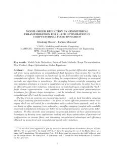
This allows us to define the canonical rank of a tensor x ∈ X as the minimal integer r ∈ N such that x ∈ Cr (X). We use the notation r = rank(x). However, Cr (X) is not a closed subset for d > 2 and r > 1. As shown in [45, proposition 4.6], for some tensor x ∈ C3 (X) such that x ∈ / C2 (X), there exists a tensor y ∈ C2 (X) that can be arbitrarily closed to x. This is an issue for the elaboration of a robust approximation method in this subset. Now we introduce other low-rank tensor formats that have better properties. A key ingredient is the notion of t-rank of a tensor x ∈ X, see [71, 78]. Here, t ⊂ D = {1, . . . , d} denotes a subset of indices, and tc = D\t is the complementary of t in N N D. We consider Xt = ν∈t Xν and Xtc = ν∈tc Xν , so that any x ∈ X ≡ Xt ⊗ Xtc can be interpreted as a tensor of order 2. This process is called the matricization of the tensor with respect to t. Then, we can define the t-rank of a tensor x as the minimal integer r ∈ N such that x ∈ Cr (Xt ⊗ Xtc ) (which is the unique notion of the rank for a tensor of order 2). We then use the notation r = rankt (x) (note that rankt (x) = ranktc (x)). This allows us to introduce the subset of tensors with a Tucker rank bounded by r n o Tr (X) = x ∈ X : rankt (x) ≤ rt , t ∈ D , where r = (r1 , . . . , rd ) ∈ Nd . As a matter of fact, this subset is closed since it T is a finite intersection of closed subsets: Tr (X) = t∈D {x ∈ X : rankt (x) ≤ rt }.


19

Furthermore, any element of xr ∈ Tr (X) can be written xr =

r1 X

...

i1 =1

rd X

(d)

(1)

ai1 ,...,id xi1 ⊗ . . . ⊗ xid ,

(1.24)

id =1 (ν)

where a ∈ Rr1 ×...×rd is called the core tensor, and xiν ∈ Xν for all iν ∈ {1, . . . , rν } and ν ∈ {1, . . . , d}. The format (1.24) is called the Tucker format. However this tensor format suffers from the curse of dimensionality, since the tensor core belongs to a space whose dimension increases exponentially with respect to d: Q dim(Rr1 ×...×rd ) = dν=1 rν . To avoid this, low-rank structure also have to be imposed on the core tensor a. This can be done by considering a dimension tree T ⊂ 2D that is a hierarchical partition of set of dimension D. Examples of such trees are given on Figure 1.1 (we refer to Definition 3.1 in [71] for the definition of such dimension trees). The subset of tensors with Hierarchical Tucker rank bounded by r ∈ N#(T )−1 , first introduced in [78], is defined by n o HrT (X) = x ∈ X : rankt (x) ≤ rt , t ∈ T \D . (1.25) If T is the one-level tree of Figure 1.1(a), then HrT (X) is nothing but Tr (X). When T is the unbalanced tree of Figure 1.1(c), any tensor xr ∈ HrT (X) can be written as in (1.24) with a core a having the following structure: a rd−1

a

ai1 ,...,id =

r1 X k1 =1

...

X

(1)

(2)

(d−1)

(d)

ai1 ,k1 ak1 ,i2 ,k2 . . . akd−2 ,id−1 ,kd−1 akd−1 ,id ,

(1.26)

kd−1 =1

where we used the notations r1a = rank{1} (x), r2a = rank{1,2} (x), and so on6 . Here a a the tensor core a is a chained product of the tensors a(ν) ∈ Sν = Rrν−1 ×rν ×rν (with the convention r0a = rda = 1). The amount of memory for the storage of the core a is P a dim(×dν=1 Sν ) = dν=1 rν−1 rν rνa , which linearly depends on d. Let us mention that for general trees like the balanced tree of Figure 1.1(b), the tensor core possesses also a simple parametrization, see [71, 78] for more information. When considering binary trees (each node has 2 sons), the storage requirement for a also linearly depends on d. Remark 3.1. In fact, the trees presented on Figures 1.1(b) and 1.1(c) yield the same low-rank tensor subset HrT (X): they are both associated to subsets of tensors with bounded t-ranks for t ∈ {{1}, {2}, {3}, {4}, {1, 2}}. Indeed, for the balanced tree 1.1(b) we have rank{1,2} (x) = rank{3,4} (x) to that we can remove the condi6

here, we changed the notations by taking the complementary of the interior nodes of the tree 1.1(c): for example r2a = rank{1,2} (x) = rank{3,...,d} (x).

20


{1, 2, 3, 4}

{1, 2, 3, 4}

{1, 2, 3, 4} {1}

{1, 2}

{2, 3, 4}

{3, 4} {2}

{1} {2} {3} {4} (a) One-level tree (Tucker format).

{3, 4}

{1} {2} {3} {4}

{3}

{4}

(b) Balanced tree (Hierarchical format).

(c) Unbalanced tree (Tensor Train format).

Figure 1.1: Different dimension trees for d = 4. tion on the t-rank for t = {3, 4}, the same for the unbalanced tree 1.1(c) with rank{2,3,4} (x) = rank{1} (x). This is a particular case that can obviously not be generalized to higher dimensions d > 4. We conclude this section by introducing the Tensor Train format (see [105,106]). The subset of tensors with TT-rank bounded by r ∈ Nd−1 is defined by n o T T r (X) = x ∈ X : rankt ≤ rt , t ∈ {1}, {1, 2}, . . . , {1, . . . , d − 1} . This format is a Hierarchical Tucker format associated to a dimension tree of the form given in Figure 1.1(c) with inactive constraints on the t-rank for t ∈ {{2}, . . . , {d− 1}}. Any xr ∈ T T r (X) can be written under the form xr =

r1 X k1 =1

3.3

rd−1

...

X kd−1

(1)

(2)

(d−1)

(d)

xk1 ⊗ xk1 ,k2 ⊗ . . . ⊗ xkd−2 ,kd−1 ⊗ xkd−1 . |{z} | {z } | {z } | {z } =1 ∈X1

∈X2

∈Xd−1

(1.27)

∈Xd

Approximation in low-rank tensor format

We discuss now the problem of approximating a tensor x ∈ X in a low-rank tensor subset Mr (X) ∈ {Cr (X), Tr (X), HrT (X), T T r (X)}. In this section, we emphases on two situations: (a) for a given rank r, we want to find the best approximation of x in the set Mr (X), and (b) for a given ε > 0, we want to perform an approximation xr ∈ Mr (X) such that kx − xr kX ≤ ε with an adapted rank r. Moreover, two cases have to be considered: either the tensor x is known explicitly, or the tensor x is a priori unknown but is the solution of the equation (1.17). In this latter case, we use the notation x = u and xr = ur .


3.3.1

21

Methods based on singular value decomposition

We show how to address both points (a) and (b) for the approximation of a given tensor x using the Singular Value Decomposition (SVD). A key assumption is that the norm k · kX satisfies the relation kx(1) ⊗ . . . ⊗ x(d) kX = kx(1) kX1 . . . kx(d) kXd

(1.28)

for any x(ν) ∈ Xν , where k · kXν denotes the norm of the Hilbert space Xν . When (1.28) is satisfied, k · kX is called a cross-norm, or an induced norm. Once again, we begin with the case of order-two tensor, i.e d = 2. As mentioned in Section 2.2, any P (1) (2) x ∈ X1 ⊗ X2 admits a singular value decomposition x = ∞ i=1 σi xi ⊗ xi . Eckart Young’s theorem states that the truncation to the first r terms of the SVD provides a best approximation of x in Cr (X): kx −

r X

(1)

(2)

σi xi ⊗ xi kX = min kx − ykX .

(1.29)

y∈Cr (X)

i=1

As a consequence, the point (a) is addressed by computing the first r terms of the Pr (2) (1) ⊗ xi , we have kx − xr kX = SVD of x. Using the notation xr = i=1 σi xi P 2 1/2 . Point (b) is addressed by truncating the SVD to the first r terms ( ∞ i=r+1 σi ) P∞ such that ( i=r+1 σi2 )1/2 ≤ ε. Remark 3.2 (Nested optimal subspaces). As already mentioned in Section 2, the best low-rank approximation problem can be written as a subspace optimization problems min (1)

kx − ykX

min (1)

Vr ⊂X1 y∈Vr (1) dim(Vr )=r

min

or

min

(2)

⊗X2

(2)

kx − ykX .

Vr ⊂X2 y∈X1 ⊗Vr (2) dim(Vr )=r

Thanks to relation (1.29), we know that such optimal subspaces exist, and they (ν) (ν) (ν) are given by Vr (x) = span{x1 , . . . , xr }. These optimal subspaces are nested : (ν) (ν) Vr−1 (x) ⊂ Vr (x). We now consider the case of higher order tensors (d ≥ 2). Low-rank approximation based on singular value decomposition has been first proposed by Lathauwer in [92] for the Tucker format. The method, called Higher-Order SVD (HOSVD), (1) (d) consists in projecting x onto the subspace Vr1 ⊗ . . . ⊗ Vrd ⊂ X, where for all (ν) ν ∈ {1, . . . , d}, Vrν ⊂ Xν are the optimal subspaces associated to min (ν)

Vrν ⊂Xν (ν)

dim(Vrν )=rν

min (ν)

y∈Vrν ⊗X ν c

kx − ykX ,

(1.30)

22


N c (ν) where X ν = k6=ν Xk . In practice, the subspaces Vrν ⊂ Xν are obtained by computing the truncated SVD (to the first rν terms) of x ∈ X ≡ Xν ⊗ Xν c , which is seen as an order-two tensor. Lemma 2.6 in [71] states that the resulting approximation xr ∈ Tr (X) satisfies √ kx − xr kX ≤ d min kx − ykX . y∈Tr (X)

In other words, the HOSVD yields a quasi-optimal approximation in the Tucker format (point (a)). In order to address the point (b), we choose the ranks rν such that the approximation error (1.30) is lower than ε for all ν ∈ {1, . . . , d}. Thus we √ obtain an approximation xr ∈ Tr (X) such that kx − xr kX ≤ ε d, see Property 10 in [92]. This methodology can be generalized for the low-rank approximation in the Hierarchical tensor format [71] or for the Tensor Train format [107]. Briefly, the idea is to consider the truncated SVD for all matricizations of x ∈ X ≡ Xt ⊗ Xtc associated to the sets of indices t in a dimension tree. When using the balanced tree of Figure 1.1(b), this yields a quasi-optimal approximation in HrT (X) with a quasi-optimality √ constant 2d − 2, see [71, theorem 3.11] (point (a)), and to a quasi-optimality con√ stant d − 1 in T T r (X). For the point (b), truncating each SVD with the precision √ ε yields a xr ∈ HrT (X) such that kx − xr kX ≤ ε 2d − 2, and a xr ∈ T T r (X) such √ that kx − xr kX ≤ ε d − 1. Let us finally note that these methods based on SVD are particularly efficient for the low-rank approximation of a tensor. Although the truncation does not yield optimal approximations for d > 2 (point (a)), the quasi-optimality constant grows only moderately with respect to d. For the approximation with respect to a given precision (point (b)), the advantage is that the ranks are chosen adaptively. In particular, the anisotropy in the ranks of the tensor x (if any) is automatically detected and exploited. However, the optimal choice of the low-rank format, or the optimal choice of the tree for the Hierarchical tensor format, remain open questions. 3.3.2

Truncated iterative solvers for the solution of Au = B

We address now the problem of the low-rank approximation of a tensor u ∈ X that is not known explicitly, but that is the solution of a tensor structured equation Au = B, with A and B of the form (1.22). It is possible here to use classical iterative solvers (Richardson, CGS, GMRES etc), coupled with the tensor approximation techniques presented in Section 3.3.1. We refer to the review Section 3.1 [72] for


23

related references. Let us illustrate the methodology with a simple Richardson method. It consists in constructing the sequence {uk }k≥1 in X defined by the recurrence relation: uk+1 = uk + ωP(B − Auk ),

(1.31)

where P : X 0 → X denotes a preconditioner of A (meaning P ≈ A−1 ), and ω ∈ R. The sequence {uk }k≥1 is known to converge as O(ρk ) to the solution u, provided ρ = kI − ωPAkX→X is strictly lower than 1 (I denotes the identity operator of X and k · kX→X the operator norm). An optimization of the parameter ω gives the optimal rate of convergence ρ = (κ − 1)/(κ + 1), where κ denotes the condition number7 of PA. Therefore, the Richardson iteration method requires a good preconditioner to speed up the convergence. This is also true for other iterative solvers. In the context of parameter-dependent equations, a commonly used preconN ditioner is P = dν=1 P (ν) , where P (1) = A(ξ)−1 for some parameter value ξ ∈ Ξ, or P (1) = E(A(ξ))−1 when ξ is a random variable. For ν ≥ 2, P (ν) is the identity operator of Xν . We refer to [66] for a general method for constructing low-rank preconditioners. Iterative solvers are known to suffer from what is called the “curse of the rank”. To illustrate this, we assume that the iterate uk ∈ Cr (X) is stored in the canonical tensor format. Then, the representation rank of uk+1 given by (1.31) is r +mP (mB + mA r), which shows that the representation rank blows up during the iteration process. Then the idea is to “compress” each iterate uk+1 using for example the low-rank truncation techniques introduced in Section 3.3.1: k+1 ε k k u = ΠMr u + ωP(B − Au ) , where ΠεMr denotes an approximation operator which provides an approximation ΠεMr (x) in Mr of a tensor x ∈ X with a precision ε. with respect to the precision ε (point (b)). A perturbation analysis of the Richardson method shows that the sequence {uk }k≥0 satisfies lim supk→∞ ku − uk kX ≤ ε/(1 − ρ). To conclude this section, we showed that provided efficient preconditioners are used, iterative solvers can be used for the solution of a tensor structured equation. Also, we note that such strategy only addresses the point (b). 7

κ = kPAkX→X k PA

−1

kX→X .

24

3.3.3


Methods based on Alternating Least Squares

We present here the Alternating Least Squares (ALS) algorithm which is used for the best approximation problem in subsets of tensors with bounded ranks (point (a)). Let us note that other methods have been considered for these problems (for example a Newton algorithm is proposed in [54]), but ALS is very popular for its simplicity and efficiency in many applications. As mentioned in Section 3.2, any low-rank tensor xr ∈ Mr (X) admits a parametrization that takes the general form: xr = FMr (p1 , . . . , pK ), (ν)

where p1 , . . . , pK refers either to the vectors xiν , the core a or the core tensors a(ν) (see equation (1.26)), and where FMr is a multilinear map. For example, and according to relation (1.24), a possible parametrization for the Tucker format Tr (X) is given by rd r1 X X (1) (d) (1) (d) FTr a, {xi1 }ri11=1 , . . . , {xid }ridd=1 = ... ai1 ,...,id xi1 ⊗ . . . ⊗ xid . i1 =1

id =1

The map FMr is linear with respect to the elements pk ∈ Pk , where Pk denotes the appropriate vector space. Since k · kX is a Hilbert norm, the minimization of the error kx − xr kX with respect to any parameter pk corresponds to a Least Squares problem. The Alternating Least Squares (ALS) algorithm consists in minimizing the error with respect to the parameters p1 , . . . , pK one after the other: new old old pnew = arg min kx − FMr pnew kX . k 1 , . . . , pk−1 , pk , pk+1 , . . . , pK pk ∈Pk

This operation can be repeated several times to improve the accuracy of the approximation. The convergence of the ALS has been analyzed in many papers, see for example [55, 113, 121]. In particular, provided the initial iterate is sufficiently close to the best approximation of x in Mr (X), ALS is proved to converge to this best approximation. In the situation where a tensor u ∈ X is defined as the solution of equation (1.17), the minimization over ku − ur kX for ur ∈ Mr (X) is not feasible since u is unknown. In this case, we can introduce a minimal residual problem: min

ur ∈Mr (X)

kAur − Bk∗ ,

(1.32)


25

which can still be solved using ALS. In practice, two choices of the norm k · k∗ in X 0 are commonly made. The first choice is to take the dual norm of X, i.e. k·k∗ = k·kX 0 . Thanks to equations (1.20) and (1.21), the relations αkvkX ≤ kAvk∗ ≤ βkvkX holds for any v ∈ X. Therefore, Céa’s lemma states that the solution u∗r of the minimization problem (1.32) satisfies ku − u∗r kX ≤ γ −1

min

ur ∈Mr (X)

ku − ur kX ,

where γ −1 = β/α8 . When A is symmetric definite positive, the other choice for the norm k · k∗ is such that kAvk2∗ = hAv, vi for any v ∈ X. For this choice of norm, we have ku − u∗r kX ≤ γ −1/2 min ku − ur kX , ur ∈Mr (X)

where the quasi-optimality constant γ −1/2 is improved compared to the case where k · k∗ = k · kX 0 . Remark 3.3. When the space X is endowed with the norm k · kX such that k · k2X = kA · k2∗ = hA·, ·i (this norm is often called the energy norm for the space X, or the norm induced by the operator), the problem (1.32) can be interpreted as a best approximation problem minur ∈Mr (X) ku − ur kX . If the number of terms mA in the decomposition (1.22) is larger than 1, this norm k · kX does not satisfies the property (1.28), so that the methods based on SVD can not be used for solving the best approximation problem or for obtaining a controlled approximation of the best approximation. 3.3.4

Greedy algorithm and similarities with the RB method

Another possibility for the solution of Au = B using low-rank approximations is to use a Greedy algorithm where at each iteration a rank-one correction is added to the current approximation. This algorithm, often referred as the Proper Generalized Decomposition (PGD, see [3, 35, 101, 102]), can be summarized as follows: wk+1 ∈ argminkA uk + w − Bk∗ , (1.33) w∈C1 (X)

u

k+1

= uk + wk+1 .

(1.34)

In practice, the rank-one approximation problem9 that defines the correction wk+1 can be solved using the ALS algorithm. One can find in [119] an analysis of this 8

Note that this is the same γ which is involved in the analysis of the Reduced Basis method, see Section 2.3. 9 The minimization problem over C1 (X) is well posed, since the set Cr (X) is closed for r = 1.

26


greedy algorithm, which, under quite general assumptions, converges to u. However, we observe in practice that this greedy algorithm provides suboptimal approximations, and the number of iterations k for reaching a desired precision ε can be very large. Remark 3.4. Of course this greedy algorithm can also be used for the approximation of a given tensor x. The correction is then defined by wk+1 ∈ argminkx − xk − wkX . w∈C1 (X)

In the particular case where d = 2 and where k · kX is an induced norm (see equation (1.28)), this greedy algorithm yields the optimal approximation xk of x in Ck (X1 ⊗ X2 ) (thanks to equation (1.29)). In general, greedy algorithms do not yield best approximation. There exist many variants of greedy algorithms. For example, at each iteration one can add an update phase that aims at improving the accuracy of the current approximation. Such updates can be done by using an ALS for uk+1 = FMr (p1 , . . . , pK ), which is stored in some low-rank format Mr 10 . We conclude this section by showing an analogy with the Reduced Basis method which also relies on a greedy algorithm. For that, we readopt the notation X = V ⊗S without considering the possible tensor product structure of S. Let us assume that P we are given an approximation ur = ri=1 vi ⊗ λi of u. If we want to improve this approximation, we can update the functions λi by solving the following minimization problem: ! r X min kA vi ⊗ λi − Bk∗ . λ1 ,...,λr ∈S

i=1

If the residual norm k · k∗ is the one induced by the operator (k · k2X = hA·, ·i), then the stationarity condition of the latter minimization problem is: ! ! ! r r r D E D E X X X ei ei A vi ⊗ λi , vi ⊗ λ = B, vi ⊗ λ i=1

i=1

i=1

ei ∈ S. Denoting Vr = span{v1 , . . . , vr }, this is equivalent to find ur ∈ Vr ⊗S for any λ such that Z Z

A(ξ)ur (ξ), u er (ξ) dµ(ξ) = b(ξ), u er (ξ) dµ(ξ) (1.35) Ξ

k

Ξ

Since u is defined by the sum of rank-one tensors, we naturally have uk ∈ Ck (X). However uk can be easily “converted” in another tensor format such as the Tucker format T(k,...,k) (X). 10


27

holds for any u er ∈ Vr ⊗ S. Obviously, if we define ur (ξ) as the Galerkin projection of u(ξ) on the reduced space Vr (see Section 2.1), then ur (ξ) satisfies (1.35). Reciprocally, one can show that the solution of (1.35) is (almost surely) the Galerkin projection of u(ξ) on Vr . This equivalence is true only for S = L2µ (Ξ). If S is as an approximation space in L2µ (Ξ), the equivalence is no longer true. Here, we showed that the update of the functions λi of an approximation ur = i=1 vi ⊗ λi yields to the Galerkin projection of u(ξ) on Vr = span{v1 , . . . , vr }. Now, let us consider the greedy algorithm (1.33)–(1.34) where at each iteration the functions λi are updated. This algorithm can be interpreted as a greedy algorithm for the construction of a reduced space Vr . The similarity is striking with the RB method: both approaches rely on a greedy construction of a reduced space. The difference is that the RB method tries to achieve the optimality with respect to the 2 L∞ µ (Ξ; V )-norm, whereas the other method with respect to the Lµ (Ξ; V )-norm. Pr

Chapter 2 Interpolation of inverse operators for preconditioning parameter-dependent equations

This chapter is based on the article [127], with additional numerical illustrations. We propose a method for the construction of preconditioners of parameter-dependent matrices for the solution of large systems of parameter-dependent equations. The proposed method is an interpolation of the matrix inverse based on a projection of the identity matrix with respect to the Frobenius norm. Approximations of the Frobenius norm using random matrices are introduced in order to handle large matrices. The resulting statistical estimators of the Frobenius norm yield quasi-optimal projections that are controlled with high probability. Strategies for the adaptive selection of interpolation points are then proposed for different objectives in the context of projection-based model order reduction methods: the improvement of residual-based error estimators, the improvement of the projection on a given reduced approximation space, or the recycling of computations for sampling based model order reduction methods.

Contents 1

Introduction

. . . . . . . . . . . . . . . . . . . . . . . . . . . .

31

2

Interpolation of the inverse of a parameter-dependent matrix using Frobenius norm projection . . . . . . . . . . . . .

33

2.1

Projection using Frobenius norm . . . . . . . . . . . . . . . .

33

2.2

Projection using a Frobenius semi-norm . . . . . . . . . . . .

35

2.3

Ensuring the invertibility of the preconditioner for positive definite matrix . . . . . . . . . . . . . . . . . . . . . . . . . .

43

Practical computation of the projection . . . . . . . . . . . .

45

2.4 3

4

Preconditioners for projection-based model reduction

. . .

46

3.1

Projection of the solution on a given reduced subspace . . . .

47

3.2

Greedy construction of the solution reduced subspace . . . . .

49

Selection of the interpolation points . . . . . . . . . . . . . .

52

4.1

Greedy approximation of the inverse of a parameter-dependent matrix . . . . . . . . . . . . . . . . . . . . . . . . . . . . . . .

52

Selection of points for improving the projection on a reduced space . . . . . . . . . . . . . . . . . . . . . . . . . . . . . . . .

55

Recycling factorizations of operator’s evaluations - Application to reduced basis method . . . . . . . . . . . . . . . . . . . . .

55

Numerical results . . . . . . . . . . . . . . . . . . . . . . . . .

56

4.2 4.3 5

6

5.1

Illustration on a one parameter-dependent model . . . . . . .

56

5.2

Multi-parameter-dependent equation . . . . . . . . . . . . . .

61

Conclusion . . . . . . . . . . . . . . . . . . . . . . . . . . . . . .

69

Introduction

1

31

Introduction

This chapter is concerned with the solution of large systems of parameter-dependent equations of the form A(ξ)u(ξ) = b(ξ), (2.1) where ξ takes values in some parameter set Ξ. Such problems occur in several contexts such as parametric analyses, optimization, control or uncertainty quantification, where ξ are random variables that parametrize model or data uncertainties. The efficient solution of equation (2.1) generally requires the construction of preconditioners for the operator A(ξ), either for improving the performance of iterative solvers or for improving the quality of residual-based projection methods. A basic preconditioner can be defined as the inverse (or any preconditioner) of ¯ at some nominal parameter value ξ¯ ∈ Ξ or as the inverse (or any the matrix A(ξ) preconditioner) of a mean value of A(ξ) over Ξ (see e.g. [53,63]). When the operator only slightly varies over the parameter set Ξ, these parameter-independent preconditioners behave relatively well. However, for large variabilities, they are not able to provide a good preconditioning over the whole parameter set Ξ. A first attempt to construct a parameter-dependent preconditioner can be found in [47], where the authors compute through quadrature a polynomial expansion of the parameterdependent factors of a LU factorization of A(ξ). More recently, a linear Lagrangian interpolation of the matrix inverse has been proposed in [33]. The generalization to any standard multivariate interpolation method is straightforward. However, standard approximation or interpolation methods require the evaluation of matrix inverses (or factorizations) for many instances of ξ on a prescribed structured grid (quadrature or interpolation), that becomes prohibitive for large matrices and high dimensional parametric problems. In this chapter, we propose an interpolation method for the inverse of matrix A(ξ). The interpolation is obtained by a projection of the inverse matrix on a linear span of samples of A(ξ)−1 and takes the form Pm (ξ) =

m X

λi (ξ)A(ξi )−1 ,

i=1

where ξ1 , . . . , ξm are m arbitrary interpolation points in Ξ. A natural interpolation could be obtained by minimizing the condition number of Pm (ξ)A(ξ) over the λi (ξ), which is a Clarke regular strongly pseudoconvex optimization problem [96]. However, the solution of this non standard optimization problem for many instances of

32

Preconditioners for parameter-dependent equations

ξ is intractable and proposing an efficient solution method in a multi-query context remains a challenging issue. Here, the projection is defined as the minimizer of the Frobenius norm of I − Pm (ξ)A(ξ), that is a quadratic optimization problem. Approximations of the Frobenius norm using random matrices are introduced in order to handle large matrices. These statistical estimations of the Frobenius norm allow to obtain quasi-optimal projections that are controlled with high probability. Since we are interested in large matrices, A(ξi )−1 are here considered as implicit matrices for which only efficient matrix-vector multiplications are available. Typically, a factorization (e.g. LU) of A(ξi ) is computed and stored. Note that when the storage of factorizations of several samples of the operator is unaffordable or when efficient preconditioners are readily available, one could similarly consider projections of the inverse operator on the linear span of preconditioners of samples of the operator. However, the resulting parameter-dependent preconditioner would be no more an interpolation of preconditioners. This straightforward extension of the proposed method is not analyzed in the present chapter.

The chapter then presents several contributions in the context of projectionbased model order reduction methods (e.g. Reduced Basis, Proper Orthogonal Decomposition (POD), Proper Generalized Decompositon) that rely on the projection of the solution u(ξ) of (2.1) on a low-dimensional approximation space. We first show how the proposed preconditioner can be used to define a Galerkin projectionbased on the preconditioned residual, which can be interpreted as a Petrov-Galerkin projection of the solution with a parameter-dependent test space. Then, we propose adaptive construction of the preconditioner, based on an adaptive selection of interpolation points, for different objectives: (i) the improvement of error estimators based on preconditioned residuals, (ii) the improvement of the quality of projections on a given low-dimensional approximation space, or (iii) the recycling of computations for sample-based model order reduction methods. Starting from a m-point interpolation, these adaptive strategies consist in choosing a new interpolation point based on different criteria. In (i), the new point is selected for minimizing the distance between the identity and the preconditioned operator. In (ii), it is selected for improving the quasi-optimality constant of Petrov-Galerkin projections which measures how far the projection is from the best approximation on the reduced approximation space. In (iii), the new interpolation point is selected as a new sample determined for the approximation of the solution and not of the operator. The interest of the latter approach is that when direct solvers are used to solve equation (2.1) at some sample points, the corresponding factorizations of the matrix can be

Interpolation by Frobenius norm projection

33

stored and the preconditioner can be computed with a negligible additional cost. The chapter is organized as follows. In Section 2 we present the method for the interpolation of the inverse of a parameter-dependent matrix. In Section 3, we show how the preconditioner can be used for the definition of a Petrov-Galerkin projection of the solution of (2.1) on a given reduced approximation space, and we provide an analysis of the quasi-optimality constant of this projection. Then, different strategies for the selection of interpolation points for the preconditioner are proposed in Section 4. Finally, in Section 5, numerical experiments will illustrate the efficiency of the proposed preconditioning strategies for different projection-based model order reduction methods. Note that the proposed preconditioner could be also used (a) for improving the quality of Galerkin projection methods where a projection of the solution u(ξ) is searched on a subspace of functions of the parameters (e.g. polynomial or piecewise polynomial spaces) [46, 97, 101], or (b) for preconditioning iterative solvers for (2.1), in particular solvers based on low-rank truncations that require a low-rank structure of the preconditioner [65, 66, 86, 98].

2

Interpolation of the inverse of a parameter-dependent matrix using Frobenius norm projection

In this section, we propose a construction of an interpolation of the matrix-valued function ξ 7→ A(ξ)−1 ∈ Rn×n for given interpolation points ξ1 , . . . , ξm in Ξ. We let Pi = A(ξi )−1 , 1 ≤ i ≤ m. For large matrices, the explicit computation of Pi is usually not affordable. Therefore, Pi is here considered as an implicit matrix and we assume that the product of Pi with a vector can be computed efficiently. In practice, factorizations of matrices A(ξi ) are stored.

2.1

Projection using Frobenius norm

We introduce the subspace Ym = span{P1 , . . . , Pm } of Rn×n . An approximation Pm (ξ) of A(ξ)−1 in Ym is then defined by Pm (ξ) = argmin kI − P A(ξ)kF ,

(2.2)

P ∈Ym

where I denotes the identity matrix of size n, and k · kF is the Frobenius norm such that kBk2F = hB, BiF with hB, CiF = trace(B T C). Since A(ξi )−1 ∈ Ym , we

34


have the interpolation property Pm (ξi ) = A(ξi )−1 , 1 ≤ i ≤ m. The minimization of kI − P AkF has been first proposed in [74] for the construction of a preconditioner P in a subspace of matrices with given sparsity pattern (SPAI method). The following proposition gives some properties of the operator Pm (ξ)A(ξ) (see Lemma 2.6 and Theorem 3.2 in [70]). Proposition 2.1. Let Pm (ξ) be defined by (2.2). We have 2 (1 − αm (ξ))2 ≤ kI − Pm (ξ)A(ξ)k2F ≤ n(1 − αm (ξ)),

(2.3)

where αm (ξ) is the lowest singular value of Pm (ξ)A(ξ) verifying 0 ≤ αm (ξ) ≤ 1, with Pm (ξ)A(ξ) = I if and only if αm (ξ) = 1. Also, the following bound holds for the condition number of Pm (ξ)A(ξ): p 2 (ξ) n − (n − 1)αm . (2.4) κ(Pm (ξ)A(ξ)) ≤ αm (ξ) Under the condition kI − Pm (ξ)A(ξ)kF < 1, equations (2.3) and (2.4) imply that p n − (n − 1)(1 − kI − Pm (ξ)A(ξ)kF )2 κ(Pm (ξ)A(ξ)) ≤ . 1 − kI − Pm (ξ)A(ξ)kF For all λ ∈ Rm , we have m X kI − λi Pi A(ξ)k2F = n − 2λT S(ξ) + λT M (ξ)λ, i=1

where the matrix M (ξ) ∈ Rm×m and the vector S(ξ) ∈ Rm are given by Mi,j (ξ) = trace(AT (ξ)PiT Pj A(ξ))

Si (ξ) = trace(Pi A(ξ)). P Therefore, the solution of problem (2.2) is Pm (ξ) = m i=1 λi (ξ)Pi with λ(ξ) the solution of M (ξ)λ(ξ) = S(ξ). When considering a small number m of interpolation points, the computation time for solving this system of equations is negligible. However, the computation of M (ξ) and S(ξ) requires the evaluation of traces of matrices AT (ξ)PiT Pj A(ξ) and Pi A(ξ) for all 1 ≤ i, j ≤ m. Since the Pi are implicit matrices, the computation of such products of matrices is not affordable for large matrices. P Of course, since trace(B) = ni=1 eTi Bei , the trace of an implicit matrix B could be obtained by computing the product of B with the canonical vectors e1 , . . . , en , but this approach is clearly not affordable for large n. and

Hereafter, we propose an approximation of the above construction using an approximation of the Frobenius norm which requires less computational efforts.


2.2

35

Projection using a Frobenius semi-norm

Here, we define an approximation Pm (ξ) of A(ξ)−1 in Ym by Pm (ξ) = argmin k(I − P A(ξ))ΘkF ,

(2.5)

P ∈Ym

where Θ ∈ Rn×K , with K ≤ n. B 7→ kBΘkF defines a semi-norm on Rn×n . Here, we assume that the linear map P 7→ P A(ξ)Θ is injective on Ym so that the solution of (2.5) is unique. This requires K ≥ m and is satisfied when rank(Θ) ≥ m and Ym is the linear span of linearly independent invertible matrices. Then, the P m solution Pm (ξ) = m satisfies i=1 λi (ξ)Pi of (2.5) is such that the vector λ(ξ) ∈ R Θ Θ M (ξ)λ(ξ) = S (ξ), with Θ Mi,j (ξ) = trace(ΘT AT (ξ)PiT Pj A(ξ)Θ)

and

SiΘ (ξ) = trace(ΘT Pi A(ξ)Θ). (2.6)

The procedure for the computation of M Θ (ξ) and S Θ (ξ) is given in Algorithm 1. Note that only mK matrix-vector products involving the implicit matrices Pi are required. Algorithm 1 Computation of M Θ (ξ) and S Θ (ξ) Require: A(ξ), {P1 , . . . , Pm } and Θ = (θ1 , . . . , θK ) Ensure: M Θ (ξ) and S Θ (ξ) 1: Compute the vectors wi,k = Pi A(ξ)θk ∈ Rn , for 1 ≤ k ≤ K and 1 ≤ i ≤ m 2: Set Wi = (wi,1 , . . . , wi,K ) ∈ Rn×K , 1 ≤ i ≤ m Θ (ξ) = trace(WiT Wj ) for 1 ≤ i, j ≤ m 3: Compute Mi,j 4: Compute SiΘ (ξ) = trace(ΘT Wi ) for 1 ≤ i ≤ m Now the question is to choose a matrix Θ such that k(I − P A(ξ))ΘkF provides a good approximation of kI − P A(ξ)kF for any P ∈ Ym and ξ ∈ Ξ. 2.2.1

Hadamard matrices for the estimation of the Frobenius norm of an implicit matrix

Let B an implicit n-by-n matrix (consider B = I − P A(ξ), with P ∈ Ym and ξ ∈ Ξ). Following [11], we show how Hadamard matrices can be used for the estimation of the Frobenius norm of an implicit matrix. The goal is to find a matrix Θ such that kBΘkF is a good approximation of kBkF . The relation kBΘk2F = trace(B T BΘΘT ) suggests that Θ should be such that ΘΘT is as close as possible to the identity matrix. For example, we would like Θ to minimize n

n

XX 1 kI − ΘΘT k2F (ΘΘT )2i,j = err(Θ) = , n(n − 1) i=1 j6=i n(n − 1) 2

36


which is the mean square magnitude of the off-diagonal entries of ΘΘT . The bound p err(Θ) ≥ (n − K)/((n − 1)K) is known to hold for any Θ ∈ Rn×K whose rows have unit norm [125]. Hadamard matrices can be used to construct matrices Θ such that the corresponding error err(Θ) is close to the bound, see [11]. A Hadamard matrix Hs is a s-by-s matrix whose entries are ±1, and which satisfies Hs HsT = sI where I is the identity matrix of size s. For example, ! 1 1 H2 = 1 −1 is a Hadamard matrix of size s = 2. The Kronecker product of two Hadamard matrices is again a Hadamard matrix. Then it is possible to build a Hadamard matrix whose size s is a power of 2 using a recursive procedure: H2k+1 = H2 ⊗ H2k . T The (i, j)-entry of this matrix is (−1)a b , where a and b are the binary vectors such P P that i = k≥0 2k ak and j = k≥0 2k bk . For a sufficiently large s = 2k ≥ max(n, K), we define the rescaled partial Hadamard matrix Θ ∈ Rn×K as the first n rows and √ the first K columns of Hs / K. 2.2.2

Statistical estimation of the Frobenius norm of an implicit matrix

For the computation of the Frobenius norm of B, we can also use a statistical estimator as first proposed in [82]. The idea is to define a random matrix Θ ∈ Rn×K with a suitable distribution law D such that kBΘkF provides a controlled approximation of kBkF with high probability. Definition 2.2. A distribution D over Rn×K satisfies the (ε, δ)-concentration property if for any B ∈ Rn×n , P(|kBΘk2F − kBk2F | ≥ εkBk2F ) ≤ δ,

(2.7)

where Θ ∼ D. Two distributions D will be considered here. (a) The rescaled Rademacher distribution. Here the entries of Θ ∈ Rn×K are independent and identically distributed with Θi,j = ±K −1/2 with probability 1/2. According to Theorem 13 in [4], the rescaled Rademacher distribution satisfies the (ε, δ)-concentration property for K ≥ 6ε−2 ln(2n/δ).

(2.8)


37

(b) The subsampled Randomized Hadamard Transform distribution (SRHT), first introduced in [1]. Here we assume that n is a power of 2. It is defined by Θ = K −1/2 (RHn D)T ∈ Rn×K where • D ∈ Rn×n is a diagonal random matrix where Di,i are independent Rademacher random variables (i.e. Di,i = ±1 with probability 1/2), • Hn ∈ Rn×n is a Hadamard matrix of size n (see Section 2.2.1), • R ∈ RK×n is a subset of K rows from the identity matrix of size n chosen uniformly at random and without replacement. In other words, we randomly select K rows of Hn without replacement, and we multiply the columns by ±K −1/2 . We can find in [22, 120] an analysis of the SRHT matrix properties. In the case where n is not a power of 2, we define the partial SRHT (P-SRHT) matrix Θ ∈ Rn×K as the first n rows of a SRHT matrix of size s × K, where s = 2dlog2 (n)e is the smallest power of 2 such that n ≤ s < 2n. The following proposition shows that the (P-SRHT) distribution satisfies the (ε, δ)-concentration property. Proposition 2.3. The (P-SRHT) distribution satisfies the (ε, δ)-concentration property for p K ≥ 2(ε2 − ε3 /3)−1 ln(4/δ)(1 + 8 ln(4n/δ))2 . (2.9)

e of size s = 2dlog2 (n)e , Proof: Let B ∈ Rn×n . We define the square matrix B e F = whose first n × n diagonal block is B, and 0 elsewhere. Then we have kBk kBkF . The rest of the proof is similar to the one of Lemma 4.10 in [22]. We e 2 ≤ kBΘk e 2 ≤ (1 + ε)kBk e 2 } and E = consider the events A = {(1 − ε)kBk F F F p 2 e 2 T 2 e {maxi kBDHs ei k2 ≤ (1 + 8 ln(2s/δ)) kBkF }, where ei is the i-th canonical vector of Rs . The relation P(Ac ) ≤ P(Ac |E) + P(E c ) holds. Thanks to Lemma p 4.6 in [22] (with t = 8 ln(2s/δ)) we have P(E c ) ≤ δ/2. Now, using the scalar Chernoff bound (Theorem 2.2 in [120] with k = 1) we have e 2 ≤ (1 − ε)kBk e 2 |E + P kBΘk e 2 ≥ (1 + ε)kBk e 2 |E P(Ac |E) = P kBΘk F F F F √ √ −2 −2 ≤ (e−ε (1 − ε)−1+ε )K(1+ 8 ln(2s/δ)) + (eε (1 + ε)−1−ε )K(1+ 8 ln(2s/δ)) √ √ −2 2 3 −2 ≤ 2(eε (1 + ε)−1−ε )K(1+ 8 ln(2s/δ)) ≤ 2eK(−ε /2+ε /6)(1+ 8 ln(2s/δ)) .

38


The condition (2.9) implies P(Ac |E) ≤ δ/2, and then P(Ac ) ≤ δ/2 + δ/2 = δ, which ends the proof. Such statistical estimators are particularly interesting for that they provide approximations of the Frobenius norm of large matrices, with a number of columns K for Θ which scales as the logarithm of n, see (2.8) and (2.9). However, the concentration property (2.7) holds only for a given matrix B. The following proposition 2.4 extends these concentration results for any matrix B in a given subspace. The proof is inspired from the one of Theorem 6 in [43]. The essential ingredient is the existence of an ε-net for the unit ball of a finite dimensional space (see [21]). Proposition 2.4. Let Θ ∈ Rn×K be a random matrix whose distribution D satisfies the (ε, δ)-concentration property, with ε ≤ 1. Then, for any L-dimensional subspace of matrices ML ⊂ Rn×n and for any C > 1, we have P |kBΘk2F − kBk2F | ≥ ε(C + 1)/(C − 1)kBk2F , ∀B ∈ ML ≤ (9C/ε)L δ.

(2.10)

Proof: We consider the unit ball BL = {B ∈ ML : kBkF ≤ 1} of the subspace ML . It is shown in [21] that for any εe > 0, there exists a net NLεe ⊂ BL of cardinality lower than (3/e ε)L such that min kB − BεekF ≤ εe,

Bεe∈NLεe

∀B ∈ BL .

In other words, any element of the unit ball BL can be approximated by an element of NLεe with an error less than εe. Using the (ε, δ)-concentration property and a union bound, we obtain |kBεeΘk2F − kBεek2F | ≤ εkBεek2F ,

∀Bεe ∈ NLεe,

(2.11)

with a probability at least 1 − δ(3/e ε)L . We now impose the relation εe = ε/(3C), where C > 1. To prove (2.10), it remains to show that equation (2.11) implies |kBΘk2F − kBk2F | ≤ ε(C + 1)/(C − 1)kBk2F ,

∀B ∈ ML .

(2.12)

We define B ∗ ∈ arg maxB∈BL |kBΘk2F − kBk2F |. Let Bεe ∈ NLεe be such that kB ∗ − BεekF ≤ εe, and Bεe∗ = arg minB∈span(Bεe) kB ∗ − BkF . Then we have kB ∗ − Bεe∗ k2F = kB ∗ k2F − kBεe∗ k2F ≤ εe2 and hB ∗ − Bεe∗ , Bεe∗ i = 0, where h·, ·i is the inner


39

product associated to the Frobenius norm k · kF . We have η := |kB ∗ Θk2F − kB ∗ k2F | = |k(B ∗ − Bεe∗ )Θ + Bεe∗ Θk2F − kB ∗ − Bεe∗ + Bεe∗ k2F | = |k(B ∗ − Bεe∗ )Θk2F + 2h(B ∗ − Bεe∗ )Θ, Bεe∗ Θi + kBεe∗ Θk2F − kB ∗ − Bεe∗ k2F − kBεe∗ k2F | ≤ |k(B ∗ − Bεe∗ )Θk2F − kB ∗ − Bεe∗ k2F | + |kBεe∗ Θk2F − kBεe∗ k2F | + 2k(B ∗ − Bεe∗ )ΘkF kBεe∗ ΘkF . We now have to bound the three terms in the previous expression. Firstly, since (B ∗ − Bεe∗ )/kB ∗ − Bεe∗ kF ∈ BL , the relation |k(B ∗ − Bεe∗ )Θk2F − kB ∗ − Bεe∗ k2F | ≤ kB ∗ − Bεe∗ k2F η ≤ εe2 η holds. Secondly, (2.11) gives |kBεe∗ Θk2F − kBεe∗ k2F | ≤ εkBεe∗ k2F ≤ ε. Thirdly, by definition of η, we can write k(B ∗ − Bεe∗ )Θk2F ≤ (1 + η)kB ∗ − Bεe∗ k2F ≤ εe2 (1 + η) and kBεe∗ Θk2F ≤ (1 + ε)kBεe∗ k2F ≤ 1 + ε, so that we obtain √ √ 2k(B ∗ − Bεe∗ )ΘkF kBεe∗ ΘkF ≤ 2e ε 1 + ε 1 + η. Finally, from (2.11), we obtain p √ ε 1+ε 1+η η ≤ εe2 η + ε + 2e Since ε ≤ 1, we have εe = ε/(3C) < 1/3. Then εe2 ≤ εe and (2.13) implies

(2.13) √

1 + ε ≤ 3/2, so that

p η ≤ εeη + ε + 3e ε 1 + η ≤ εeη + ε + 3e ε(1 + η/2) ≤ 3e εη + ε + 3e ε, and then η ≤ (ε + 3e ε)/(1 − 3e ε) ≤ ε(C + 1)/(C − 1). By definition of η, we can 2 2 write |kBΘkF − kBkF | ≤ ε(C + 1)/(C − 1) for any B ∈ BL , that implies (2.12).

Proposition 2.5. Let ξ ∈ Ξ, and let Pm (ξ) ∈ Ym be defined by (2.5) where Θ ∈ Rn×K is a realization of a rescaled Rademacher matrix with K ≥ 6ε−2 ln(2n(9C/ε)m+1 /δ),

(2.14)

or a realization of a P-SRHT matrix with K ≥ 2(ε2 − ε3 /3)−1 ln(4(9C/ε)m+1 /δ)(1 +

p 8 ln(4n(9C/ε)m+1 /δ))2

for some δ > 0, ε ≤ 1 and C > 1. Assuming ε0 = ε(C + 1)/(C − 1) < 1, r 1 + ε0 kI − Pm (ξ)A(ξ)kF ≤ min kI − P A(ξ)kF 1 − ε0 P ∈Ym holds with a probability higher than 1 − δ.

(2.15)

(2.16)

40


Proof: Let us introduce the subspace Mm+1 = Ym A(ξ) + span(I) of dimension less than m + 1, such that {I − P A(ξ) : P ∈ Ym } ⊂ Mm+1 . Then, we note that with the conditions (2.14) or (2.15), the distribution law D of the random matrix Θ satisfies the (ε, δ(ε/(9C))m+1 )-concentration property. Thanks to Proposition 2.4, the probability that |k(I − P A(ξ))Θk2F − kI − P A(ξ)k2F | ≤ ε0 kI − P A(ξ)k2F holds for any P ∈ Ym is higher than 1 − δ. Then, by definition of Pm (ξ) (2.5), we have with a probability at least 1 − δ that for any P ∈ Ym , it holds 1 k(I − Pm (ξ)A(ξ))ΘkF , 1 − ε0 √ 1 + ε0 1 √ ≤√ k(I − P A(ξ))Θk ≤ kI − P A(ξ)kF . F 1 − ε0 1 − ε0

kI − Pm (ξ)A(ξ)kF ≤ √

Then, taking the minimum over P ∈ Ym , we obtain (2.16). Similarly to Proposition 2.1, we obtain the following properties for Pm (ξ)A(ξ), with Pm (ξ) the solution of (2.5). Proposition 2.6. Under the assumptions of Proposition 2.5, the inequalities 2 (1 − αm (ξ))2 (1 − ε0 )−1 ≤ k(I − Pm (ξ)A(ξ))Θk2F ≤ n 1 − (1 − ε0 )αm (ξ) (2.17) and κ(Pm (ξ)A(ξ)) ≤ αm (ξ)−1

p 2 (ξ) n(1 − ε0 )−1 − (n − 1)αm

(2.18)

hold with probability 1 − δ, where αm (ξ) is the lowest singular value of Pm (ξ)A(ξ). Proof: The optimality condition for Pm (ξ) yields k(I − Pm (ξ)A(ξ))Θk2F = kΘk2F − kPm (ξ)A(ξ)Θk2F . Since Pm (ξ)A(ξ) ∈ Mm+1 (where Mm+1 is the subspace introduced in the proof of Proposition (2.5)), we have kPm (ξ)A(ξ)Θk2F ≥ (1 − ε0 )kPm (ξ)A(ξ)k2F

(2.19)

with a probability higher than 1 − δ. Using kΘk2F = n (which is satisfies for any realization of the rescaled Rademacher or the P-SRHT distribution), we obtain k(I − Pm (ξ)A(ξ))Θk2F ≤ n − (1 − ε0 )kPm (ξ)A(ξ)k2F with a probability higher than


41

1 − δ. Then, kPm (ξ)A(ξ)k2F ≥ nαm (ξ)2 yields the right inequality of (2.17). Following the proof of Lemma 2.6 in [70], we have (1 − αm (ξ)2 ) ≤ kI − Pm (ξ)A(ξ)k2F . Together with (2.19), it yields the left inequality of (2.17). Furthermore, with probability 1 − δ, we have n − (1 − ε0 )kPm (ξ)A(ξ)k2F ≥ 0. Since the square of the Frobenius norm of matrix Pm (ξ)A(ξ) is the sum of squares of its singular values, we deduce (n − 1)αm (ξ)2 + βm (ξ)2 ≤ kPm (ξ)A(ξ)k2F ≤ n(1 − ε0 )−1 with a probability higher than 1 − δ, where βm (ξ) is the largest singular value of Pm (ξ)A(ξ). Then (2.18) follows from the definition of κ(Pm (ξ)A(ξ)) = βm (ξ)/αm (ξ).

2.2.3

Comparison and comments

We have presented different possibilities for the definition of Θ. The rescaled partial Hadamard matrices introduced in section 2.2.1 have the advantage that the error p err(Θ) is close to the theoretical bound (n − K)/((n − 1)K), see Figure 2.1(a) (note that the rows of Θ have unit norm). Furthermore, an interesting property is that ΘΘT has a structured pattern (see Figure 2.1(b)). As noticed in [11], when K = 2q the matrix ΘΘT have non-zero entries only on the 2qk -th upper and lower diagonals, with k ≥ 0. As a consequence, the error on the estimation of kBkF will be induced only by the non-zero off-diagonal entries of B that occupy the 2qk -th upper and lower diagonals, with k ≥ 1. If the entries of B vanish away from the diagonal, the Frobenius norm is expected to be accurately estimated. Note that the P-SRHT matrices can be interpreted as a “randomized version” of the rescaled partial Hadamard matrices, and Figure 2.1(a) shows that the error err(Θ) associated to the P-SRHT matrix behaves almost like the rescaled partial Hadamard matrix. Also, P-SRHT matrices yield a structured pattern for ΘΘT , see Figure 2.1(c). The rescaled Rademacher matrices give higher errors err(Θ) and yield matrices ΘΘT with no specific patterns, see Figure 2.1(d). The advantage of using rescaled Rademacher matrices or P-SRHT matrices is that we can control the quality of the resulting projection Pm (ξ) with high probability, provided a sufficiently large number of rows K for Θ (see Proposition 2.5). Table 2.1 shows the theoretical value for K in order to obtain the quasi-optimality p result (2.16) with (1 + ε0 )/(1 − ε0 ) = 10 and δ = 0.1%. We see that K grows very slowly with respect to the matrix size n. Also, the dependence of K with respect to m is linear for the rescaled Rademacher matrices and quadratic for the P-SRHT

42


0

100 Rescaled Rademacher Rescaled partial Hadamard P-SRHT q

0.25 to 0.3 (8416 entries) 0.99 to 1 (2840 entries)

100

n−K (n−1)K

err(Θ)

200 10−1

300 400 10−2

500 0

100

200

300

400

500

600

K

200

300

300

400

400

500

500

0

100

200

300

400

500

200

300

400

500

600

0.2 to 0.25 (8344 entries) 0.25 to 0.3 (3434 entries) 0.3 to 0.99 (626 entries) 0.99 to 1 (600 entries)

100

200

600

100

0

0.2 to 0.25 (4400 entries) 0.25 to 0.3 (2928 entries) 0.3 to 0.99 (352 entries) 0.99 to 1 (600 entries)

100

0

(b) Distribution of the entries of ΘΘT (in absolute value) where Θ is the rescaled partial Hadamard matrix with K = 100.

(a) err(Θ) as function of K.

0

600

600 T

(c) Distribution of the entries of ΘΘ (in absolute value) where Θ is a sample of the P-SRHT matrix with K = 100.

600

0

100

200

300

400

500

600

(d) Distribution of the entries of ΘΘT (in absolute value) where Θ is a sample of the rescaled Rademacher matrix with K = 100.

Figure 2.1: Comparison between the rescaled partial Hadamard, the rescaled Rademacher and the P-SRHT matrix for the definition of matrix Θ, with n = 600.

matrices (see equations (2.14) and (2.15)). However, these theoretical bounds for K are very pessimistic, especially for the P-SRHT matrices. In practice, we observe that a very small value for K may provide very good results (see Section 5). Also, it is worth mentioning that our numerical experiments do not show significant differences between the rescaled partial Hadamard, the rescaled Rademacher and the P-SRHT matrices.


43

(a) Rescaled Rademacher distribution. n = 104 n = 106 n = 108

m=2 239 270 301

m=5 363 395 427

m = 10 567 599 632

m = 20 972 1 005 1 038

m = 50 2 185 2 219 2 253

(b) P-SRHT distribution. 4

n = 10 n = 106 n = 108

m=2 27 059 30 597 34 112

m=5 63 298 69 129 74 929

m = 10 155 129 164 750 174 333

m = 20 455 851 473 011 490 126

m = 50 2 286 645 2 326 301 2 365 914

Table 2.1: Theoretical number of columns K for the random matrix Θ in order p to ensure (2.16), with (1 + ε0 )/(1 − ε0 ) = 10 and δ = 0.1%. The constant C has been chosen in order to minimize K.

2.3

Ensuring the invertibility of the preconditioner for positive definite matrix

Here, we propose a modification of the interpolation which ensures that Pm (ξ) is invertible when A(ξ) is positive definite. Since A(ξi ) is positive definite, Pi = A(ξi )−1 is positive definite. We introduce the vectors γ − ∈ Rm and γ + ∈ Rm whose components γi− = infn w∈R

hPi w, wi hPi w, wi > 0 and γi+ = sup 0, the condition number of P satisfies −1 hP w, wi hλ+ + λ− , Ci −1 κ(P ) = kP k kP k ≤ kP k infn ≤ . w∈R kwk2 hλ+ , γ − i − hλ− , γ + i

44


It is then possible to bound κ(P ) by κ ¯ by imposing hλ+ + λ− , Ci ≤ κ ¯ (hλ+ , γ − i − hλ− , γ + i), which is a linear inequality constraint on λ+ and λ− . We introduce two convex subsets of Ym defined by   + −   λ ≥ 0, λ ≥ 0 m m X  i i X + − κ ¯ + − − + λi P i − Ym = λi Pi : , hλ , γ i − hλ , γ i ≥ 0    i=1  + − − + i=1 hλ , κ ¯ γ − Ci − hλ , κ ¯ γ + Ci ≥ 0 ) ( m X Ym+ = λi Pi : λi ≥ 0 . i=1

From (2.20), we have that any nonzero element of Ym+ is invertible, while any nonzero ¯ . Under the element of Ymκ¯ is invertible and has a condition number lower than κ − condition κ ¯ ≥ maxi Ci /γi , we have Ym+ ⊂ Ymκ¯ ⊂ Ym .

(2.22)

Then definitions (2.2) and (2.5) for the approximation Pm (ξ) can be replaced respectively by Pm (ξ) = argmin kI − P A(ξ)kF , + P ∈Ym or Ymκ¯

(2.23a)

Pm (ξ) = argmin k(I − P A(ξ))ΘkF , + P ∈Ym or Ymκ¯

(2.23b)

which are quadratic optimization problems with linear inequality constraints. Furthermore, since Pi ∈ Ym+ for all i, all the resulting projections Pm (ξ) interpolate A(ξ)−1 at the points ξ1 , . . . , ξm . The following proposition shows that properties (2.3) and (2.4) still hold for the preconditioned operator. Proposition 2.7. The solution Pm (ξ) of (2.23a) is such that Pm (ξ)A(ξ) satisfies (2.3) and (2.4). Also, under the assumptions of Proposition 2.5 the solution Pm (ξ) of (2.23b) is such that Pm (ξ)A(ξ) satisfies (2.17) and (2.18) with a probability higher than 1 − δ.


45

Proof: Since Ym+ (or Ymκ¯ ) is a closed and convex positive cone, the solution Pm (ξ) of (2.23a) is such that trace((I − Pm (ξ)A(ξ))T (Pm (ξ) − P )A(ξ)) ≥ 0 for all P ∈ Ym+ (or Ymκ¯ ). Taking P = 2Pm (ξ) and P = 0, we obtain that trace((I − Pm (ξ)A(ξ))T Pm (ξ)A(ξ)) = 0, which implies kPm (ξ)A(ξ)k2F = trace(Pm (ξ)A(ξ)). We refer to the proof of Lemma 2.6 and Theorem 3.2 in [70] to deduce (2.3) and (2.4). Using the same arguments, we prove that the solution Pm (ξ) of (2.23b) satisfies kPm (ξ)A(ξ)Θk2F = trace(ΘT Pm (ξ)A(ξ)Θ), and then that (2.17) and (2.18) hold with a probability higher than 1 − δ.

2.4

Practical computation of the projection

Here, we detail how to efficiently compute M Θ (ξ) and S Θ (ξ) given in equation (2.6) in a multi-query context, i.e. for several different values of ξ. The same methodology can be applied for computing M (ξ) and S(ξ). We assume that the operator A(ξ) has an affine expansion of the form A(ξ) =

mA X

Φk (ξ)Ak ,

(2.24)

k=1

where the Ak are matrices in Rn×n and the Φk : Ξ → R are real-valued functions. Then M Θ (ξ) and S Θ (ξ) also have the affine expansions Θ Mi,j (ξ)

=

SiΘ (ξ) =

mA X mA X k=1 l=1 mA X

Φk (ξ)Φl (ξ) trace(ΘT ATk PiT Pj Al Θ),

Φk (ξ) trace(ΘT Pi Ak Θ),

(2.25a) (2.25b)

k=1

respectively. Computing the multiple terms of these expansions would require many computations of traces of implicit matrices and also, it would require the computation of the affine expansion of A(ξ). Here, we use the methodology introduced in [29] for obtaining affine decompositions with a lower number of terms. These decompositions only require the knowledge of functions Φk in the affine decomposition Θ (2.24), and evaluations of Mi,j (ξ) and SiΘ (ξ) (that means evaluations of A(ξ)) at some selected points. We briefly recall this methodology. Suppose that g : Ξ → X, with X a vector space, has an affine decomposition P g(ξ) = m k=1 ζk (ξ)gk , with ζk : Ξ → R and gk ∈ X. We first compute an interPmg polation of ζ(ξ) = (ζ1 (ξ), . . . , ζm (ξ)) under the form ζ(ξ) = k=1 Ψk (ξ)ζ(ξk∗ ), with

46


∗ mg ≤ m, where ξ1∗ , . . . , ξm are interpolation points and Ψ1 (ξ), . . . , Ψmg (ξ) the asg sociated interpolation functions. Such an interpolation can be computed with the Empirical Interpolation Method [94] described in Algorithm 2. Then, we obtain an Pmg affine decomposition g(ξ) = k=1 Ψk (ξ)g(ξk∗ ) which can be computed from evaluations of g at interpolation points ξk∗ .

Algorithm 2 Empirical Interpolation Method (EIM). Require: (ζ1 (·), . . . , ζm (·)) Ensure: Ψ1 (·), . . . , Ψk (·) and ξ1∗ , . . . , ξk∗ 1: Define R1 (i, ξ) = ζi (ξ) for all i, ξ 2: Initialize e = 1, k = 0 3: while e ≥ tolerance (in practice the machine precision) do 4: k =k+1 5: Find (i∗k , ξk∗ ) ∈ argmax |Rk (i, ξ)| i,ξ

6: 7: 8: 9: 10:

Set the error to e = |Rk (i∗k , ξk∗ )| Actualize Rk+1 (i, ξ) = Rk (i, ξ) − Rk (i, ξk∗ )Rk (i∗k , ξ)/Rk (i∗k , ξk∗ ) for all i, ξ end while Fill in the k-by-k matrix Q : Qi,j = ζi∗i (ξj∗ ) for all 1 ≤ i, j ≤ k P Compute Ψi (ξ) = kj=1 (Q−1 )i,j ζi∗j (ξ) for all ξ and 1 ≤ i ≤ k Applying the above procedure to both M Θ (ξ) and S Θ (ξ), we obtain M Θ (ξ) ≈

mM X

Ψk (ξ) M Θ (ξk∗ ),

S Θ (ξ) ≈

mS X

e k (ξ) S Θ (ξe∗ ). Ψ k

(2.26)

k=1

k=1

The first (so-called offline) step consists in computing the interpolation functions e k (ξ) and associated interpolation points ξ ∗ and ξe∗ using Algorithm Ψk (ξ) and Ψ k k 2 with input {Φi Φj }1≤i,j≤mA and {Φi }1≤i≤mA respectively, and then in computing matrices M Θ (ξk∗ ) and vectors S Θ (ξek∗ ) using Algorithm 1. The second (so-called online) step simply consists in computing the matrix M Θ (ξ) and the vector S Θ (ξ) for a given value of ξ using (2.26).

3


We consider a parameter-dependent linear equation A(ξ)u(ξ) = b(ξ),

(2.27)


47

with A(ξ) ∈ Rn×n and b(ξ) = Rn . Projection-based model reduction consists in projecting the solution u(ξ) onto an approximation space Vr ⊂ V := Rn of low dimension r n. In this section, we show how the preconditioner Pm (ξ) can be used for the definition of the projection and for the construction of the approximation space Vr . V is endowed with the norm k · kV defined by k · k2V = hRV ·, ·i, where RV is a symmetric positive definite matrix and h·, ·i is the canonical inner product of Rn . We also introduce the dual norm k · kV 0 = kRV−1 · kV such that for any v, w ∈ V we have |hv, wi| ≤ kvkV kwkV 0 .

3.1

Projection of the solution on a given reduced subspace

Here, we suppose that the approximation space Vr has been computed by some model order reduction method. The best approximation of u(ξ) on Vr is u∗r (ξ) = arg minv∈Vr ku(ξ) − vkV and is characterized by the orthogonality condition hu∗r (ξ) − u(ξ), RV vr i = 0,

∀vr ∈ Vr ,

(2.28)

or equivalently by the Petrov-Galerkin orthogonality condition hA(ξ)u∗r (ξ) − b(ξ), A−T (ξ)RV vr i = 0,

∀vr ∈ Vr .

(2.29)

Obviously the computation of test functions A−T (ξ)RV vr for basis functions vr of Vr is prohibitive. By replacing A(ξ)−1 by Pm (ξ), we obtain the feasible Petrov-Galerkin formulation hA(ξ)ur (ξ) − b(ξ), PmT (ξ)RV vr i = 0, ∀vr ∈ Vr . (2.30) Denoting by U ∈ Rn×r a matrix whose range is Vr , the solution of (2.30) is ur (ξ) = U a(ξ) where the vector a(ξ) ∈ Rr is the solution of (U T RV Pm (ξ)A(ξ)U )a(ξ) = U T RV Pm (ξ)b(ξ). Note that (2.30) corresponds to the standard Galerkin projection when replacing Pm (ξ) by RV−1 . We give now a quasi-optimality result for the approximation ur (ξ). This analysis relies on the notion of δ-proximality introduced in [41].

48


Proposition 3.1. Let δr,m (ξ) ∈ [0, 1] be defined by δr,m (ξ) = max min

vr ∈Vr wr ∈Vr

kvr − RV−1 (Pm (ξ)A(ξ))T RV wr kV . kvr kV

(2.31)

The solutions u∗r (ξ) ∈ Vr and ur (ξ) ∈ Vr of (2.28) and (2.30) satisfy ku∗r (ξ) − ur (ξ)kV ≤ δr,m (ξ)ku(ξ) − ur (ξ)kV .

(2.32)

Moreover, if δr,m (ξ) < 1 holds, then ku(ξ) − ur (ξ)kV ≤ (1 − δr,m (ξ)2 )−1/2 ku(ξ) − u∗r (ξ)kV .

(2.33)

Proof: The orthogonality condition (2.28) yields hu∗r (ξ) − ur (ξ), RV vr i = hu(ξ) − ur (ξ), RV vr i = hb(ξ) − A(ξ)ur (ξ), A−T (ξ)RV vr i for all vr ∈ Vr . Using (2.30), we have that for any wr ∈ Vr , hu∗r (ξ) − ur (ξ), RV vr i = hb(ξ) − A(ξ)ur (ξ), A−T (ξ)RV vr − Pm (ξ)T RV wr i, = hu(ξ) − ur (ξ), RV vr − (Pm (ξ)A(ξ))T RV wr i, ≤ ku(ξ) − ur (ξ)kV kRV vr − (Pm (ξ)A(ξ))T RV wr kV 0 = ku(ξ) − ur (ξ)kV kvr − RV−1 (Pm (ξ)A(ξ))T RV wr kV . Taking the infimum over wr ∈ Vr and by the definition of δr,m (ξ), we obtain hu∗r (ξ) − ur (ξ), RV vr i ≤ δr,m (ξ)ku(ξ) − ur (ξ)kV kvr kV . Then, noting that u∗r (ξ) − ur (ξ) ∈ Vr , we obtain ku∗r (ξ) − ur (ξ)kV = sup

vr ∈Vr

hu∗r (ξ) − ur (ξ), RV vr i ≤ δr,m (ξ)ku(ξ) − ur (ξ)kV , kvr kV

that is (2.32). Finally, using orthogonality condition (2.28), we have that ku(ξ) − ur (ξ)k2V = ku(ξ) − u∗r (ξ)k2V + ku∗r (ξ) − ur (ξ)k2V , ≤ ku(ξ) − u∗r (ξ)k2V + δr,m (ξ)2 ku(ξ) − ur (ξ)k2V , from which we deduce (2.33) when δr,m (ξ) < 1. An immediate consequence of Proposition 3.1 is that when δr,m (ξ) = 0, the


49

Petrov-Galerkin projection ur (ξ) coincides with the orthogonal projection u∗r (ξ). Following [42], we show in the following proposition that δr,m (ξ) can be computed by solving an eigenvalue problem of size r. √ Proposition 3.2. We have δr,m (ξ) = 1 − γ, where γ is the lowest eigenvalue of the generalized eigenvalue problem Cx = γDx, with C = U T B(B T RV−1 B)−1 B T U ∈ Rr×r , D = U T RV U ∈ Rr×r , where B = (Pm (ξ)A(ξ))T RV U ∈ Rn×r and where U ∈ Rn×r is a matrix whose range is Vr . Proof: Since the range of U is Vr , we have δr,m (ξ)2 = maxr minr a∈R b∈R

kU a − RV−1 Bbk2V . kU ak2V

For any a ∈ Rr , the minimizer b∗ of kU a − RV−1 Bbk2V over b ∈ Rr is given by b∗ = (B T RV−1 B)−1 B T U a. Therefore, we have kU a − RV−1 Bb∗ k2V = kU ak2V − hU a, Bb∗ i, and hU T B(B T RV−1 B)−1 B T U a, ai 2 , δr,m (ξ) = 1 − infr a∈R hU T RV U a, ai which concludes the proof.

3.2

Greedy construction of the solution reduced subspace

Following the idea of the Reduced Basis method [114, 123], a sequence of nested approximation spaces {Vr }r≥1 in V can be constructed by a greedy algorithm such that RB RB Vr+1 = Vr + span(u(ξr+1 )), where ξr+1 is a point where the error of approximation of u(ξ) in Vr is maximal. An ideal greedy algorithm using the best approximation in Vr and an exact evaluation of the projection error is such that

u∗r (ξ) is the orthogonal projection of u(ξ) on Vr defined by (2.28), RB ξr+1

∈ argmax ku(ξ) − ξ∈Ξ

u∗r (ξ)kV .

(2.34a) (2.34b)

50


This ideal greedy algorithm is not feasible in practice since u(ξ) is not known. Therefore, we rather rely on a feasible weak greedy algorithm such that ur (ξ) is the Petrov-Galerkin projection of u(ξ) on Vr defined by (2.30), RB ξr+1 ∈ argmax kPm (ξ)(A(ξ)ur (ξ) − b(ξ))kV .

(2.35a) (2.35b)

ξ∈Ξ

Assume that αm ku(ξ) − ur (ξ)kV ≤ kPm (ξ)(A(ξ)ur (ξ) − b(ξ))kV ≤ β¯m ku(ξ) − ur (ξ)kV holds with αm = inf ξ∈Ξ αm (ξ) > 0 and β¯m = supξ∈Ξ βm (ξ) < ∞, where αm (ξ) and βm (ξ) are respectively the lowest and largest singular values of Pm (ξ)A(ξ) with respect to the norm k · kV , respectively defined by the infimum and supremum of kPm (ξ)A(ξ)vkV over v ∈ V such that kvkV = 1. Then, we easily prove that algorithm (2.35) is such that RB RB ku(ξr+1 ) − ur (ξr+1 )kV ≥ γm max ku(ξ) − ur (ξ)kV , ξ∈Ξ

(2.36)

where γm = αm / β¯m ≤ 1 measures how far the selection of the new point is from the ideal greedy selection. Under condition (2.36), convergence results for this weak greedy algorithm can be found in [18, 49]. We give now sharper bounds for the preconditoned residual norm that exploits the fact that the approximation ur (ξ) is the Petrov-Galerkin projection. Proposition 3.3. Let ur (ξ) be the Petrov-Galerkin projection of u(ξ) on Vr defined by (2.29). Then we have αr,m (ξ) ku(ξ) − ur (ξ)kV ≤ kPm (ξ)(A(ξ)ur (ξ) − b(ξ))kV ≤ βr,m (ξ) ku(ξ) − ur (ξ)kV , with k(Pm (ξ)A(ξ))T RV vkV 0 αr,m (ξ) = inf sup , v∈V wr ∈Vr kv − wr kV k(Pm (ξ)A(ξ))T RV (v − wr )kV 0 βr,m (ξ) = sup inf . kvkV v∈V wr ∈Vr


51

Proof: For any v ∈ V and wr ∈ Vr and according to (2.30), we have hu(ξ) − ur (ξ), RV vi = hb(ξ) − A(ξ)ur (ξ), A−T (ξ)RV v − PmT (ξ)RV wr i = hPm (ξ)(b(ξ) − A(ξ)ur (ξ)), (Pm (ξ)A(ξ))−T RV v − RV wr i ≤ kRkV k(Pm (ξ)A(ξ))−T RV v − RV wr kV 0 , where R(ξ) := Pm (ξ)(b(ξ)−A(ξ)ur (ξ)). Taking the infimum over wr ∈ Vr , dividing by kvkV and taking the supremum over v ∈ V , we obtain k(Pm (ξ)A(ξ))−T RV v − RV wr kV 0 , kvkV v∈V wr ∈Vr kv − wr kV = kR(ξ)kV sup inf , T v∈V wr ∈Vr k(Pm (ξ)A(ξ)) RV vkV 0 −1 k(Pm (ξ)A(ξ))T RV vkV 0 = kR(ξ)kV inf sup , v∈V wr ∈Vr kv − wr kV

ku(ξ) − ur (ξ)kV ≤ kR(ξ)kV sup inf

which proves the first inequality. Furthermore, for any v ∈ V and wr ∈ Vr , we have hPm (ξ)(b(ξ) − A(ξ)ur (ξ)), RV vi = hb(ξ) − A(ξ)ur (ξ), PmT (ξ)RV (v − wr )i ≤ ku(ξ) − ur (ξ)kV k(Pm (ξ)A(ξ))T RV (v − wr )kV 0 . Taking the infimum over wr ∈ Vr , dividing by kvkV and taking the supremum over v ∈ V , we obtain the second inequality.

Since Vr ⊂ Vr+1 , we have αr+1,m (ξ) ≥ αr,m (ξ) ≥ αm (ξ) and βr+1,m (ξ) ≤ βr,m (ξ) ≤ βm (ξ). Equation (2.36) holds with γm replaced by the parameter γr,m = αr,m / β¯r,m . Since γr,m increases with r, a reasonable expectation is that the convergence properties of the weak greedy algorithm will improve when r increases. Remark 3.4. When replacing Pm (ξ) by RV−1 , the preconditioned residual norm kPm (ξ)(A(ξ)ur (ξ)−b(ξ))kV turns out to be the residual norm kA(ξ)ur (ξ)−b(ξ)kV 0 , which is a standard choice in the Reduced Basis method for the greedy selection of points (with RV being associated with the natural norm on V or with a norm associated with the operator at some nominal parameter value). This can be interpreted as a basic preconditioning method with a parameter-independent preconditioner.

52

4


Selection of the interpolation points

In this section, we propose strategies for the adaptive selection of the interpolation points. For a given set of interpolation points ξ1 , . . . , ξm , three different methods are proposed for the selection of a new interpolation point ξm+1 . The first method aims at reducing uniformly the error between the inverse operator and its interpolation. The resulting interpolation of the inverse is pertinent for preconditioning iterative solvers or estimating errors based on preconditioned residuals. The second method aims at improving Petrov-Galerkin projections of the solution of a parameter-dependent equation on a given approximation space. The third method aims at reducing the cost for the computation of the preconditioner by reusing operators computed when solving samples of a parameter-dependent equation.

4.1

Greedy approximation of the inverse of a parameterdependent matrix

A natural idea is to select a new interpolation point where the preconditioner Pm (ξ) is not a good approximation of A(ξ)−1 . Obviously, an ideal strategy for preconditioning would be to choose ξm+1 where the condition number of Pm (ξ)A(ξ) is maximal. The computation of the condition number for many values of ξ being computationaly expensive, one could use upper bounds of this condition number, e.g. computed using SCM [83]. Here, we propose the following selection method: given an approximation Pm (ξ) associated with interpolation points ξ1 , . . . , ξm , a new point ξm+1 is selected such that ξm+1 ∈ argmax k(I − Pm (ξ)A(ξ))ΘkF , (2.38) ξ∈Ξ

where the matrix Θ is either the random rescaled Rademacher matrix, or the P-SRHT matrix (see Section 2.2). This adaptive selection of the interpolation points yields the construction of an increasing sequence of subspaces Ym+1 = Ym + span(A(ξm+1 )−1 ) in Y = Rn×n . This algorithm is detailed in Algorithm (3). The following lemma interprets the above construction as a weak greedy algorithm. Lemma 4.1. Assume that A(ξ) satisfies α0 k · k ≤ kA(ξ) · k ≤ β¯0 k · k for all ξ ∈ Ξ, and let Pm (ξ) be defined by (2.5). Under the assumptions that there exists


53

ε ∈ [0, 1[ such that |k(I − P A(ξ))Θk2F − kI − P A(ξ)k2F | ≤ kI − P A(ξ)k2F

(2.39)

holds for all ξ and P ∈ Ym , we have kPm (ξm+1 ) − A(ξm+1 )−1 kF ≥ γε max min kP − A(ξ)−1 kF , ξ∈Ξ P ∈Ym

(2.40)

√ √ with γε = α0 1 − ε/(β¯0 1 + ε) , and with ξm+1 defined by (2.38). Proof: Since kBCkF ≤ kBkF kCk holds for any matrices B and C, with kCk the operator norm of C, we have for all P ∈ Y , kA(ξ)−1 − P kF ≤ kI − P A(ξ)kF kA(ξ)−1 k ≤ α−1 0 kI − P A(ξ)kF , kI − P A(ξ)kF ≤ kA(ξ)−1 − P kF kA(ξ)k ≤ β¯0 kA(ξ)−1 − P kF . Then, thanks to (2.39) we have

and

√ kA(ξ)−1 − P kF ≤ (α0 1 − ε)−1 k(I − P A(ξ))ΘkF √ k(I − P A(ξ))ΘkF ≤ β¯0 1 + εkA(ξ)−1 − P kF ,

which implies 1 1 √ k(I − P A(ξ))ΘkF ≤ kA(ξ)−1 − P kF ≤ √ k(I − P A(ξ))ΘkF . ¯ α0 1 − ε β0 1 + ε We easily deduce that ξm+1 is such that (2.40) holds.

Remark 4.2. We have different possibilities to show that assumption (2.39) of Lemma 4.1 holds with high probability. When considering Ξ as a training set of finite cardinality, we can extend the results of proposition 2.5 to any ξ ∈ Ξ using a union bound. In that case, the probability that (2.39) holds will be higher than 1 − δ(#Ξ). Another possibility is to use the affine decomposition of A(ξ), see equation (2.24), so that the space ML = span{I − P A(ξ) : ξ ∈ Ξ, P ∈ Ym } is of dimension L = 1 + mA m. Then using proposition 2.4 we can obtain (2.39) with high probability.

The quality of the resulting spaces Ym have to be compared with the Kolmogorov

54


m-width of the set A−1 (Ξ) := {A(ξ)−1 : ξ ∈ Ξ} ⊂ Y , defined by dm (A−1 (Ξ))Y =

min

sup min kA(ξ)−1 − P kF ,

ξ∈Ξ P ∈Ym Ym ⊂ Y dim(Ym ) = m

(2.41)

which evaluates how well the elements of A−1 (Ξ) can be approximated on a mdimensional subspace of matrices. (2.40) implies that the following results holds (see Corollary 3.3 in [49]):  O(m−a ) if dm (A−1 (Ξ))Y = O(m−a ) −1 , kA(ξ) − Pm (ξ)kF = O(e−˜cmb ) if dm (A−1 (Ξ))Y = O(e−cmb ) where c˜ > 0 is a constant which depends on c and b. That means that if the Kolmogorov m-width has an algebraic or exponential convergence rate, then the weak greedy algorithm yields an error kPm (ξ) − A(ξ)−1 kF which has the same type of convergence. Therefore, the proposed interpolation method will present good convergence properties when dm (A−1 (Ξ))Y rapidly decreases with m. Algorithm 3 Greedy selection of interpolation points. Require: A(ξ), Θ, M . Ensure: Interpolation points ξ1 , . . . , ξM and interpolation PM (ξ). 1: Initialize P0 (ξ) = I 2: for m = 0 to M − 1 do 3: Compute the new point ξm+1 according to (2.38) 4: Compute a factorization of A(ξm+1 ) 5: Define A(ξm+1 )−1 as an implicit operator 6: Update the space Ym+1 = Ym + span(A(ξm+1 )−1 ) 7: Compute Pm+1 (ξ) = arg minP ∈Ym+1 k(I − P A(ξ))ΘkF 8: end for

Remark 4.3. When the parameter set Ξ is [−1, 1]d (or a product of compact intervals), an exponential decay can be obtained when A(ξ)−1 admits an holomorphic extension to a domain in Cd containing Ξ (see [31]). Remark 4.4. Note that here, there is no constraint on the minimization problem over Ym (either optimal subspaces or subspaces constructed by the greedy pro-


55

cedure), so that we have no guaranty that the resulting approximations Ym are invertible (see Section 2.3).

4.2

Selection of points for improving the projection on a reduced space

We here suppose that we want to find an approximation of the solution u(ξ) of a parameter-dependent equation (2.27) onto a low-dimensional approximation space Vr , using a Petrov-Galerkin orthogonality condition given by (2.30). The best approximation is considered as the orthogonal projection defined by (2.28). The quantity δr,m (ξ) defined by (2.31) controls the quality of the Petrov-Galerkin projection on Vr (see Proposition 3.1). As indicated in Proposition 3.2, δr,m (ξ) can be efficiently computed. Thus, we propose the following selection strategy which aims at improving the quality of the Petrov-Galerkin projection: given a preconditioner Pm (ξ) associated with interpolation points ξ1 , . . . , ξm , the next point ξm+1 is selected such that ξm+1 ∈ argmax δr,m (ξ).

(2.42)

ξ∈Ξ

The resulting construction is described by Algorithm 3 with the above selection of ξm+1 . Note that this strategy is closely related with [42], where the authors propose a greedy construction of a parameter-independent test space for Petrov-Galerkin projection, with a selection of basis functions based on an error indicator similar to δr,m (ξ).

4.3

Recycling factorizations of operator’s evaluations - Application to reduced basis method

When using a sample-based approach for solving a parameter-dependent equation (2.27), the linear system is solved for many values of the parameter ξ. When using a direct solver for solving a linear system for a given ξ, a factorization of the operator is usually available and can be used for improving a preconditioner for the solution of subsequent linear systems. We here describe this idea in the particular context of greedy algorithms for Reduced Basis method, where the interpolation points ξ1 , . . . , ξr for the interpolation of the inverse A(ξ)−1 are taken as the evaluation points ξ1RB , . . . , ξrRB for the solution. At iteration r, having a preconditioner Pr (ξ) and an approximation ur (ξ), a new

56


interpolation point is defined such that RB ∈ argmax kPr (ξ)(A(ξ)ur (ξ) − b(ξ))kV . ξr+1 ξ∈Ξ

Algorithm 4 describes this strategy. Algorithm 4 Reduced Basis method with recycling of operator factorizations. Require: A(ξ), b(ξ), Θ, and R. 1: Initialize u0 (ξ) = 0, P0 (ξ) = I 2: for r = 0 to R − 1 do RB 3: Find ξr+1 ∈ arg maxξ∈Ξ kPr (ξ)(A(ξ)ur (ξ) − b(ξ))kV RB ) 4: Compute a factorization of A(ξr+1 RB −1 RB 5: Solve the linear system vr+1 = A(ξr+1 ) b(ξr+1 ) 6: Update the approximation subspace Vr+1 = Vr + span(vr+1 ) RB −1 ) 7: Define the implicit operator Pr+1 = A(ξr+1 + 8: Update the space Yr+1 (or Yr+1 ) 9: Compute the preconditioner : Pr+1 (ξ) = argmin k(I − P A(ξ))ΘkF + P ∈Yr+1 (or Yr+1 ) 10: Compute the Petrov-Galerkin approximation ur+1 (ξ) of u(ξ) on Vr+1 using equation (2.30) 11: end for 12: return Approximation uR (ξ).

5 5.1

Numerical results Illustration on a one parameter-dependent model

In this section we compare the different interpolation methods on the following one parameter-dependent advection-diffusion-reaction equation: −∆u + v(ξ) · ∇u + u = f defined over a square domain Ω = [0, 1]2 with periodic boundary conditions. The advection vector field v(ξ) is spatially constant and depends on the parameter ξ that takes values in [0, 1]: v(ξ) = D cos(2πξ)e1 + D sin(2πξ)e2 , with D = 50 and (e1 , e2 ) the canonical basis of R2 . Ξ denotes a uniform grid of 250 points on [0, 1]. The source term f is represented in Figure 2.2(a). We introduce a finite element approximation space of dimension n = 1600 with piecewise linear approximations

Numerical results

57

on a regular mesh of Ω. A Galerkin projection on this approximation space yields the linear system of equations A(ξ)u(ξ) = b, with A(ξ) = A0 + cos(2πξ)A1 + sin(2πξ)A2 , where the matrices A0 , A1 , A2 and the vector b are given by Z Z ∇φi · ∇φj + φi φj , (A1 )i,j = φi (e1 · ∇φj ) (A0 )i,j = Ω Ω Z Z (A2 )i,j = φi (e2 · ∇φj ) , (b)i = φi f, Ω

Ω

where {φi }ni=1 is the basis of the finite element space. Figures 2.2(b), 2.2(c) and 2.2(d) show three samples of the solution.

(a) f

(b) u(0.05)

(c) u(0.2)

(d) u(0.8)

Figure 2.2: Plot of the source term f (a) and 3 samples of the solution corresponding to parameter values ξ = 0.05 (b), ξ = 0.2 (c) and ξ = 0.8 (d) respectively.

5.1.1

Comparison of the interpolation strategies

We first choose arbitrarily 3 interpolation points (ξ1 = 0.05, ξ2 = 0.2 and ξ3 = 0.8) and show the benefits of using the Frobenius norm projection for the definition of the preconditioner. For the comparison, we consider the Shepard and the nearest neighbor interpolation strategies. Let k · kΞ denote a norm on the parameter set Ξ. The Shepard interpolation method is an inverse weighted distance interpolation:  −s   P kξ − ξi kΞ if ξ 6= ξi m −s λi (ξ) = , j=1 kξ − ξj kΞ   1 if ξ = ξi where s > 0 is a parameter. Here we take s = 2. The nearest neighbor interpolation method consists in choosing the value taken by the nearest interpolation point, that

58


means λi (ξ) = 1 for some i ∈ arg minj kξ − ξj kΞ , and λj (ξ) = 0 for all j 6= i. Concerning the Frobenius norm projection on Ym (or Ym+ ), we first construct the affine decomposition of M (ξ) and S(ξ) as explained in Section 2.4. The interpolation points ξk∗ (resp. ξek∗ ) given by the EIM procedure for M (ξ) (resp. S(ξ)) are {0.0; 0.25; 0.37; 0.56; 0.80} (resp. {0.0; 0.25; 0.62}). The number of terms mM = 5 in the resulting affine decomposition of M (ξ) (see equation (2.26)) is less than the expected number m2A = 9 (see equation (2.25a)). Considering the functions Φ1 (ξ) = 1, Φ2 (ξ) = cos(2πξ), Φ3 (ξ) = sin(2πξ), and thanks to relation cos2 = 1 − sin2 , the space spani,j {Φi Φj } = span{1, cos, sin, cos sin, cos2 , sin2 } = span{1, cos, sin, cos sin, cos2 } is of dimension mM = 5. The EIM procedure automatically detects the redundancy in the set of functions and reduces the number of terms in the decomposition (2.26). Then, since the dimension n of the discretization space is reasonable, we compute the matrices M (ξk∗ ) and the vectors S(ξek∗ ) using equation (2.26). The functions λi (ξ) are plotted on Figure 2.3 for the proposed interpolation strategies. It is important to note that contrary to the Shepard or the nearest neighbor method, the Frobenius norm projection (on Ym or Ym+ ) leads to periodic interpolation functions, i.e. λi (ξ = 0) = λi (ξ = 1). This is consistent with the fact that the application ξ 7→ A(ξ) is 1-periodic. The Frobenius norm projection automatically detects such a feature. Figure 2.4 shows the condition number κm (ξ) of Pm (ξ)A(ξ) with respect to ξ. We first note that for the constant preconditioner P1 (ξ) = A(ξ2 )−1 , the resulting condition number is higher than the one of the non preconditioned matrix A(ξ) for ξ ∈ [0.55; 0.95]. We also note that the interpolation strategies based on the Frobenius norm projection lead to better preconditioners than the Shepard and nearest neighbor interpolation strategies. When considering the projection on Ym+ and Ymκ¯ (with κ ¯ = 5 × 104 such that (2.22) holds), the resulting condition number is roughly the same, so as the interpolation functions of Figures 2.3(d) and 2.3(e). Since the projection on Ymκ¯ requires the expensive computation of the constants γ + , γ − and C (see Section 2.3), we prefer to simply use the projection on Ym+ in order to ensure the preconditioner to be invertible. Finally, for this example, it is not necessary to impose any constraint since the projection on Ym leads to the best preconditioner and this preconditioner appears to be invertible for any ξ ∈ Ξ.

Numerical results

59

1

1 λ1 (ξ) λ2 (ξ) λ3 (ξ)

0.5

λ1 (ξ) λ2 (ξ) λ3 (ξ)

0.5

0

0 0

0.2

0.4

0.6

0.8

1

0

0.2

0.4

ξ

1 λ1 (ξ) λ2 (ξ) λ3 (ξ)

0.5

λ1 (ξ) λ2 (ξ) λ3 (ξ)

0.2

0.4

0.6

0.8

1

λ1 (ξ) λ2 (ξ) λ3 (ξ)

0.5

0 0

1

1

0.5

0

0.8

(b) Shepard (with s = 2)

(a) Nearest neighbor 1

0.6 ξ

0 0

0.2

0.4

ξ

0.6

0.8

1

0

0.2

ξ

0.6

0.8

1

ξ

(d) Projection on Ym+

(c) Projection on Ym

0.4

(e) Projection on Ymκ¯

Figure 2.3: Interpolation functions λi (ξ) for different interpolation methods.

104 κ(A(ξ)) P1 (ξ) = A−1 (ξ2 ) Nearest neighbor Shepard Projection on Ym Projection on Ym+ Projection on Ymκ¯

κm (ξ)

103

102

101

100

0

0.1

0.2

0.3

0.4

0.5

0.6

0.7

0.8

0.9

1

ξ

Figure 2.4: Condition number of Pm (ξ)A(ξ) for different interpolation strategies. The condition number of A(ξ) is given as a reference. 5.1.2

Using the Frobenius semi-norm

We analyze now the interpolation method defined by the Frobenius semi-norm projection on Ym (2.5) for the different definitions of Θ ∈ Rn×K proposed in sections 2.2.2 and 2.2.1. According to Table 2.2, the error on the interpolation functions decreases slowly with K (roughly as O(K −1/2 )), and the use of the P-SRHT matrix leads to a slightly lower error. The interpolation functions are plotted on Figure

60


2.5(a) in the case where K = 8. Even if we have an error of 36% to 101% on the interpolation functions, the condition number given on Figure 2.5(b) remains close to the one computed with the Frobenius norm. Also, an important remark is that with K = 8 the computational effort for computing M Θ (ξk∗ ) and S Θ (ξek∗ ) is negligible compared to the one for M (ξk∗ ) and S(ξek∗ ).

Rescaled Rescaled Rescaled Rescaled P-SRHT P-SRHT P-SRHT

K partial Hadamard Rademacher (1) Rademacher (2) Rademacher (3) (1) (2) (3)

8 0.4131 0.5518 1.0120 0.7193 0.4343 0.3624 0.8133

16 0.3918 0.0973 0.6480 0.2014 0.2081 0.2753 0.4227

32 0.3221 0.2031 0.1683 0.1241 0.2297 0.0931 0.1138

64 0.1010 0.1046 0.1239 0.1051 0.0741 0.1285 0.0741

128 0.0573 0.1224 0.0597 0.1235 0.0723 0.0622 0.0824

256 0.0181 0.1111 0.0989 0.1369 0.0669 0.0619 0.0469

512 0.0255 0.0596 0.0514 0.0519 0.0114 0.0249 0.0197

Table 2.2: Relative error supξ kλ(ξ) − λΘ (ξ)kR3 / supξ kλ(ξ)kR3 : λΘ (ξ) (resp. λ(ξ)) are the interpolation functions associated to the Frobenius semi-norm projection (resp. the Frobenius norm projection) on Ym , with Θ either the rescaled partial Hadamard matrix, the random rescaled Rademacher matrix or the P-SRHT matrix (3 different samples for random matrices).

103 1

κ3 (ξ)

λi (ξ)

102 0.5

101

0

0

0.2

0.4

0.6

0.8

ξ

(a) Interpolation functions.

1

100

0

0.2

0.4

0.6

0.8

1

ξ

(b) Condition number of P3 (ξ)A(ξ).

Figure 2.5: Comparison between the Frobenius norm projection on Y3 (black lines) and the Frobenius semi-norm projection on Y3 , using for Θ either a sample of the rescaled Rademacher matrix (blue lines), the rescaled partial Hadamard matrix (red lines) or a sample of the P-SRHT matrix (green lines) with K = 8.

Numerical results

5.1.3

61

Greedy selection of the interpolation points

We now consider the greedy selection of the interpolation points presented in Section 4. We start with an initial point ξ1 = 0 and the next points are defined by (2.38), where matrix Θ is a realization of the P-SRHT matrix with K = 128 columns. Pm (ξ) is the projection on Ym using the Frobenius semi-norm defined by (2.5). The first 3 steps of the algorithm are illustrated on Figure 2.6. We observe that at each iteration, the new interpolation point ξm+1 is close to the point where the condition number of Pm (ξ)A(ξ) is maximal. Table 2.3 presents the maximal value over ξ ∈ Ξ of the residual, and of the condition number of Pm (ξ)A(ξ). Both quantities are rapidly decreasing with m. This shows that this algorithm, initially designed to minimize k(I − Pm (ξ)A(ξ))ΘkF , seems to be also efficient for the construction of preconditioners, in the sense that the condition number decreases rapidly. iteration 1

iteration 2

iteration 3

300

300

300

200

200

200

100

100

100

0

0

0.2

0.4

0.6

0.8

1

0

0

0.2

0.4

ξ

0.6

104

0

1

0

104

10

10

101

101

101

0.6 ξ

0.8

1

100

1

3

102

0.4

0.8

iteration 3

3

102

0.2

0.6

104

102

0

0.4

iteration 2

3

100

0.2

ξ

iteration 1 10

0.8

ξ

0

0.2

0.4

0.6

0.8

1

100

ξ

0

0.2

0.4

0.6

0.8

1

ξ

Figure 2.6: Greedy selection of the interpolation points: the first row is the residual k(I − Pk (ξ)A(ξ))ΘkF (the blue points correspond to the maximum of the residual) with Θ a realization of the P-SRHT matrix with K = 128 columns, and the second row is the condition number of Pm (ξ)A(ξ).

5.2

Multi-parameter-dependent equation

We introduce a benchmark proposed within the OPUS project (see http://www.opusproject.fr). Two electronic components ΩIC (see Figure 2.7) submitted to a cooling

62


iteration m supξ κ(Pm (ξ)A(ξ)) supξ k(I − Pm (ξ)A(ξ))ΘkF

0 10001 -

1 6501 300

2 3037 265

5 165,7 80,5

10 51,6 35,4

20 16,7 10,0

30 7,3 7,6

Table 2.3: Convergence of the greedy algorithm: supremum over ξ ∈ Ξ of the condition number (first row) and of the Frobenius semi-norm residual (second row). air flow in the domain ΩAir are fixed on a printed circuit board ΩP CB . The temperature field defined over Ω = ΩIC ∪ ΩP BC ∪ ΩAir ⊂ R2 satisfies the advection-diffusion equation: −∇ · (κ(ξ)∇u) + D(ξ)v · ∇u = f.

(2.43)

The diffusion coefficient κ(ξ) is equal to κP CB on ΩP CB , κAir on ΩAir and κIC on ΩIC . The right hand side f is equal to Q = 106 on ΩIC and 0 elsewhere. The boundary conditions are u = 0 on Γd , e2 · ∇u = 0 on Γu (e1 , e2 are the canonical vectors of R2 ), and u|Γl = u|Γr (periodic boundary condition). At the interface ΓC = ∂ΩIC ∩ ∂ΩP CB there is a thermal contact conductance, meaning that the temperature field u admits a jump over ΓC which satisfies κIC (e1 · ∇u|ΩIC ) = κP CB (e1 · ∇u|ΩP CB ) = r(u|ΩIC − u|ΩP CB )

on ΓC .

The advection field v is given by v(x, y) = e2 g(x), where g(x) = 0 if x ≤ eP CB + eIC and 2 ! 3 2x − (e + eIC + 2eP CB ) g(x) = 1− 2(e − eIC ) e − eIC otherwise. We have 4 parameters: the width e := ξ1 of the domain ΩAir , the thermal conductance parameter r := ξ2 , the diffusion coefficient κIC := ξ3 of the components and the amplitude of the advection field D := ξ4 . Since the domain Ω = Ω(e) depends on the parameter ξ1 ∈ [emin , emax ], we introduce a geometric transformation (x, y) = φξ1 (x0 , y0 ) that maps a reference domain Ω0 = Ω(emax ) to Ω(ξ1 ): ) ( x0 if x0 ≤ e0   ξ1 −eIC φξ1 (x0 , y0 ) =  e0 + (x0 − e0 ) emax otherwise.  , −eIC y0 with e0 = eP CB + eIC . This method is described in [114]: since the geometric transformation φξ1 satisfies the so-called Affine Geometry Precondition, the operator of

Numerical results

63

equation (2.43) formulated on the reference domain admits an affine representation. For the spatial discretization we use a finite element approximation with n = 2.8×104 degrees of freedom (piecewise linear approximation). We rely on a Galerkin method with SUPG stabilization (see [24]). Ξ is a set of 104 independent samples drawn according the loguniform probability laws of the parameters given on Figure 2.7. Geometry (m) e = ξ1 ∼ log U(2.5 × 10−3 , 5 × 10−2 ) eP CB 2 × 10−3 eIC 2 × 10−3 hIC 2 × 10−2 h1 3 × 10−2 h2 2 × 10−2 h3 4 × 10−2 Thermal conductance (W m−2 K −1 ) r = ξ2 ∼ log U(1 × 10−1 , 1 × 102 ) Diffusion coefficients (W m−1 K −1 ) κP CB 2 × 10−1 κAir 3 × 10−2 κIC = ξ3 ∼ log U(2 × 10−1 , 1.5 × 102 ) Advection field (W m−2 K −1 ) D = ξ4 ∼ log U(5 × 10−4 , 1 × 10−2 )

Figure 2.7: Geometry and parameters of the benchmark OPUS.

5.2.1

Preconditioner for the projection on a given reduced space

We consider here a POD basis Vr of dimension r = 50 computed with 100 snapshots of the solution (a basis of Vr is obtained by the first 50 dominant singular vectors of a matrix of 100 random snapshots of u(ξ)). Then we compute the Petrov-Galerkin projection as presented in Section 3.1. The efficiency of the preconditioner can be measured with the quantity δr,m (ξ): the associated quasi-optimality constant (1 − δr,m (ξ)2 )−1/2 should be as close to one as possible (see equation (2.33)). We introduce the quantile qp of probability p associated to the quasi-optimality constant (1 − δr,m (ξ)2 )−1/2 defined as the smallest value qp ≥ 1 satisfying P {ξ ∈ Ξ : (1 − δr,m (ξ)2 )−1/2 ≤ qp } ≥ p, where P(A) = #A/#Ξ for A ⊂ Ξ. Table 2.4 shows the evolution of the quantile with respect to the number of interpolation points for the preconditioner. Here the goal is to compare the different strategies for the selection of the interpolation points: (a) the greedy selection (2.42) based on the quantity δr,m (ξ),

64


(b) the greedy selection (2.38) based on the Frobenius semi-norm residual, with Θ a P-SRHT matrix with K = 256 columns, and (c) a random Latin Hypercube sample (LHS). The projection on Ym (or Ym+ ) is then defined with the Frobenius semi-norm using for Θ a P-SRHT matrix with K = 330 columns. When considering a small number of interpolation points m ≤ 3, the projection on Ym+ provides lower quantiles for the quasi-optimality constant compared to the projection on Ym . The positivity constraint is useful for small m. But for high values of m (see m = 15) the positivity constraint is no longer necessary and the projection on Ym provides lower quantiles. Concerning the choice of the interpolation points, the strategy (a) shows the faster decay of the quantiles qp , especially for p = 50%. The strategy (b) shows also good results, but the quantile qp for p = 100% are still high compared to (a). These results show the benefits of the greedy selection based on the quasi-optimality constant. Finally the strategy (c) shows bad results (high values of the quantiles), especially for small m. 5.2.2

Preconditioner for Reduced Basis method

We now consider the preconditioned Reduced Basis method for the construction of the approximation space Vr , as presented in Section 3.2. Figures 2.9 and 2.10 show the convergence of the error with respect to the rank r of ur (ξ) for different constructions of the preconditioner Pm (ξ). Two measures of the error are given: supξ∈Ξ ku(ξ) − ur (ξ)kV /ku(ξ)kV , and the quantile of probability 0.97 for ku(ξ) − ur (ξ)kV /ku(ξ)kV . The curve “Ideal greedy” corresponds to the algorithm defined by (2.34) which provides a reference for the ideally conditioned algorithm, i.e. with κm (ξ) = 1. Figure 2.8 shows the corresponding first interpolation points for the solution. The greedy selection of the interpolation points based on (2.38) (see Figure 2.9) allows to almost recover the convergence curve of the ideal greedy algorithm when using the projection on Ym with m = 15. For the recycling strategy, the approximation is rather bad for r = m ≤ 10 meaning that the space Yr (or Yr+ ) is not really adapted for the construction of a good preconditioner over the whole parametric domain. However, for higher values of r, the preconditioner is getting better and

Numerical results

65

m=0 m=1 m=2 m=3 m=5 m = 10 m = 15

Projection on Ym Greedy selection based on (a) δr,m (ξ) (b) Frob. residual 50% 90% 100% 50% 90% 100% 21.3 64.1 94.1 21.3 64.1 94.1 18.3 74.1 286.7 10.2 36.1 161.6 11.9 22.6 42.1 9.8 53.3 374.0 11.1 49.2 200.4 7.8 31.2 60.2 5.2 10.8 18.4 6.8 18.6 24.5 3.1 9.0 13.2 5.3 22.3 62.1 2.2 6.3 10.4 3.5 6.5 11.5

(c) Latin Hypercube sampling 50% 90% 100% 21.3 64.1 94.1 18.3 104.1 231.8 11.5 113.0 533.9 18.3 138.7 738.5 8.7 121.1 651.4 4.0 21.6 345.7 2.7 7.8 48.6

m=0 m=1 m=2 m=3 m=5 m = 10 m = 15

Projection on Ym+ Greedy selection based on (a) δr,m (ξ) (b) Frob. residual 50% 90% 100% 50% 90% 100% 21.3 64.1 94.1 21.3 64.1 94.1 18.3 74.1 286.7 10.2 36.1 161.6 11.9 22.6 42.1 8.9 35.5 78.6 9.7 24.4 48.0 7.9 27.7 57.9 6.4 15.0 25.5 6.9 26.8 65.1 4.6 9.5 16.8 7.3 18.9 38.0 4.3 7.1 11.2 6.4 10.1 18.0

(c) Latin Hypercube sampling 50% 90% 100% 21.3 64.1 94.1 18.3 104.1 231.8 10.4 41.5 112.5 12.1 48.8 114.1 5.7 11.6 17.5 4.3 10.0 18.5 4.2 9.0 19.3

Table 2.4: Quantiles qp of the quasi-optimality constant associated to the PetrovGalerkin projection on the POD subspace Vr for p = 50%, 90% and 100%. The row m = 0 corresponds to P0 (ξ) = RV−1 , that is the standard Galerkin projection. better. For r ≥ 20, we almost reach the convergence of the ideal greedy algorithm. We conclude that this recycling strategy, with a computational cost which is comparable to the standard non preconditioned Reduced Basis greedy algorithm, allows obtaining asymptotically the performance of the ideal greedy algorithm. Note that the positivity constraint yields a better preconditioner for small values of r but is no longer necessary for large r. Let us finally consider the effectivity index ηr (ξ) = kPr (ξ)(A(ξ)ur (ξ) − b(ξ))kV /ku(ξ) − ur (ξ)kV , which evaluates the quality of the preconditioned residual norm for error estimation. We introduce the confidence interval Ir (p) defined as the smallest interval which satisfies P({ξ ∈ Ξ : ηr (ξ) ∈ Ir (p)}) ≥ p.

66


(a) e r κIC D

(b)

(a) r = 1 7.1 · 10−3 9.9 · 101 1.1 · 102 1.7 · 10−3

(c) (b) r = 2 6.1 · 10−3 2.3 · 100 2.1 · 10−1 7.4 · 10−4

(d) (c) r = 3 5.0 · 10−3 4.1 · 10−1 3.2 · 101 6.2 · 10−4

(e) (d) r = 4 5.0 · 10−2 2.8 · 100 6.0 · 100 9.9 · 10−3

(f) (e) r = 5 5.1 · 10−3 8.6 · 10−1 1.1 · 102 8.6 · 10−3

(f) r = 6 4.4 · 10−2 4.8 · 101 3.2 · 10−1 6.0 · 10−4

Figure 2.8: First six interpolation points of the ideal reduced basis method and corresponding reduced basis functions. On Figure 2.11 we see that the confidence intervals are shrinking around 1 when r increases, meaning that the preconditioned residual norm becomes a better and better error estimator when r increases. Again, the positivity constraint is needed for small values of r, but we obtain a better error estimation without imposing this constraint for r ≥ 20. On the contrary, the standard residual norm leads to effectivity indices that spread from 10−1 to 101 with no improvement as r increases, meaning that we can have a factor 102 between the error estimator kA(ξ)ur (ξ) − b(ξ)kV 0 and the true error kur (ξ) − u(ξ)kV . 5.2.3

Preconditioner for iterative solvers

In this section, we show the benefits of using the preconditioner for iterative linear solvers. Here, there is no model order reduction. For all ξ in a sample set Ξt of cardinality t = 104 , we solve the linear system A(ξ)u(ξ) = b(ξ) by two iterative solvers: the generalized minimal residual method (GMRES, [116]), and the conjugate gradient squared (CGS, [118]). These solvers are well adapted since the operator A(ξ) is non-symmetric. In order to improve the convergence, we precondition the system to the left with the preconditioner Pm (ξ) defined by the Frobenius semi-norm projection (where Θ is a realization of a P-SRHT matrix with K = 330 columns) either on Ym or on Ym+ . The interpolation points are defined by the greedy procedure de-

Numerical results

101

101

m=3 m=5 m = 10 m = 15

Ideal greedy Stand. greedy m=1 m=2

10−1

supξ∈Ξ

supξ∈Ξ

10−1

10−2

10−3

10−2

10

20 r

30

10−3

40

ku(ξ)−ur (ξ)kV ku(ξ)kV

100

101

m=3 m=5 m = 10 m = 15

Ideal Greedy Stand. greedy m=1 m=2

Quantile of prob. 0.97 for

ku(ξ)−ur (ξ)kV ku(ξ)kV

101

10−1

10−2

10−3

10

20 r

(c) Projection on Ym

10

20 r

30

40

(b) Projection on Ym+

(a) Projection on Ym


m=3 m=5 m = 10 m = 15

Ideal greedy Stand. greedy m=1 m=2

100 ku(ξ)−ur (ξ)kV ku(ξ)kV

100 ku(ξ)−ur (ξ)kV ku(ξ)kV

67

30

40

m=3 m=5 m = 10 m = 15

Ideal Greedy Stand. greedy m=1 m=2

100

10−1

10−2

10−3

10

20 r

30

40

(d) Projection on Ym+

Figure 2.9: Convergence of the preconditioned reduced basis method using the greedy selection of interpolation points for the preconditioner. Supremum over Ξ (top) and quantile of probability 97% (bottom) of the relative error ku(ξ) − ur (ξ)kV /ku(ξ)kV with respect to r. Comparison of preconditioned reduced basis algorithms with ideal and standard greedy algorithms.

scribed by algorithm 3: the results are given on Figure 2.12. For the comparison, we also consider a Latin Hypercube Sample for the interpolation points, see Figure 2.13. We see that the number of iterations for reaching a given precision is decreasing with the number of interpolation points m for the preconditioner. This illustrates the fact that the preconditoner Pm (ξ) becomes a uniformly good approximation of

68


101

ku(ξ)−ur (ξ)kX ku(ξ)kX


100

10−1

supξ∈Ξ

ku(ξ)−ur (ξ)kX ku(ξ)kX

101

Ideal greedy Stand. greedy Projection on Ym (m = r) Projection on Ym+ (m = r)

10−2

10−3

10

20 r

30

Ideal Greedy Stand. greedy Projection on Ym (m = r) Projection on Ym+ (m = r)

100

10−1

10−2

10−3

40

10

20 r

30

40

Figure 2.10: Preconditioned Reduced basis methods with recycling. Supremum over Ξ (left) and quantile of probability 97% (right) of the relative error ku(ξ) − ur (ξ)kV /ku(ξ)kV with respect to r. Comparison of preconditioned reduced basis algorithms with ideal and standard greedy algorithms. 102

102

102

101

101

101

100

100

100

Ir (50%) Ir (75%) Ir (90%) Ir (99%) Ir (100%)

10−1

10−2

0

10

20 r

30

Ir (50%) Ir (75%) Ir (90%) Ir (99%) Ir (100%)

10−1

40

(a) Recycling, proj. on Ym .

10−2

0

10

20 r

30

Ir (50%) Ir (75%) Ir (90%) Ir (99%) Ir (100%)

10−1

40

(b) Recycling, proj. on Ym+ .

10−2

0

10

20 r

30

40

(c) Dual residual norm.

Figure 2.11: Confidence intervals of the effectivity index during the iterations of the Reduced Basis greedy construction. Comparison between preconditioned algorithms with recycling of operators factorizations (a,b) and the non preconditioned greedy algorithm (c). A(ξ)−1 when adding interpolation points. We observe that for m ≥ 10, the number of iterations is slightly smaller for the greedy selection of the interpolation points compared to the Latin Hypercube Sample. This shows that the greedy selection yields a uniformly better preconditioner, but also that the Latin Hypercube Sample is a fairly good strategy. Let us also note that for m = 5 the preconditioner is more

Conclusion

69

efficient with the Latin Hypercube Sample selection of interpolation points. This shows that the greedy selection is not the optimal way to choose the interpolation points. Finally when using the positivity constraint (projection on Ym+ ), the number of sample ξ ∈ Ξt for which the iterative algorithms stagnate is significantly smaller. In that context, this constraint is particularly relevant. m = 1 (350 stag., 872 are > 70) m = 5 (826 stag., 1178 are > 70) m = 10 (136 stag., 416 are > 70) m = 15 (34 stag., 340 are > 70)

1,500

1,000

500

0

0

10

20

30

40

50

60

m = 1 (350 stag., 872 are > 70) m = 5 (234 stag., 272 are > 70) m = 10 (20 stag., 0 are > 70) m = 15 (4 stag., 0 are > 70)

2,000 Number of occurences

Number of occurences

2,000

1,500

1,000

500

0

70

0

10

Number of iterations for CGS


are are are are

> 70) > 70) > 70) > 70)

1,000

500

0

0

10

20

30

40

50

60

Number of iterations for GMRES

(c) Projection on Ym .

40

50

60

70

m = 1 (1678 are > 70) m = 5 (442 are > 70) m = 10 (0 are > 70) m = 15 (0 are > 70)


m = 1 (1678 m = 5 (1514 m = 10 (368 m = 15 (450

30

(b) Projection on Ym+ .

(a) Projection on Ym .

1,500

20


70

1,000

500

0

0

10

20

30

40

50

60

70


(d) Projection on Ym+ .

Figure 2.12: Histogram of the number of iterations of the iterative solver (first row: CGS, second row: GMRES) to reach the tolerance 10−8 . The interpolation points of the preconditioner are defined by the greedy algorithm 3. The preconditioner is either defined as the projection on Ym or on Ym+ (with positivity constraints)

6

Conclusion

We have proposed a method for the interpolation of the inverse of a parameterdependent matrix. The interpolation is defined by the projection of the identity in the sense of the Frobenius norm. Approximations of the Frobenius norm (based on the use of Hadamard matrices or random matrices) have been introduced to make

70



1,500

1,000

500

0

0

10

20

30

40

50

60




2,000

1,500

1,000

500

0

70

0

10





500

0

10

20

30

40

50

60


(c) Projection on Ym .

40

50

60

70


1,500

1,000

0

30

(b) Projection on Ym+ .

(a) Projection on Ym .

1,500

20


70

1,000

500

0

0

10

20

30

40

50

60

70


(d) Projection on Ym+ .

Figure 2.13: Histogram of the number of iterations of the iterative solver (first row: CGS, second row: GMRES) to reach the tolerance 10−8 . The interpolation points of the preconditioner are given by a Latin Hypercube sample. The preconditioner is either defined as the projection on Ym or on Ym+ (with positivity constraints)

computationally feasible the projection in the case of large matrices. Then, different strategies have been proposed for the selection of interpolation points depending of the objective: (i) the construction of an optimal approximation of the inverse operator for preconditioning iterative solvers or for improving error estimators based on preconditioned residuals, (ii) the improvement of the quality of Petrov-Galerkin projections of the solution of a parameter-dependent equation on a given reduced approximation space, or (iii) the recycling of operator factorizations when solving a parameter-dependent equation with a sample-based approach. The performance of the obtained parameter-dependent preconditioners has been illustrated in the context of projection-based model reduction techniques such as

Conclusion

71

the Proper Orthogonal Decomposition and the Reduced Basis method, and also for the solution of linear system using iterative solvers. In this chapter, we have restricted the presentation to the case of real matrices but the methodology can be naturally extended to the case of complex matrices.

Chapter 3 Projection-based model order reduction for estimating vector-valued variables of interest

This chapter focuses on the estimation of a variable of interest s(ξ) that is a linear function of the solution u(ξ) of a parameterdependent equation. We propose and compare different projectionbased methods that allow to consider functional-valued or vectorvalued variables of interest. In particular we highlight the role played by three reduced spaces: the approximation space and the test space associated to the primal variable, and the approximation space associated to the dual variable. Then, in the spirit of the Reduced Basis method, we propose greedy algorithms for the construction of these reduced spaces.

Contents 1

Introduction

. . . . . . . . . . . . . . . . . . . . . . . . . . . .

75

2

Analysis of different projection methods for the estimation of a variable of interest . . . . . . . . . . . . . . . . . . . . . .

76

3

4

5

2.1

Petrov-Galerkin projection . . . . . . . . . . . . . . . . . . . .

76

2.2

Primal-dual approach . . . . . . . . . . . . . . . . . . . . . .

79

2.3

Saddle point problem . . . . . . . . . . . . . . . . . . . . . . .

82

Goal-oriented projections for parameter-dependent equations . . . . . . . . . . . . . . . . . . . . . . . . . . . . . . . . .

86

3.1

Error estimates for vector-valued variables of interest . . . . .

87

3.2

Greedy construction of the approximation spaces . . . . . . .

89

Numerical results . . . . . . . . . . . . . . . . . . . . . . . . .

91

4.1

Applications . . . . . . . . . . . . . . . . . . . . . . . . . . . .

91

4.2

Comparison of the projection methods . . . . . . . . . . . . .

94

4.3

Greedy construction of the reduced spaces . . . . . . . . . . . 100

Conclusion . . . . . . . . . . . . . . . . . . . . . . . . . . . . . . 104

Introduction

1

75

Introduction

The main objective of the Reduced basis method is to construct a low dimensional approximation space, also called the reduced space, that can uniformly approximate the solution manifold M = {u(ξ), ξ ∈ Ξ} associated to a parameter-dependent equation. However, in many applications one is not interested in the solution itself but only in a variable of interest s(ξ) which is a functional of the solution u(ξ). Here we assume that s(ξ) linearly depends on u(ξ). When s(ξ) takes scalar values, efficient methods exist to provide accurate estimation of the variable of interest. The idea is to construct an approximation of the so-called dual solution which is used to improve the estimation of s(ξ). We refer to [110] for a general survey on primal-dual methods and to [75] for the application to the Reduced Basis method. In the present chapter, we extend this methodology to functional-valued or vector-valued variables of interest, i.e. when s(ξ) belongs to a vector space. For example, this allows to consider variables of interest defined as the restriction of the solution on a part of the boundary, or to consider simultaneously multiple scalar variables of interest. In section 2, we analyze different projection methods for computing approximations of the solution and of the variables of interest. In particular, we generalize the primal-dual method to vector-valued variables of interest, and we propose a new method based on a saddle point problem. We show that the error on the variable of interest depends on three reduced spaces: (a) the primal approximation space (i.e. the approximation space of the primal solution u(ξ)), (b) the primal test space that is used for the (Petrov-)Galerkin projection of u(ξ), and (c) the dual approximation space for the solution of the dual problem. Section 3 is concerned with the construction of these reduced spaces. Following the methodology of the Reduced Basis method, we propose greedy algorithms for the spaces (a) and (c). For the test space (b), we propose to use the preconditioners introduced in the previous chapter (see also [127]). Finally in Section 4, numerical experiments illustrate the properties of the projection methods and the greedy algorithms. Of particular interest are the complexities of the offline phase, meaning the computational cost for the construction of the reduced spaces, and of the online phase, that is the cost to compute the estimation of s(ξ).

76

Projection-based MOR for estimating variables of interest

2

Analysis of different projection methods for the estimation of a variable of interest

In this section, we omit the dependence on ξ for the sake of clarity. Let V and W be two Hilbert spaces. We consider the linear equation Au = b where A ∈ L(V, W 0 ), and b ∈ W 0 . Let us introduce a variable of interest s ∈ Z defined by s = Lu, where L ∈ L(V, Z) is a continuous linear operator and Z is a Hilbert space. Let us introduce some notations. Any Hilbert space H is endowed with a norm k · kH defined by the relation k · k2H = hRH ·, ·i, where the Riesz map RH ∈ L(H, H 0 ) is a continuous symmetric positive definite operator and h·, ·i is the duality pair. The dual space H 0 is endowed with the dual norm k · kH 0 with the associated Riesz −1 map RH 0 = RH . Then the relations kvkH = kRV vkH 0 and |hv, wi| ≤ kvkH kwkH 0 hold for any v ∈ H and w ∈ H 0 . For any continuous operator C from a Hilbert space H1 to another Hilbert space H2 , the notation C ∗ denotes the adjoint of C, such that hCv1 , v2 i = hv1 , C ∗ v2 i holds for any v1 ∈ H1 and v2 ∈ H2 .

2.1

Petrov-Galerkin projection

Suppose that we are given a subspace Vr ⊂ V of dimension r in which we seek an approximation of u. The orthogonal projection u∗r of u on Vr , given by u∗r = arg minv∈Vr ku − vkV , is characterized by hu − u∗r , RV vi = 0,

∀v ∈ Vr .

(3.1)

Let us consider ur ∈ Vr defined by the following Petrov-Galerkin projection hAur − b, yi = 0 ∀y ∈ Wr ,

(3.2)

where Wr ⊂ W is a test space of dimension r. The following proposition gives an error bound for the approximation of the variable of interest. Proposition 2.1. The solution ur of equation (3.2) satisfies 1 ku − ur kV ≤ p min ku − vkV , 1 − (δVr ,Wr )2 v∈Vr

(3.3)

Analysis of different projection methods

where δVr ,Wr = max min

06=v∈Vr y∈Wr

77

kv − RV−1 A∗ ykV kvkV

(3.4)

is assumed to be strictly inferior to 1. Furthermore, L ks − Lur kZ ≤ δW ku − ur kV , r

with L δW = sup min r

06=z 0 ∈Z 0 y∈Wr

kL∗ z 0 − A∗ ykV 0 . kz 0 kZ 0

(3.5)

(3.6)

Moreover, we have L δW r ks − Lur kZ ≤ p min ku − vkV . 1 − (δVr ,Wr )2 v∈Vr

(3.7)

Proof: We recall that u∗r denotes the orthogonal projection of u on Vr . For any v ∈ Vr and y ∈ Wr , we have (3.1)

hu∗r − ur , RV vi = hu − ur , RV vi = hb − Aur , A−∗ RV vi (3.2)

= hb − Aur , A−∗ RV v − yi = hu − ur , RV v − A∗ yi

≤ ku − ur kV kRV v − A∗ ykV 0 . Taking the minimum over y ∈ Wr , dividing by kvkV and taking the maximum over v ∈ Vr , we obtain ku∗r − ur kV ≤ δVr ,Wr ku − ur kV , where δVr ,Wr is defined by (3.4). Thanks to the orthogonality condition (3.1) we have ku − ur k2V = ku − u∗r k2V + ku∗r − ur k2V , which under the assumption δVr ,Wr < 1 gives (3.3). Furthermore for any z 0 ∈ Z 0 and y ∈ Wr , we have (3.2)

hs − Lur , z 0 i = hb − Aur , A−∗ L∗ z 0 i = hb − Aur , A−∗ L∗ z 0 − yi ≤ ku − ur kV kL∗ z 0 − A∗ ykV 0 . Taking the minimum over y ∈ Wr , dividing by kz 0 kZ 0 and taking the supremum over z 0 ∈ Z 0 , we obtain (3.5). Finally, combining (3.3) and (3.5), we obtain (3.7).

The error bound (3.7) for the variable of interest is the product of three terms: (a) minv∈Vr ku − vkV which suggests that the approximation space Vr should be defined such that u can be well approximated in Vr ,

78


(b) (1−(δVr ,Wr )2 )−1/2 which suggests that the test space Wr should be chosen such that any element of Vr can be well approximated by an element of RV−1 A∗ Wr , and L (c) δW which suggests that any element of range(L∗ ) should be well approximated r by an element of A∗ Wr .

As already noticed in [114, section 11.1], Wr plays a double role: a test space for the definition of ur (point (b)) and an approximation space for the range of A−∗ L∗ (point (c)). In the next section, we present the classical primal-dual approach used for the estimation of a variable of interest. We show that points (b) and (c) are treated separately. Remark 2.2 (Comparison with the Céa’s Lemma). Let us assume that V = W and that the operator A is continuous and coercive, meaning that there exist α > 0 and β < ∞ such that kAvkV 0 ≤ βkvkV and hAv, vi ≥ αkvk2V hold for all v ∈ V . When considering the Galerkin projection, that is Vr = Wr , Céa’s Lemma states that β min ku − vkV . ku − ur kV ≤ α v∈Vr The inequality (3.3) is sharper than the above one. Indeed, for any v, y ∈ Vr we have hv, A∗ yi2 . min kv − λRV−1 A∗ yk2V = kvk2V − λ∈R kA∗ yk2V Then, taking the minimum over y ∈ Vr and dividing by kvk2V we can write: kv − RV−1 A∗ yk2V y=v hAv, vi2 α2 ≤ 1 − ≤ 1 − . y∈Vr kvk2V kA∗ vk2V kvk2V β2 p Then by definition (3.4) of δVr ,Wr we have δVr ,Wr ≤ 1 − α2 /β 2 , that gives min

1 β p ≤ . α 1 − (δVr ,Wr )2

Remark 2.3 (SPD and compliant case). We suppose that A is symmetric positive definite (SPD). In that case we can set V = W , and the natural norm for the space V is the one induced by the operator with RV = A. Then, the ideal test space is Wr = Vr . That yields δVr ,Wr = 0, and ur = u∗r corresponds to the standard Galerkin projection.


79

Furthermore, if the variable of interest s is scalar-valued, we have Z = R and L(V, Z) = V 0 . The compliant case corresponds to Lv = hb, vi for any v ∈ V . Then L = minv∈Vr ku − vkV = ku − ur kV , and thanks to (3.7), we recover the we have δW r so called “squared effect”: ks − Lur kZ = |s − Lur | ≤ ku − ur k2V .

2.2

Primal-dual approach

We now extend the classical primal-dual approach for the estimation of a vectorvalued variable of interest. Let us introduce the dual variable Q ∈ L(Z 0 , W ) defined by A∗ Q = L∗ . The relation s = Lu = LA−1 b = (A−∗ L∗ )∗ b = Q∗ b shows that the variable of interest can be exactly determined if either the primal variable u or the dual variable Q is known. The following proposition shows how to compute an estimation of the variable of interest provided approximations of both primal and dual variables are available. This proposition also contains an error analysis that is a generalization of the classical error bound for scalar-valued variables of interest (see [110]) to vector-valued variables of interest. Proposition 2.4 (A generalization of a classical error bound). Suppose e of Q. Then that we dispose of approximations u e of u and Q e∗ (b − Ae se = Le u+Q u)

(3.8)

provides an approximation of s which satisfies e Z 0 →V 0 , ks − sekZ ≤ ku − u ekV kL∗ − A∗ Qk

(3.9)

where e Z 0 →V 0 = sup kL∗ − A∗ Qk

06=z 0 ∈Z 0

e 0 kV 0 k(L∗ − A∗ Q)z . kz 0 kZ 0

Proof: For any z 0 ∈ Z 0 , we have e∗ (b − Ae e∗ A)(u − u hs − se, z 0 i = hLu − Le u−Q u), z 0 i = h(L − Q e), z 0 i e 0 i ≤ ku − u e 0 kV 0 . = hu − u e, (L∗ − A∗ Q)z ekV k(L∗ − A∗ Q)z

(3.10)

80


Dividing by kz 0 kZ 0 and taking the supremum over z 0 ∈ Z 0 , we obtain (3.9). The approximation u e can be defined as the Petrov-Galerkin projection ur of u on a given approximation space Vr with a given test space Wr , see equation e of Q ∈ L(Z 0 , W ), the bound (3.9) suggests that (3.2). For the approximation Q e Z 0 →V 0 should be small. We then propose to seek a solution of kL∗ − A∗ Qk inf

e Z 0 →V 0 , kL∗ − A∗ Qk

0 ,W Q ) e Q∈L(Z k

(3.11)

where WkQ ⊂ W is a given approximation space (different from Wr ). The next proposition shows how to construct a solution of (3.11). Proposition 2.5. The linear operator Qk : Z 0 → WkQ defined for z 0 ∈ Z 0 by Qk z 0 = arg min kL∗ z 0 − A∗ yk kV 0 yk ∈WkQ

(3.12)

is a solution of (3.11). Moreover Qk z 0 ∈ WkQ is characterized by hL∗ z 0 − A∗ Qk z 0 , RV−1 A∗ yk i = 0,

∀yk ∈ WkQ .

(3.13)

Proof: We first note that Qk defined by (3.12) is a linear operator in L(Z 0 , WkQ ), and equation (3.13) is the stationarity condition of the minimization problem e ∈ L(Z 0 , W Q ) and z 0 ∈ Z 0 we have (3.12). Furthermore for any Q k e 0 kV 0 kL∗ z 0 − A∗ Qk z 0 kV 0 (3.12) kL∗ z 0 − A∗ Qz e Z 0 →V 0 . ≤ ≤ kL∗ − A∗ Qk kz 0 kZ 0 kz 0 kZ 0 e ∈ L(Z 0 , W Q ), Then, taking the supremum over z 0 ∈ Z 0 and the infimum over Q k we obtain that Qk ∈ L(Z 0 , WkQ ) is a solution of (3.11).

In practice, for computing the approximation of the variable of interest (3.8) e = Qk , we only need Q∗ (b − Aur ). The following lemma shows how this can with Q k be performed without computing the operator Qk . Lemma 2.6. Let Qk be defined by (3.12). Then for r = b − Aur ∈ W 0 , Q∗k r = LRV−1 A∗ yk∗ ,

(3.14)


81

where yk∗ ∈ WkQ is defined by hARV−1 A∗ yk∗ , yk i = hr, yk i,

∀yk ∈ WkQ .

(3.15)

Proof: For any z 0 ∈ Z 0 , since Qk z 0 ∈ WkQ , we have (3.15)

hQk z 0 , ARV−1 A∗ yk∗ i = hQk z 0 , ri.

(3.16)

Furthermore, by definition of Qk we have (3.13)

hQk z 0 , ARV−1 A∗ yk∗ i = hL∗ z 0 , RV−1 A∗ yk∗ i.

(3.17)

Combining (3.16) and (3.17), we obtain hz 0 , Q∗k ri = hz 0 , LRV−1 A∗ yk∗ i, which concludes the proof. We give now a sharper bound of the error on the variable of interest. The idea is to take advantage of the orthogonality relation (3.13). Proposition 2.7. The approximation se defined by (3.8), where u e = ur is the e Petrov-Galerkin projection defined by (3.2) and Q = Qk is defined by (3.13), satisfies −1 ∗ L ks − sekZ ≤ δW Q min ku − ur − RV A yk kV , k

yk ∈WkQ

(3.18)

where L δW sup Q = k

min

06=z 0 ∈Z 0 y∈WkQ

kL∗ z 0 − A∗ ykV 0 . kz 0 kZ 0

(3.19)

Moreover, L δW Q

k ks − sekZ ≤ p min ku − vkV . 1 − (δVr ,Wr )2 v∈Vr

(3.20)

82


Proof: For any z 0 ∈ Z 0 , and for any yk ∈ WkQ we have hs − se, z 0 i = hu − ur , (L∗ − A∗ Qk )z 0 i (3.13)

= hu − ur − RV−1 A∗ yk , (L∗ − A∗ Qk )z 0 i

≤ ku − ur − RV−1 A∗ yk kV k(L∗ − A∗ Qk )z 0 kV 0 .

(3.21)

Since Qk satisfies (3.12), the last term of (3.21) becomes k(L∗ − A∗ Qk )z 0 kV 0 = min kL∗ z 0 − A∗ yk kV 0 . yk ∈WkQ

Dividing by kz 0 kZ and taking the supremum over z 0 ∈ Z 0 in (3.21), we obtain L ks − sekZ ≤ ku − ur − RV−1 A∗ yk kV δW Q k

Then, taking the minimum over yk ∈ WkQ , we obtain (3.18). Finally, taking yk = 0 in (3.18) and thanks to (3.3), we obtain (3.20).

2.3

Saddle point problem

In this section we extend the idea of [42] for the approximation of variables of interest. Let us define the Riesz map RW = ARV−1 A∗ for the norm over W , so that the relation kykW = kA∗ ykV holds for any y ∈ W . The orthogonal projection u∗r of u on Vr can be defined by ku − u∗r kV = min ku − vkV v∈Vr

|hu − v, RV wi| v∈Vr w∈V kwkV |hAv − b, A−∗ RV wi| = min max v∈Vr w∈V kwkV |hAv − b, yi| = min max . v∈Vr y∈W kykW = min max

We consider a space Wp ⊂ W of dimension p. Replacing W by Wp , we obtain a saddle point problem |hAv − b, yi| min max . (3.22) v∈Vr y∈Wp kykW The following proposition shows how to find a solution of this saddle point problem.


83

Proposition 2.8. The solution (ur,p , yr,p ) ∈ Vr × Wp of equations hRW yr,p , yi + hAur,p , yi = hb, yi ∀y ∈ Wp ∗

hA yr,p , vi

=0

(3.23)

∀v ∈ Vr

(3.24)

is a solution of the saddle point problem (3.22).

Proof: Let J(v, y) = |hAv − b, yi|/kykW . We will show that J(ur,p , y) ≤ J(ur,p , yr,p ) ≤ J(v, yr,p ) for any y ∈ Wp and v ∈ Vr . • (Left inequality) Let r = b−Aur,p . The solution yep ∈ Wp of the minimization −1 problem miny∈Wp kRW r − yk2W satisfies hRW yep − r, yi = 0 for any y ∈ Wp , that is (3.23). Then we have yr,p = yep , and −1 −1 −1 min kRW r − yk2W = kRW r − yr,p k2W = kRW rk2W −

y∈Wp

hr, yr,p i2 . kyr,p k2W

(3.25)

Furthermore, since Wp is a cone, we have for any y ∈ Wp −1 −1 −1 min kRW r − yk2W ≤ min kRW r − αyk2W = kRW rk2W −

y∈Wp

α∈R

hr, yi2 . kyk2W

(3.26)

Combining (3.25) and (3.26), we obtain J(ur,p , y) ≤ J(ur,p , yr,p ). • (Right inequality) We simply note that thanks to (3.24), we have |hAv − b, yr,p i| = |hb, yr,p i| for any v ∈ Vr . Then we can write J(ur,p , yr,p ) = J(v, yr,p ) for all v ∈ Vr .

Equations (3.23)–(3.24) correspond to a linear system of size (r + p). If p < r, the orthogonality condition (3.24) implies that yr,p = 0, and the equation (3.23) turns out to be underdetermined. Then we need p ≥ r. The following proposition provides an error bound for the solution and for the variable of interest. Proposition 2.9. Let (ur,p , yr,p ) ∈ Vr ×Wp be the solution of (3.23)–(3.24). Then we have 1 ku − ur,p kV ≤ p min ku − vkV , (3.27) 1 − (δVr ,Wp )2 v∈Vr

84


where δVr ,Wp = max min

06=v∈Vr y∈Wp

kv − RV−1 A∗ ykV . kvkV

(3.28)

The quantity se defined by se = Lur,p + LRV−1 A∗ yr,p

(3.29)

provides an approximation of s such that L ks − sekZ ≤ δW ku − ur,p − RV−1 A∗ yr,p kV , p

where L δW = sup min p

06=z 0 ∈Z 0 y∈Wp

Also we have

kL∗ z 0 − A∗ ykV 0 . kz 0 kZ 0

L δW p ks − sekZ ≤ p min ku − vkV . 1 − (δVr ,Wp )2 v∈Vr

(3.30)

(3.31)

(3.32)

Proof: For any v ∈ Vr and y ∈ Wp we have (3.1)

hu∗r − ur,p , RV vi = hu − ur,p , RV vi = hb − Aur,p , A−∗ RV vi (3.23)

= hb − Aur,p , A−∗ RV v − yi + hRW yr,p , yi

(3.24)

= hb − Aur,p , A−∗ RV v − yi − hRW yr,p , A−∗ RV v − yi

= hu − ur,p − RV−1 A∗ yr,p , RV v − A∗ yi ≤ ku − ur,p − RV−1 A∗ yr,p kV kRV v − A∗ ykV 0 .

(3.33)

−1 As mentioned in the proof of proposition 2.8, kRW (b − Aur,p ) − yr,p kW = −1 −1 −1 miny∈Wp kRW (b−Aur,p )−ykW . Then we have kRW (b−Aur,p )−yr,p kW ≤ kRW (b− Aur,p )kW , which by definition of the norm k · kW , gives

ku − ur,p − RV−1 A∗ yr,p kV ≤ ku − ur,p kV .

(3.34)

Using (3.34) in (3.33), taking the minimum over y ∈ Wk , dividing by kvkV and taking the maximum over v ∈ Vr , we obtain ku∗r − ur,p kV ≤ δVr ,Wp ku − ur,p k.

(3.35)


85

Using (3.1), we obtain (3.27). Now, for any z 0 ∈ Z 0 and y ∈ Wp , we have hs − se, z 0 i = hu − ur,p − RV−1 A∗ yr,p , L∗ z 0 i (3.23)

= hu − ur,p − RV−1 A∗ yr,p , L∗ z 0 − A∗ yi

≤ ku − ur,p − RV−1 A∗ yr,p kV kL∗ z 0 − A∗ ykV 0 . Taking the minimum over y ∈ Wp , dividing by kz 0 kZ 0 and taking the supremum over z 0 ∈ Z 0 , we obtain (3.30). Finally, thanks to (3.30), (3.34) and (3.27), we obtain (3.32). We observe that Wp plays a double role: a test space for the Petrov-Galerkin projection of the primal variable (see equation (3.27)) and an approximation space for the dual variable (see equation (3.32)). Then we will consider spaces of the form Wp = Wr + WkQ .

(3.36)

L L ≤ δW This implies δW Q and δVr ,Wp ≤ δVr ,Wr , so that the bound for the variable of p k

interest (3.32) is better than one of the primal-dual method (3.20). So we expect the approximation ur,p to be closer to the solution u compared to the Petrov-Galerkin projection ur . Also, the approximation of the quantity of interest should be improved. Remark 2.10 (SPD case). Following remark 2.3, we consider the case where A is symmetric definite positive. Once again we choose RV = A and Wr = Vr . Thanks to (3.36), Vr ⊂ Wp so that δVr ,Wp = 0. Then ur,p is the Galerkin projection of u on Vr . Furthermore if we restrict y to Wp ∩ Vr⊥ in (3.23), then (3.23)–(3.24) imply that hAyr,p , yi = hb − Aur,p , yi

∀y ∈ Wp ∩ Vr⊥ ,

hAyr,p , vi = 0 = hb − Aur,p , vi ∀v ∈ Vr . Since Vr ⊂ Wp we have Wp = Vr + (Wp ∩ Vr⊥ ). Then, summing the last two equations, we obtain hAyr,p , yi = hb − Aur,p , yi for any y ∈ Wp . Let tr,p = yr,p + ur,p ∈ Wp . Then hAtr,p , yi = hb, yi for any y ∈ Wp . This condition uniquely defines tr,p . Furthermore, the approximation of the variable of interest (3.29) is given by se = Ltr,p . Finally, the saddle point method for the SPD case can be simply interpreted as a Galerkin projection over the enriched space Vr + WkQ .

86

3


Goal-oriented projections for parameter-dependent equations

We now consider a parameter-dependent equation A(ξ)u(ξ) = b(ξ) where ξ denotes a parameter taking values in a set Ξ ⊂ Rd . The variable of interest is defined by s(ξ) = L(ξ)u(ξ). In the previous section, we presented different possibilities for the estimation of the variable of interest by means of projection methods that rely on three spaces: the primal approximation space Vr , the primal test space Wr and the dual approximation space WkQ (we recall that we introduce the space Wp = Wr + WkQ for the saddle point method). Following the methodology of the Reduced Basis method, we will construct these spaces during the so-called offline phase such that for any parameter value ξ ∈ Ξ the estimation se(ξ) can be rapidly computed during the online phase. For this last requirement, a key ingredient is that the spaces Vr , Wr and WkQ have low dimension: we then use the terminology reduced spaces. We first address the problem of the construction of the test space Wr . Assuming that the primal approximation space Vr is given, we know from the previous section that Wr should be chosen such that δVr ,Wr is as close to zero as possible, see propositions 2.1, 2.7 and 2.9. When the operator A(ξ) is symmetric positive definite (SPD), we set Wr = Vr , which is the optimal test space with respect to the norm induced by the operator, see remark 2.3. Otherwise, the optimal test space is Wr = Wr (ξ) = A−∗ (ξ)RV Vr , which is not feasible in practice since it requires the computation of A−∗ (ξ)vr0 for any vr0 ∈ {RV vv : vr ∈ Vr } and for any parameter ξ ∈ Ξ. Following the idea proposed in [127], we will consider a (parameter-dependent) test space of the form Wr = Wr (ξ) = Pm (ξ)∗ RV Vr , (3.37) where Pm (ξ) is an interpolation of the inverse of A(ξ) using m interpolation points, that will be specified later on. The underlying idea is to obtain a test space as close as possible to the ideal test space. By convention P0 (ξ) = RV−1 yields the Galerkin projection, i.e. Wr = Vr . Remark 3.1. In the literature, Wr = Vr (i.e. the Galerkin projection) is a common choice. However, this choice may lead to inaccurate projection of the primal variable when the operator is ill-conditioned. In the case of non coercive (or


87

weakly coercive) operators, the test space is generally defined by Wr = Wr (ξ) = RV−1 A(ξ)Vr (here we have W = V ), where RV−1 A(ξ) is called the “supremizer operator”, see for example [115]. Note that this test space is parameter-dependent. The resulting Petrov-Galerkin projection ur (ξ) defined by (3.2) corresponds to the minimizer of the norm of the residual kA(ξ)vr − b(ξ)kV 0 for vr ∈ Vr . The common approach using the so-called “supremizer operator” for the definition of a Petrov-Galerkin projection is no more than a minimal residual method. Up to our knowledge, the only attempt to construct quasi-optimal test space for general operators can be found in [42]: the authors use the saddle point method presented in section 2.3, and construct a quasi-optimal test space Wp .

Remark 3.2. In the literature, the choice Wr = Vr is (almost) systematic. This may lead to inaccurate projection of the primal variable when the operator is illconditioned. Up to our knowledge, the only attempt to construct quasi-optimal test space for non SPD operator can be found in [42]: the authors use the saddle point method presented in section 2.3, and construct a quasi-optimal test space Wp . We discuss now the construction of the approximation spaces Vr and WkQ . In the literature, and for scalar-valued variables of interest, these reduced spaces are typically defined as the span of snapshots of the primal and dual solutions. These snapshots can be selected at random, using samples drawn from a certain probability measure over ξ, see e.g. [111]. Another popular method is to select the snapshots in a greedy way, in order to minimize the error ks(ξ) − se(ξ)kZ uniformly over Ξ. This method requires an estimate of the error on the variable of interest. In the same spirit, we introduce error estimates for vector-valued variables of interest in section 3.1, and we propose greedy algorithms for the construction of Vr and WkQ in section 3.2.

3.1

Error estimates for vector-valued variables of interest

In this section, we propose practical error estimates for the variable of interest. The commonly used strategy is to start from the error bound e ks(ξ) − se(ξ)kZ ≤ ku(ξ) − u e(ξ)kV kL(ξ)∗ − A(ξ)∗ Q(ξ)k Z 0 →V 0 , provided by proposition 2.4. This suggests to measure the norm of the residuals associated to the primal and dual variables. In practice, we distinguish two cases:

88


• In the case where the operator A(ξ) is SPD, it is natural to choose the norm k · kV as the one induced by the operator, i.e. RV = RV (ξ) = A(ξ). Note that the norm k · kV is then parameter-dependent. Therefore, neither the primal residual norm nor the dual residual norm can be computed without the knowledge of the primal and the dual solutions. The classical way to circumvent this issue is to introduce a parameter-independent norm k · kV0 , that is in general the “natural” norm associated to the space V , and to measure the residuals with this norm. We assume here that the operator A(ξ) satisfies α(ξ)k · kV0 ≤ kA(ξ) · kV00 , where α(ξ) > 0 (for SPD operator, α(ξ) is nothing but the coercivity constant). Then by definition of the norm k · kV we can write kvk2V = hA(ξ)v, vi ≤ kA(ξ)vkV00 kvkV0 ≤ α(ξ)−1 kA(ξ)vk2V00

∀v ∈ V.

Then we have ku(ξ) − u e(ξ)kV ≤ α(ξ)−1/2 kA(ξ)e u(ξ) − b(ξ)kV00 . The same trick e can be used for the dual variable, leading to kL(ξ)∗ − A(ξ)∗ Q(ξ)k Z 0 →V 0 ≤ −1/2 ∗ ∗e α(ξ) kL(ξ) − A(ξ) Q(ξ)kZ 0 →V00 . Then we obtain e kA(ξ)e u(ξ) − b(ξ)kV00 kL(ξ)∗ − A(ξ)∗ Q(ξ)k Z 0 →V00 =: ∆(ξ) ks(ξ) − se(ξ)kZ ≤ α(ξ) (3.38) where ∆(ξ) is a certified error bound for the variable of interest. • In the general case, the operator cannot be used for the definition of the norm k · kV . Then we consider the natural norm over V , i.e. k · kV = k · kV0 . As a consequence, the norm of the dual residual is computable, but the computation of the error ku(ξ) − u e(ξ)kV0 requires the knowledge of the primal solution u(ξ), which is not feasible in practice. Once again, we assume that the operator satisfies α(ξ)k · kV0 ≤ kA(ξ) · kV00 so that we can write ku(ξ) − u e(ξ)kV0 ≤ α(ξ)−1 kA(ξ)e u(ξ) − b(ξ)kV00 . Then we naturally end up with the same bound (3.38) for the variable of interest. We now derive new error bounds in the case where se(ξ) is provided by the saddle point method. Let us start from the error bound kL(ξ)∗ z 0 − A(ξ)∗ ykV 0 ku(ξ)−ur,p (ξ)−RV−1 A(ξ)∗ yr,p (ξ)kV ks(ξ)−e s(ξ)kZ ≤ sup min 0 y∈W 0 0 kz kZ 0 p 06=z ∈Z provided by proposition 2.9. Once again, we distinguish two cases: • For the case where the operator A(ξ) is SPD, we consider for the norm k · kV the operator norm. According to remark 2.10, the quantity tr,p (ξ) = ur,p (ξ) −


89

RV−1 (ξ)A(ξ)∗ yr,p (ξ) = ur,p (ξ) + yr,p (ξ) is nothing but the Galerkin projection of u(ξ) onto the space Wp = Wr + WkQ , with Wr = Vr . Then for any e tr,p ∈ Wp we can write ku(ξ) − tr,p (ξ)k2V ≤ ku(ξ) − e tr,p k2V ≤ α(ξ)−1 kA(ξ)e tr,p − b(ξ)k2V00 , where the norm k·kV0 is the natural norm of V . Then, taking the minimum over e tr,p ∈ Wp we obtain ku(ξ) − tr,p (ξ)kV ≤ α(ξ)−1/2 minetr,p ∈Wp kA(ξ)e tr,p − b(ξ)kV00 . The same methodology can be used for the dual variable. We then obtain the following error bound: kL(ξ)∗ z 0 − A(ξ)∗ ykV00 1 sup min min kA(ξ)e tr,p −b(ξ)kV00 =: ∆(ξ). ks(ξ)−e s(ξ)kZ ≤ e α(ξ) 06=z0 ∈Z 0 y∈Wp kz 0 kZ 0 tr,p ∈Wp (3.39) Note that the main difference between this error estimate and the previous one (3.38) is the minimization problem over Wp in both primal and dual residuals: this leads to additional computational costs, but a sharper error bound will be obtained, as illustrated by the numerical examples in the next section. • For the general case, we consider k · kV = k · kV0 . Once again, using the relation k · kV0 ≤ α(ξ)−1 kA(ξ) · kV00 , we obtain the following error estimate: kL(ξ)∗ z 0 − A(ξ)∗ ykV00 1 sup min kA(ξ)tr,p (ξ)−b(ξ)kV00 =: ∆(ξ), α(ξ) 06=z0 ∈Z 0 y∈Wp kz 0 kZ 0 (3.40) −1 ∗ where tr,p (ξ) = ur,p (ξ) + RV0 A(ξ) yr,p (ξ). ks(ξ)−e s(ξ)kZ ≤

All the proposed error estimates rely on the knowledge of α(ξ). In the case where α(ξ) can not be easily computed, we can replace it by a lower bound αLB (ξ) ≤ α(ξ), that is for example provided by a SCM procedure [83]. This option will not be considered here. Another option is to remove it from the definitions of ∆(ξ): in this case, the estimator is no longer certified.

3.2

Greedy construction of the approximation spaces

Here, we propose greedy algorithms for the construction of the reduced spaces Vr and WkQ . At each iteration, we look for the largest value of the error estimate ∆(ξ): ξ ∗ ∈ arg max ∆(ξ). ξ∈Ξ

(3.41)

Then we can either simultaneously enrich the primal approximation space Vr+1 = Vr + span(u(ξ ∗ ))

(3.42)

90


and the dual approximation space Q Wk+dim(Z) = WkQ + range(Q(ξ ∗ )),

(3.43)

or alternatively enrich WkQ and Vr . Remark 3.3. In the literature, and for scalar-valued variables of interest, the classical approaches are either a separated construction of Vr and WkQ (using two independent greedy algorithms, see for example [73, 114]), or a simultaneous construction, see e.g. [112]. The latter option can take advantage of a single factorization of the operator A(ξ ∗ ) to compute both the primal and dual variables. The alternate construction is not commonly used. This possibility is mentioned in remark 2.47 of the tutorial [75]. Since we are considering vector-valued variables of interest, the dimension of range(Q(ξ ∗ )) equals the dimension of the space Z, which is assumed to be equal to l < ∞. Then the enrichment (3.43) may lead to a rapid increase of the dimension of the space WkQ . Another option is to add only one vector at each iteration: Q Wk+1 = WkQ + span(Q(ξ ∗ )z 0 )

(3.44)

where z 0 ∈ Z 0 is such that: e z 0 kV00 k(L(ξ ∗ )∗ − A(ξ ∗ )∗ Q(ξ))e ze ∈Z ke z 0 kZ 0 kL(ξ ∗ )∗ ze0 − A(ξ ∗ )∗ ykV00 z 0 ∈ arg max min ze0 ∈Z 0 y∈W Q ke z 0 kZ 0 k

z 0 ∈ arg max 0 0

(primal-dual method),

(3.45)

(saddle point method).

(3.46)

Contrarily to the full enrichment (3.43), this partial enrichment does not necessarily lead to a zero error at the point ξ ∗ for the next iterations. Then we expect that Q (3.44) will deteriorate the convergence properties of the algorithm, but Wk+1 will keep a low dimension, which is the essence of the reduced basis methods. It is worth to mention that in [42], the authors proposed the same kind of partial enrichment for the test space Wp (without considering any variable of interest). For the definition (3.37) of the test space Wr , one needs to build the preconditioner Pm (ξ) by interpolation of the inverse of A(ξ). Following the idea proposed in [127] (see chapter 2), the interpolation points can be the ones where solutions (primal and dual) have been computed, i.e. the points given by (3.41). The resulting algorithms are summarized in Algorithm 5 and Algorithm 6 for the simultaneous and the alternate constructions of Vr and WkQ .

Numerical results

91

Algorithm 5 Simultaneous construction of Vr and WkQ Require: Error estimator ∆(·), a training set Ξ, maximum iteration I Q 1: Initialize the spaces Vr = {0} and Wk = {0}, and r, k = 0 2: for i = 1 to I do 3: Find ξi ∈ arg maxξ∈Ξ ∆(ξ) 4: Compute a factorization of A(ξi ) and update the preconditioner if needed 5: Solve u(ξi ) = A(ξi )−1 b(ξi ) 6: Update Vr+1 = Vr + span(u(ξi )), r ← r + 1 7: if Full dual enrichment then 8: Solve Q(ξi ) = A(ξi )−∗ L(ξi )∗ Q 9: Update Wk+l = WkQ + range(Q(ξi )), and k ← k + l 10: else if Partial dual enrichment then 11: Find z 0 according to (3.46) or (3.45) 12: Solve y(ξi ) = A(ξi )−∗ (L(ξi )∗ z 0 ) Q 13: Update Wk+1 = WkQ + span(y(ξi )), and k ← k + 1 14: end if 15: end for

4

Numerical results

This section is concerned with numerical applications of the methods proposed in Sections 2 and 3. After introducing two parameter-dependent problems, we compare the projection methods for the estimation of a variable of interest and then we study the behavior of the proposed greedy algorithms for the construction of the reduced spaces.

4.1 4.1.1

Applications Application 1 : a symmetric positive definite problem

We consider a linear elasticity equation div(K(ξ) : ε(u(ξ))) = 0 over a domain Ω that has the shape of a bridge, see Figure 3.1(a), where u(ξ) : Ω 7→ R3 is the displacement field. The notation ε(u(ξ)) = ∇sym u(ξ) ∈ R3×3 corresponds to the infinitesimal strain tensor. The Hooke tensor K(ξ) is such that E(ξ) ν K(ξ) : ε(u(ξ)) = ε(u(ξ)) + trace(ε(u(ξ)))I3 , 1+ν 1 − 2ν where ν = 0.3 is the Poisson coefficient and E(ξ) is the Young modulus defined P by E(ξ) = 1Ω0 + 6i=1 ξi 1Ωi , 1Ωi being the indicator function of the subdomain Ωi ,

92


Algorithm 6 Alternate construction of Vr and WkQ Require: Error estimator ∆(·), a training set Ξ, maximum iteration I Q 1: Initialize the spaces Vr = {0} and Wk = {0}, and r, k = 0 2: for i = 1 to I do 3: Find ξi ∈ arg maxξ∈Ξ ∆(ξ) 4: Compute a factorization of A(ξi ) and update the preconditioner if needed 5: if i is even then 6: Solve u(ξi ) = A(ξi )−1 b(ξi ) 7: Update Vr+1 = Vr + span(u(ξi )), and r ← r + 1 8: else if i is odd then 9: if Full dual enrichment then 10: Solve Q(ξi ) = A(ξi )−∗ L(ξi )∗ Q 11: Update Wk+l = WkQ + range(Q(ξi )), and k ← k + l 12: else if Partial dual enrichment then 13: Find z 0 according to (3.46) or (3.45) 14: Solve y(ξi ) = A(ξi )−∗ (L(ξi )∗ z 0 ) Q 15: Update Wk+1 = WkQ + span(y(ξi )), and k ← k + 1 16: end if 17: end if 18: end for see Figure 3.1(b). The components of ξ = (ξ1 , · · · , ξ6 ) are independent and loguniformly distributed over [10−1 , 10]. We impose homogeneous Dirichlet boundary condition u(ξ) = 0 on the red lines ΓD , a unit vertical surface load on the green square Γload , and a zeros surface load on the complementary part of the boundary (see Figure 3.1(a)). We consider the Galerkin approximation uh (ξ) of u(ξ) on V h = span(φi )ni=1 ⊂ {v ∈ H 1 (Ω)3 : v|∂ΩD = 0} that is a P1 finite element approximation space of dimension n = 8916 associated to the mesh given on Figure 3.1(b). The P vector u(ξ) ∈ V = Rn such that uh (ξ) = ni=1 ui (ξ)φi is the solution of the linear system A(ξ)u(ξ) = b of size n, with Z Z 6 X (k) (0) (k) A(ξ) = A + ξi A , Ai,j = ∇φi : K0 : ∇φj dΩ , bi = −e3 · φi dΓ, Ωk

k=1

Γload

(3.47) where K0 denotes the Hooke tensor with Poisson coefficient ν = 0.3 and Young modulus E = 1. The operator norm k · kV on the space V is given by Z 2 kvkV = ε(v h ) : K(ξ) : ε(v h )dΩ Ω

Numerical results

93

Pn for all v ∈ V , where v h (ξ) = We also consider the parameteri=1 vi (ξ)φi . independent norm k · kV0 defined as the operator norm for ξ = (1, · · · , 1). This corresponds to a Young modulus equals to 1 over Ω. Let us consider sh (ξ) = uh|Γ (ξ) · e3 that is the vertical displacement of the Galerkin approximation on the blue line Γ, see Figure 3.1(a). We can write sh (ξ) = Pl l h h h j=1 sj (ξ)ψj where {ψj }j=1 is a basis of the space {v|Γ · e3 , v ∈ V } that is here of dimension l = 44. Then there exists L ∈ Rl×n such that s(ξ) = Lu(ξ) where s(ξ) = (s1 (ξ), · · · , sl (ξ)) ∈ Z = Rl is the variable of interest. The norm k · kZ is defined as the canonical norm of Rl .

(a) Geometry, boundary condition and variable of interest.

(b) Realization of a solution and mesh of the domain Ω. The colors corresponds to the different sub-domains Ωi for i = 0, · · · , 6.

Figure 3.1: Application 1: schematic representation of the problem and a realization of the solution.

94


4.1.2

Application 2: a non symmetric problem

We consider the benchmark OPUS already presented in Chapter 2 (see section 5.2). The algebraic parameter-dependent equation A(ξ)u(ξ) = b(ξ) corresponds to the finite element discretization of an advection-diffusion equation, where ξ = (ξ1 , · · · , ξ4 ) is a random vector. The space V = Rn with n = 2.8 × 104 is endowed with the norm k · kV = k · kV0 that corresponds to the H 1 (Ω)-norm1 . The variable of interest is the mean temperature of each components: Z Z 1 1 h s1 (ξ) = u (ξ)dΩ , s2 (ξ) = uh (ξ)dΩ. (3.48) |ΩIC1 | ΩIC1 |ΩIC2 | ΩIC2 Then we can write s(ξ) = Lu(ξ) for an appropriate L ∈ Rl×n , with l = 2. Here we have Z = R2 and Z is equipped with its canonical norm.

4.2

Comparison of the projection methods

Here the goal is to compare the projection methods proposed in section 2 for the estimation of s(ξ). Here the approximation spaces Vr , WkQ and the test space Wr are given. For the sake of simplicity, we assume now that Vr , WkQ and Wr are matrices containing the basis vectors of the corresponding subspace. 4.2.1

Application 1

We first detail how we build Vr , WkQ and Wr . The matrix Vr contains r = 20 snapshots of the solution: Vr = (u(ξ1 ), · · · , u(ξ20 )). The test space is Wr = Vr , which corresponds to the Galerkin projection. The matrix WkQ contains 2 snapshots of the dual variable Q(ξ) = A(ξ)−1 LT ∈ Rn×l . Then k = 2l = 88. Finally, according to (3.36) the matrix Wp = Wr , WkQ is the concatenation of the matrices Wr and WkQ . We consider a training set Ξt ⊂ Ξ of cardinality t = 104 . For each ξ ∈ Ξt we compute the exact quantity of interest s(ξ) and the approximation se(ξ) by the following methods. • Primal only: solve the linear system VrT A(ξ)Vr Ur (ξ) = VrT b of size r and compute se(ξ) = LVr Ur (ξ). • Dual only: solve the linear system (WkQ )T A(ξ)WkQ Yk (ξ) = (WkQ )T b of size k and compute se(ξ) = LWkQ Yk (ξ) (this method corresponds to the primal1

meaning kvkV0 = kv h kH 1 (Ω) for all v ∈ V , where v h =

Pn

i=1

v i ψi

Numerical results

95

dual method where we removed the primal approximation, i.e. Vr = Wr = {0}) • Primal-dual : solve the linear system of the Primal only method, solve the linear system (WkQ )T A(ξ)WkQ Yk (ξ) = (WkQ )T b − (WkQ )T A(ξ)Vr Ur (ξ) of size k and compute se(ξ) = LVr Ur (ξ) + LWkQ Yk (ξ). • Saddle point: using remark 2.10, solve the linear system WpT A(ξ)Wp Tp (ξ) = WpT b of size p = k + r, and compute se(ξ) = LWp Tp (ξ). Thanks to relation (3.47), the matrix A(ξ) admits an affine decomposition with respect to the parameter ξ. This allows the classical offline/online decomposition for a rapid assembling of the reduced systems for any parameter ξ. Figure 3.2 gives the probability density function (PDF), the L∞ norm and L2 norm of the error ks(ξ) − se(ξ)kZ estimated over the training set Ξt . We see that the primal-dual method provides errors for the quantity of interest that corresponds to the product of the errors of the primal only and the dual only, which reflects the “squared effect”. Moreover the saddle point method provides errors that are almost 10 times lower than the primal-dual method. This impressive improvement can be explained by the fact that the proposed problem is “almost compliant”, in the sense that the primal and dual solutions are similar: the primal solution is associated to a vertical force on the green square of Figure 3.1(a), and the dual solution is associated to vertical loading on Γ. To illustrate this, let us consider a “less compliant” application where the variable of interest is defined as the horizontal displacement (with respect to the direction e2 , see figure 3.1(a)) of the solution on the blue line Γ, e.g. s2 (ξ) = L2 u(ξ) = u|Γ (ξ)·e2 . The same numerical analysis is applied, and the results are given on Figure 3.3. We can draw similar conclusions compared to the original application, but the saddle point method provides a solution that is “only” 2 times better (instead of 10 times) than the primal-dual method. We consider now the effectivity indices η(ξ) = ∆(ξ)/ks(ξ) − se(ξ)kZ associated to the primal-dual error estimate defined by (3.38), and to the saddle-point error estimate defined by (3.39). For the considered application, the coercivity constant α(ξ) is exactly given for free using the min-theta method, see Proposition 2.35 in [75]. Figure 3.4 presents statistics for η(ξ): the PDF, the mean, the max-min ratio and the normalized standard deviation. We first observe on figure 3.4(a) that the effectivity index is always greater that 1: this illustrates the fact that the error estimates are certified. Moreover, the error estimate of the saddle point method is better than the one of the primal-dual method since the max-min ratio and the

96


102 101 100 10−1 10−2 10−3 10−4 −4 10

Primal only Dual only Primal-Dual Saddle point 10−3

10−2

10−1

100

101

102

Primal only Dual only Primal-dual Saddle point

L∞ -norm 8.16 × 100 6.73 × 101 2.60 × 100 3.56 × 10−1

L2 -norm 9.72 × 10−1 1.22 × 101 2.47 × 10−1 4.69 × 10−2

(b) L∞ and L2 norm of the error.

(a) PDF of the error.

Figure 3.2: Application 1: Probability density function, L∞ norm and L2 norm of the error ks(ξ) − se(ξ)kZ estimated on a training set of cardinality 104 . 103 102 101 100 10

−1

10−2 −4 10

Primal only Dual only Primal-Dual Saddle point 10−3

10−2

10−1

(a) PDF of the error.

100

Primal only Dual only Primal-dual Saddle point

L∞ -norm 3.90 × 10−1 7.09 × 10−1 9.61 × 10−2 4.28 × 10−2

L2 -norm 9.03 × 10−2 2.87 × 10−1 1.34 × 10−2 7.07 × 10−3


Figure 3.3: Application 1 with a different variable of interest (“less compliant case”): Probability density function, L∞ norm and L2 norm of the error ks2 (ξ) − se2 (ξ)kZ estimated on a training set of cardinality 104 . standard deviation of the corresponding effectivity index are smaller. Finally we note that the mean value is closer to one for the saddle point method. 4.2.2

Application 2

For this application, Vr = (u(ξ1 ), · · · , u(ξ50 )) contains 50 snapshots of the primal solution (then r = 50), and WkQ = (Q(ξ1 ), · · · , Q(ξ25 )) contains 25 snapshots of the dual solution so that its dimension is k = 25l = 50. The test space Wr is defined according to (3.37), where Pm (ξ) is an interpolation of A(ξ)−1 using m interpolation points selected by a greedy procedure based on the residual kI − Pm (ξ)A(ξ)kF (see Chapter 2). The interpolation is defined by a Frobenius semi-norm projection

Numerical results

97

100 Primal-dual Saddle point

10−1 10−2

Primal-dual

Saddle point

10−3

E(η(ξ))

26.9

4.42

10−4

max η(ξ) min η(ξ)

366.7

51.8

10−5

Var(η(ξ))1/2 E(η(ξ))

1.34

0.808

100

101

102

103

(a) PDF of η(ξ) for the primal-dual method and the saddle point method.

(b) Statistics of the effectivity index η(ξ) for the primal-dual method and saddle point method.

Figure 3.4: Application 1: Probability density function, mean, min-max ratio and normalized standard deviation of the effectivity index η(ξ) = ∆(ξ)/ks(ξ) − se(ξ)kZ estimated on a training set of cardinality 104 . Here, ∆(ξ) is defined by (3.38) for the primal-dual method and by (3.39) for the saddle point method. (with positivity constraint) using a P-SRHT matrix with 400 columns. The matrix associated to the test space is given by Wr (ξ) = PmT (ξ)RV Vr . Once again, we consider a training set Ξt of cardinality t = 104 . For any ξ ∈ Ξt we compute the exact quantity of interest s(ξ) and the approximation se(ξ) by the following methods: • Primal only: solve the linear system WrT (ξ)A(ξ)Vr Ur (ξ) = Wr (ξ)b of size r and compute se(ξ) = LVr Ur (ξ). • Dual only: solve the linear system (WkQ )T A(ξ)RV−1 A(ξ)∗ WkQ Yk (ξ) = (WkQ )T b of size k and compute se(ξ) = LRV−1 A(ξ)∗ WkQ Yk (ξ). • Primal-dual : solve the linear system of the Primal only method, solve the lin ear system (WkQ )T A(ξ)RV−1 A(ξ)∗ WkQ Yk (ξ) = (WkQ )T b − (WkQ )T A(ξ)Vr Ur (ξ) of size k and compute se(ξ) = LVr Ur (ξ) + LRV−1 A(ξ)∗ WkQ Yk (ξ). • Saddle point: solve the linear system of size p + r: ! ! WpT (ξ)A(ξ)Vr WpT (ξ)A(ξ)RV−1 A(ξ)∗ Wp (ξ) Yr,p (ξ) T = Ur,p (ξ) WpT (ξ)A(ξ)Vr 0 with Wp (ξ) = Wr (ξ), WkQ , and compute se(ξ) = LVr Ur,p (ξ) + LRV−1 A(ξ)∗ Wp (ξ) Qr,p (ξ).

Wp (ξ)T b 0

!

98


The numerical results are given in Figure 3.5. Once again, the saddle point method leads to the lowest error on the variable of interest. Also, we see that a good preconditioner (for example with m = 30) improves the accuracy for the saddle point method, the primal only method and the primal-dual method. However, this improvement is not really significant for the considered application: the errors are barely divided by 2 compared to the Galerkin projection (m = 0). In fact, the preconditioner improves the quality of the test space, and the choice Wr = Vr (that yields the standard Galerkin projection) is sufficiently accurate for this example and for the chosen norm on V .

104 3

10

102 101 100 10

−1

10−2

100

L∞ -norm 1.284 × 100 1.203 × 100 1.458 × 100 1.068 × 100 1.066 × 100

Primal-dual m=0 m=5 m = 10 m = 20 m = 30

L∞ -norm 2.751 × 10−1 1.308 × 10−1 1.333 × 10−1 1.232 × 10−1 1.224 × 10−1

Saddle point m=0 m=5 m = 10 m = 20 m = 30

Primal only Dual only Primal-Dual Saddle point

10−3 −6 10 10−5 10−4 10−3 10−2 10−1

Primal only m=0 m=5 m = 10 m = 20 m = 30

101

(a) PDF of the error. Three different preconditioners Pm (ξ) are used: m = 0 (dotted lines), m = 10 (dashed lines) and m = 30 (continuous lines).

L∞ -norm 1.023 × 10−1 9.715 × 10−2 9.573 × 10−2 6.022 × 10−2 5.705 × 10−2

L2 -norm 1.245 × 10−1 9.637 × 10−2 1.064 × 10−1 8.386 × 10−2 7.955 × 10−1 L2 -norm 1.085 × 10−2 5.708 × 10−3 5.807 × 10−3 5.465 × 10−3 5.408 × 10−3 L2 -norm 4.347 × 10−3 3.389 × 10−3 3.867 × 10−3 2.996 × 10−3 2.896 × 10−3


Figure 3.5: Application 2: Probability density function, L∞ norm and L2 norm of the error ks(ξ) − se(ξ)kZ estimated over a training set of cardinality 104 . We discuss now the quality of the error estimate ∆(ξ) for the variable of interest. Since in this application the constant α(ξ) can not be easily computed, we consider surrogates for (3.38) and (3.40) using a preconditoner Pm (ξ). We consider e ∆(ξ) = kPm (ξ)(A(ξ)e u(ξ) − b(ξ))kV0 kL(ξ)∗ − A(ξ)∗ Q(ξ)k Z 0 →V00 ,

(3.49)

for the primal-dual method and ∆(ξ) = kPm (ξ)(A(ξ)tr,p (ξ) − b(ξ))kV0 sup min

06=z 0 ∈Z 0 y∈Wp

kL(ξ)∗ z 0 − A(ξ)∗ ykV00 kz 0 kZ 0

(3.50)

Numerical results

99

max η(ξ) min η(ξ)

Var(η(ξ))1/2 E(η(ξ))

Primal-dual

10

E(η(ξ)) m=0 m=5 m = 10 m = 20 m = 30

5.545 16.03 18.69 19.20 19.59

3.52 × 103 8.68 × 102 1.01 × 103 5.77 × 102 3.95 × 102

2.246 1.920 1.925 1.504 1.615

Saddle point

for the saddle point method. Figure 3.6 shows statistics of the effectivity index η(ξ) = ∆(ξ)/ks(ξ) − se(ξ)kZ for different numbers m of interpolation points for the preconditioner. We see that the max-min ratio and the normalized standard deviation are decreasing with m: this indicates an improvement of the error estimate. Furthermore, the mean value of η(ξ) seems to converge (with respect to m) around 19.5 for the primal-dual method, which is higher compared to the value 13.8 for the saddle point method. In fact, with a good preconditioner, kPm (ξ)(A(ξ)e ur (ξ) − b(ξ))kV0 (or kPm (ξ)(A(ξ)tr,p (ξ) − b(ξ))kV0 ) is expected to be a good approximation of the primal error ku(ξ) − u er (ξ)kV0 (or ku(ξ) − tr,p (ξ)kV0 ), but this does not ensure that the effectivity index η(ξ) will converge to 1.

m=0 m=5 m = 10 m = 20 m = 30

4.726 12.61 13.27 13.97 13.84

6.93 × 103 1.80 × 102 1.72 × 102 1.89 × 102 2.17 × 102

3.597 1.429 1.160 1.090 1.113

−1

10−2 10−3 10−4 10−5 10−6 −1 10

Primal-dual Saddle point 100

101

102

103

(a) PDF of η(ξ) for the primal-dual methods and the saddle point methods. Three different preconditioners Pm (ξ) are presented: m = 0 (dotted lines), m = 10 (dashed lines) and m = 30 (continuous lines)

(b) Statistics of the effectivity index η(ξ) for the primal-dual method and the saddle point method.

Figure 3.6: Application 2: PDF, mean, max-min ratio and normalized standard deviation of the effectivity index η(ξ) = ∆(ξ)/ks(ξ) − se(ξ)kZ . Here, ∆(ξ) is defined by (3.49) for the primal-dual method and by (3.50) for the saddle point method.

4.2.3

Partial conclusions and remarks

In both numerical examples, the saddle point method provides the most accurate estimation for the variable of interest. Let us note that the saddle point problem requires the solution of a dense linear system of size (r + k) for the SPD case, and of size (2r + k) for the general case. When using Gaussian elimination for the solution of those systems, the complexity is either in C(r + k)3 or C(2r + k)3 (with C = 2/3), which is larger than the complexity of the primal-dual method C(r3 + k 3 ). However, in the case where the primal and dual approximation spaces have the same

100


dimension r = k, the saddle point method is only 4 times (SPD case) or 13.5 times (general case) more expensive. Furthermore, we showed that the preconditioner slightly improves the quality of the estimation se(ξ), and of the error estimate ∆(ξ). Since the construction of the preconditioner yield a significant increase in computational and memory costs (see [127]), preconditioning is clearly not needed for these applications.

4.3

Greedy construction of the reduced spaces

We now consider the greedy construction of the reduced spaces, see Algorithms 5 and 6. For the two considered applications, we show the convergence of the error estimate with respect to the complexity of the offline and of the online phase. For the sake of simplicity, we measure the complexity of the offline phase with the number of operator factorizations (this corresponds to the number of iteration I of Algorithms 5 and 6). Of course exact estimation of the offline complexity should take into account many other steps (for example, the computation of ∆(ξ), of the preconditioner etc), but the operator factorization is, for large scale applications, the main source of computation cost. For the online complexity, we only consider the computational cost for the solution of one reduced system, see Section 4.2.3. Here we do not take into account the complexity for assembling the reduced systems although it may be a significant part of the complexity for “not so reduced” systems of equations. 4.3.1

Application 1

Figure 3.7 shows the convergence of maxξ ∆(ξ) with respect to the offline and online complexities. On Figure 3.7(a), we see that the saddle point method (dashed lines) always provides lower values for the error estimate compared to the primaldual method (continuous lines). But as already mentioned, the saddle point method requires the solution of larger reduced systems during the online phase. With this amount of computational cost, the primal-dual method can sometimes provide lower error estimate (see the blue and red curves of Figure 3.7(b)) for the same online complexity. The simultaneous construction of Vr and WkQ with full dual enrichment (3.43) (green curves) yields a very fast convergence of the error estimate during the offline phase, see Figure 3.7(a)). But the rapid increase of dim(WkQ ) leads to high online complexity, so that this strategy becomes non competitive during the online phase,

Numerical results

101

see Figure 3.7(b). We compare now the alternate and the simultaneous construction of Vr and WkQ with partial dual enrichment (3.44) (red and blue curves on Figure 3.7). The initial idea of the alternate construction is to build reduced spaces of better quality. Indeed, since the evaluation points of the primal solution are different from the one of the dual solution, the reduced spaces are expected to contain more relevant information for the approximation of the variable of interest. In practice, we observe on Figure 3.7(a) that the alternate construction is (two times) more expensive during the offline phase, but the resulting error estimate behaves very similarly to the simultaneous strategy, see Figure 3.7(b). We conclude that the alternate strategy is not relevant for this application. Furthermore, let us note that after the 50-th iteration of the greedy algorithm, the rate of convergence of the dashed red curve of Figure 3.7(a) (i.e. the simultaneous construction with partial dual enrichment using the saddle point method) rapidly increase. A possible explanation for that is that the dimension of the dual approximation space is large enough to reproduce correctly the dual variable, that requires a dimension higher than l = 44. The same observation can be done for the alternate strategy, i.e. the dashed blue curve, but after the iteration 100 (that corresponds to dim(WkQ ) ≥ 50). Also, we note that the primal-dual method does not present this behavior. 4.3.2

Application 2

For the application 2, we first test Algorithms 5 and 6 with the use of preconditioner. We recall that the preconditioner Pm (ξ) is defined by the Frobenius semi-norm projection (with positivity constraint) using a P-SRHT matrix with 400 columns (see [127] and Chapter 2), and that the interpolation points for the preconditioner are the ones where solutions (primal and dual) have been computed, see Algorithms 5 and 6. The preconditioner is used for the definition of the test space Wr (ξ), see equation (3.37), and for the error estimate ∆(ξ), see equation (3.49) for the primaldual method and (3.50) for the saddle point method. The numerical results are given on Figure 3.8. We can draw the same conclusions as for application 1. • During the offline phase, the saddle point method provides lower errors (Figure 3.8(a)). But the corresponding reduced systems are larger, and we see that the primal-dual method provides lower errors for the same online complexity,

102


Primal Only Alternately (partial dual) Simultaneously (partial dual) Simultaneously (full dual)

103 102

103 102 101 maxξ ∆(ξ)

maxξ ∆(ξ)

101 100 10−1

100 10−1

10−2

10−2

10−3

10−3

10−4

20

40

60

80

100

120

140

160

10−4 0 10

Primal Only Alternately (partial dual) Simultaneously (partial dual) Simultaneously (full dual) 101

102

103

104

105

106

107

(a) Maximum value of the error estimate ∆(ξ) (b) Maximum value of the error estimate ∆(ξ) with with respect to the number of operator factoriza- respect to the complexity for solving one reduced tions. system.

Figure 3.7: Application 1: error estimate maxξ ∆(ξ) with respect to the offline complexity (Figure 3.7(a)) and the online complexity (Figure 3.7(b)). The continuous lines correspond to the primal-dual method, and the dashed lines correspond to the saddle point method. The primal only curves serve as reference. see Figure 3.8(b). For this test case, the benefits (in term of accuracy) of the saddle point method does not compensate the amount of additional online computational costs. • The full dual enrichment yields a fast convergence during the offline phase, but the rapid increase of WkQ is disadvantageous regarding the online complexity. However, since the dimension of the variable of interest is “only” l = 2, the full dual enrichment is still an acceptable strategy (compared to the previous test case). • Here, the alternate strategy (blue curves) seems to yield slightly better reduced spaces compared to the simultaneous strategy, see Figure 3.8(b). But this leads to higher offline costs, see Figure 3.8(a). We also run numerical tests without using the preconditioner. In that case, we replace Pm (ξ) by RV−1 . Figure 3.9 shows that the numerical results are very similar to those of Figure 3.8. To illustrate the benefits of using the preconditioner, let us consider the effectivity index η(ξ) = ∆(ξ)/ks(ξ) − se(ξ)kZ associated to the error estimate for the variable of interest. Figure 3.10 shows the confidence interval I(p) of probability p for η(ξ) defined as the smallest interval which satisfies P(ξ ∈ Ξt : η(ξ) ∈ I(p)) ≥ p,

Numerical results

103

where P(A) = #A/#Ξt for A ⊂ Ξr (Ξt being the training set). When using the preconditioner, we see on Figure 3.10 that the effectivity index is improved during the greedy iteration process in the sense that the confidence intervals are getting smaller and smaller. Also, we note that after the iteration 15, the effectivity index is always above 1: this indicates that the error estimate tends to be certified. Furthermore, after iteration 20 we do not observe any further improvement, so that is seems not useful to continue enriching the preconditioner.

102

102

101

101 maxξ ∆(ξ)

maxξ ∆(ξ)

Let us finally note that the use of the preconditioner yields significant computational cost. Indeed, we have to store operator factorizations, and the computation of the Frobenius semi-norm projections requires additional problems to solve. For the present application, even if the effectivity index of the error estimate is improved, the benefits of using the preconditioner remains questionable.

100

10−1

−2

10

10−3

Primal Only Alternately (partial dual) Simultaneously (partial dual) Simultaneously (full dual) 10

20

30

40

50

60

70

80

100

10−1

10−2


10−3 0 10

101

102

103

104

105

106

107

(a) Maximum value of the error estimate ∆(ξ) (b) Maximum value of the error estimate ∆(ξ) with respect to the number of operator factor- with respect to the complexity for solving one ization. reduced system.

Figure 3.8: Application 2 when using the preconditioner: error estimate maxξ ∆(ξ) with respect to the offline complexity (Figure 3.8(a)) and the online complexity (Figure 3.8(b)). The continuous line corresponds to the primal-dual method, and the dashed line corresponds to the saddle point method. The primal only curve serves as reference.

104



102

101 maxξ ∆(ξ)

maxξ ∆(ξ)

101

102

100

100

10−1

10−1

−2

10−2


10−3 0 10

101

10

10−3

10

20

30

40

50

60

70

80

102

103

104

105

106

107

(a) Maximum value of the error estimate ∆(ξ) (b) Maximum value of the error estimate ∆(ξ) with respect to the number of operator factor- with respect to the complexity for solving one ization. reduced system.

Figure 3.9: Application 2 when not using the preconditioner: error estimate maxξ ∆(ξ) with respect to the offline complexity (Figure 3.9(a)) and the online complexity (Figure 3.9(b)). The continuous line corresponds to the primal-dual method, and the dashed line corresponds to the saddle point method. The primal only curve serves as reference. 104 103 102

104

I(50%) I(75%) I(90%) I(99%) I(100%)

103 102

101

101

100

100

10−1

10−1

10−2

5

10

15

20

25

30

(a) Without preconditioner.

35

40

10−2

I(50%) I(75%) I(90%) I(99%) I(100%)

5

10

15

20

25

30

35

40

(b) With preconditioner.

Figure 3.10: Application 2: evolution with respect to the greedy iteration process of the confidence interval I(p) for the effectivity index η(ξ) = ∆(ξ)/ks(ξ) − se(ξ)kZ for saddle point method.

5

Conclusion

We have proposed and analyzed projection-based methods for the estimation of vector-valued variables of interest in the context of parameter-dependent equations.

Conclusion

105

This includes a generalization of the classical primal-dual method to vector-valued variables of interest, and also a new method based on a saddle point problem. Numerical results showed that the saddle point method always improves the quality of the approximation compared to the primal-dual method. In the spirit of the Reduced Basis method, we have proposed greedy algorithms for the goal-oriented construction of the reduced spaces. Finally, the use of preconditioners defined by interpolation of the operator inverse yields better reduced test spaces, and better error estimates. However, and for the considered applications, we do not observe sufficient improvement regarding the additional costs for constructing such preconditioners.

Chapter 4 Ideal minimal residual formulation for tensor approximation

This Chapter is based on the article [17]. We propose a method for the approximation of the solution of highdimensional weakly coercive problems formulated in tensor spaces using low-rank approximation formats. The method can be seen as a perturbation of a minimal residual method with a measure of the residual corresponding to the error in a specified solution norm. The residual norm can be designed such that the resulting low-rank approximations are optimal with respect to particular norms of interest, thus allowing to take into account a particular objective in the definition of reduced order approximations of high-dimensional problems. We introduce and analyze an iterative algorithm that is able to provide an approximation of the optimal approximation of the solution in a given low-rank subset, without any a priori information on this solution. We also introduce a weak greedy algorithm which uses this perturbed minimal residual method for the computation of successive greedy corrections in small tensor subsets. We prove its convergence under some conditions on the parameters of the algorithm. The proposed numerical method is applied to the solution of a stochastic partial differential equation which is discretized using standard Galerkin methods in tensor product spaces.

Contents 1

Introduction

2

Functional framework for weakly coercive problems . . . . . 112

3

4

5

6

7

8

9

. . . . . . . . . . . . . . . . . . . . . . . . . . . . 109

2.1

Notations . . . . . . . . . . . . . . . . . . . . . . . . . . . . . 112

2.2

Weakly coercive problems . . . . . . . . . . . . . . . . . . . . 112

Approximation in low-rank tensor subsets

. . . . . . . . . . 113

3.1

Hilbert tensor spaces . . . . . . . . . . . . . . . . . . . . . . . 113

3.2

Classical low-rank tensor subsets . . . . . . . . . . . . . . . . 114

3.3

Best approximation in tensor subsets . . . . . . . . . . . . . . 115

Minimal residual based approximation . . . . . . . . . . . . . 116 4.1

Best approximation with respect to residual norms . . . . . . 116

4.2

Ideal choice of the residual norm . . . . . . . . . . . . . . . . 117

4.3

Gradient-type algorithm . . . . . . . . . . . . . . . . . . . . . 118

Perturbation of the ideal approximation . . . . . . . . . . . . 120 5.1

Approximation of the ideal approach . . . . . . . . . . . . . . 120

5.2

Quasi-optimal approximations in Mr (X) . . . . . . . . . . . 121

5.3

Perturbed gradient-type algorithm . . . . . . . . . . . . . . . 121

5.4

Error indicator . . . . . . . . . . . . . . . . . . . . . . . . . . 123

Computational aspects . . . . . . . . . . . . . . . . . . . . . . 124 6.1

Best approximation in tensor subsets . . . . . . . . . . . . . . 124

6.2

Construction of an approximation of Λδ (r) . . . . . . . . . . . 125

6.3

Summary of the algorithm . . . . . . . . . . . . . . . . . . . . 129

Greedy algorithm . . . . . . . . . . . . . . . . . . . . . . . . . 129 7.1

A weak greedy algorithm . . . . . . . . . . . . . . . . . . . . 130

7.2

Convergence analysis . . . . . . . . . . . . . . . . . . . . . . . 131

Numerical example . . . . . . . . . . . . . . . . . . . . . . . . 135 8.1

Stochastic reaction-advection-diffusion problem . . . . . . . . 135

8.2

Comparison of minimal residual methods . . . . . . . . . . . 136

8.3

Properties of the algorithms . . . . . . . . . . . . . . . . . . . 141

8.4

Higher dimensional case . . . . . . . . . . . . . . . . . . . . . 144

Conclusion . . . . . . . . . . . . . . . . . . . . . . . . . . . . . . 148

Introduction

1

109

Introduction

Low-rank tensor approximation methods are receiving growing attention in computational science for the numerical solution of high-dimensional problems formulated in tensor spaces (see the recent surveys [35, 72, 85, 87] and monograph [76]). Typical problems include the solution of high-dimensional partial differential equations arising in stochastic calculus, or the solution of stochastic or parametric partial differential equations using functional approaches, where functions of multiple (random) parameters have to be approximated. These problems take the general form A(u) = b,

u ∈ X = X1 ⊗ · · · ⊗ X d ,

(4.1)

where A is an operator defined on the tensor space X. Low-rank tensor methods then consist in searching an approximation of the solution u in a subset Mr (X) of tensors with bounded ranks. The elements of Mr (X) can take the form X X αi1 ···id wi11 ⊗ · · · ⊗ widd , wiµµ ∈ Xµ , ··· (4.2) i1

id

where the set of coefficients (αi1 ···id ) possesses some specific structure. Classical low-rank tensor subsets include canonical tensors, Tucker tensors, Tensor Train tensors [80,106], Hierarchical Tucker tensors [78] or more general tree-based Hierarchical Tucker tensors [57]. In practice, many tensors arising in applications are observed to be efficiently approximable by elements of the mentioned subsets. Low-rank approximation methods are closely related to a priori model reduction methods in that they provide approximate representations of the solution on low-dimensional reduced bases {wi11 ⊗ · · · ⊗ widd } that are not selected a priori. The best approximation of u ∈ X in a given low-rank tensor subset Mr (X) with respect to a particular norm k · kX in X is the solution of min ku − vkX .

(4.3)

v∈Mr (X)

Low-rank tensor subsets are neither linear subspaces nor convex sets. However, they usually satisfy topological properties that make the above best approximation problem meaningful and allows the application of standard optimization algorithms [54, 113, 122]. Of course, in the context of the solution of high-dimensional problems, the solution u of problem (4.1) is not available, and the best approximation problem (4.3) cannot be solved directly. Tensor approximation methods then typically rely on the definition of approximations based on the residual of equation

110

Ideal minimal residual formulation for tensor approximation

(4.1), which is a computable quantity. Different strategies have been proposed for the construction of low-rank approximations of the solution of equations in tensor format. The first family of methods consists in using classical iterative algorithms for linear or nonlinear systems of equations with low-rank tensor algebra (using lowrank tensor compression) for standard algebraic operations [8,86,89,98]. The second family of methods consists in directly computing an approximation of u in Mr (X) by minimizing some residual norm [16, 51, 100]: min kAv − bk? .

(4.4)

v∈Mr (X)

In the context of approximation, where one is interested in obtaining an approximation with a given precision rather than obtaining the best low-rank approximation, constructive greedy algorithms have been proposed that consist in computing successive corrections in a small low-rank tensor subset, typically the set of rank-one tensors [3, 90, 100]. These greedy algorithms have been analyzed in several papers [2, 26, 27, 58–60] and a series of improved algorithms have been introduced in order to increase the quality of suboptimal greedy constructions [59,67,91,102,103]. Although minimal residual based approaches are well founded, they generally provide low-rank approximations that can be very far from optimal approximations with respect to the natural norm k · kX , at least when using usual measures of the residual. If we are interested in obtaining an optimal approximation with respect to the norm k · kX , e.g. taking into account some particular quantity of interest, an ideal approach would be to define the residual norm such that kAv − bk? = ku − vkX , where k · kX is the desired solution norm, that corresponds to solve an ideally conditioned problem. Minimizing the residual norm would therefore be equivalent to solving the best approximation problem (4.3). However, the computation of such a residual norm is in general equivalent to the solution of the initial problem (4.1). In this chapter, we propose a method for the approximation of the ideal approach. This method applies to a general class of weakly coercive problems. It relies on the use of approximations rδ (v) of the residual r(v) = Av − b such that krδ (v)k? approximates the ideal residual norm kr(v)k? = ku − vkX . The resulting method allows for the construction of low-rank tensor approximations which are quasi-optimal with respect to a norm k · kX that can be designed according to some quantity of interest. We first introduce and analyze an algorithm for minimizing

Introduction

111

the approximate residual norm krδ (v)k? in a given subset Mr (X). This algorithm can be seen as an extension of the algorithms introduced in [39, 41] to the context of nonlinear approximation in subsets Mr (X). It consists in a perturbation of a gradient algorithm for minimizing in Mr (X) the ideal residual norm kr(v)k? , using approximations rδ (v) of the residual r(v). An ideal algorithm would consist in computing an approximation rδ (v) such that (1 − δ)ku − vkX ≤ krδ (v)k? ≤ (1 + δ)ku − vkX ,

(4.5)

for some precision δ, that requires the use of guaranteed error estimators. In the present chapter, (4.5) is not exactly satisfied since we only use heuristic error estimates. However, these estimates seem to provide an acceptable measure of the error for the considered applications. The resulting algorithm can be interpreted as a preconditioned gradient algorithm with an implicit preconditioner that approximates the ideal preconditioner. Also, we propose a weak greedy algorithm for the adaptive construction of an approximation of the solution of problem (4.1), using the perturbed ideal minimal residual approach for the computation of greedy corrections. A convergence proof is provided under some conditions on the parameters of the algorithm. The outline of the chapter is as follows. In section 2, we introduce a functional framework for weakly coercive problems. In section 3, we briefly recall some definitions and basic properties of tensor spaces and low-rank tensor subsets. In section 4, we present a natural minimal residual based method for the approximation in a nonlinear subset Mr (X), and we analyze a simple gradient algorithm in Mr (X). We discuss the conditioning issues that restrict the applicability of such algorithms when usual residual norms are used, and the interest of using an ideal measure of the residual. In section 5, we introduce the perturbed ideal minimal residual approach. A gradient-type algorithm is introduced and analyzed and we prove the convergence of this algorithm towards a neighborhood of the best approximation in Mr (X). Practical computational aspects are detailed in section 6. In section 7, we analyze a weak greedy algorithm using the perturbed ideal minimal residual method for the computation of greedy corrections. In section 8, a detailed numerical example will illustrate the proposed method. The example is a stochastic reactionadvection-diffusion problem which is discretized using Galerkin stochastic methods. In particular, this example will illustrate the possibility to introduce norms that are adapted to some quantities of interest and the ability of the method to provide (quasi-)best low-rank approximations in that context.

112

2

2.1


Functional framework for weakly coercive problems Notations

For a given Hilbert space H, we denote by h·, ·iH the inner product in H and by k · kH the associated norm. We denote by H 0 the topological dual of H and by h·, ·iH 0 ,H the duality pairing between H and H 0 . For v ∈ H and ϕ ∈ H 0 , we denote ϕ(v) = hϕ, viH 0 ,H . We denote by RH : H → H 0 the Riesz isomorphism defined by hv, wiH = hv, RH wiH,H 0 = hRH v, wiH 0 ,H = hRH v, RH wiH 0

2.2

∀v, w ∈ H.

Weakly coercive problems

We denote by X (resp. Y ) a Hilbert space equipped with inner product h·, ·iX (resp. h·, ·iY ) and associated norm k · kX (resp. k · kY ). Let a : X × Y → R be a bilinear form and let b ∈ Y 0 be a continuous linear form on Y . We consider the variational problem: find u ∈ X such that a(u, v) = b(v) ∀v ∈ Y.

(4.6)

We assume that a is continuous and weakly coercive, that means that there exist constants α and β such that a(v, w) = β < +∞, v∈X w∈Y kvkX kwkY a(v, w) inf sup = α > 0, v∈X w∈Y kvkX kwkY sup sup

(4.7) (4.8)

and sup v∈X

a(v, w) > 0 ∀w 6= 0 in Y. kvkX

(4.9)

We introduce the linear continuous operator A : X → Y 0 such that for all (v, w) ∈ X ×Y, a(v, w) = hAv, wiY 0 ,Y . We denote by A∗ : Y → X 0 the adjoint of A, defined by hAv, wiY 0 ,Y = hv, A∗ wiX,X 0

∀(v, w) ∈ X × Y.


113

Problem (4.6) is therefore equivalent to find u ∈ X such that Au = b.

(4.10)

Properties (4.7),(4.8) and (4.9) imply that A is a norm-isomorphism from X to Y 0 such that for all v ∈ X, αkvkX ≤ kAvkY 0 ≤ βkvkX

(4.11)

ensuring the well-posedness of problem (4.10) [52]. The norms of A and its inverse A−1 are such that kAkX→Y 0 = β and kA−1 kY 0 →X = α−1 . Then, the condition number of the operator A is κ(A) = kAkX→Y 0 kA−1 kY 0 →X =

3

β ≥ 1. α


3.1

Hilbert tensor spaces

We here briefly recall basic definitions on Hilbert tensor spaces (see [76]). We consider Hilbert spaces Xµ , 1 ≤ µ ≤ d, equipped with norms k · kXµ and associated inner products h·, ·iµ 1 . We denote by ⊗dµ=1 v µ = v 1 ⊗ · · · ⊗ v d , v µ ∈ Xµ , an elementary tensor. We then define the algebraic tensor product space as the linear span of elementary tensors: d O a

Xµ = span{⊗dµ=1 v µ : v µ ∈ Xµ , 1 ≤ µ ≤ d}.

µ=1

A Hilbert tensor space X equipped with the norm k · kX is then obtained by the completion with respect to k · kX of the algebraic tensor space, i.e. X=a

d O µ=1

k·kX

Xµ

= k·kX

d O

Xµ .

µ=1

Note that for finite dimensional tensor spaces, the resulting space X is independent of the choice of norm and coincides with the normed algebraic tensor space. e.g. Xµ = Rnµ equipped with the Euclidian norm, or Xµ = H0k (Ωµ ), k ≥ 0, a Sobolev space of functions defined on a domain Ωµ . 1

114


A natural inner product on X is induced by inner products h·, ·iµ in Xµ , 1 ≤ µ ≤ d. It is defined for v = ⊗dµ=1 v µ and w = ⊗dµ=1 wµ by hv, wiX =

d Y

hv µ , wµ iµ

µ=1

and extended by linearity on the whole algebraic tensor space. This inner product is called the induced (or canonical) inner product and the associated norm the induced (or canonical) norm.

3.2

Classical low-rank tensor subsets

N Low-rank tensor subsets Mr (X) of a tensor space X = k·k dµ=1 Xµ are subsets of N the algebraic tensor space a dµ=1 Xµ , which means that elements v ∈ Mr (X) can be written under the form d O X X viµµ , αi1 ,··· ,id (4.12) v= ··· i1 ∈I1

id ∈Id

µ=1

where α = (αi )i∈I ∈ RI , with I := I1 × · · · × Id , is a set of real coefficients that possibly satisfy some constraints, and (viµµ )iµ ∈Iµ ∈ (Xµ )Iµ , for 1 ≤ µ ≤ d, is a set of vectors that also possibly satisfy some constraints (e.g. orthogonality). Basic low-rank tensor subsets are the set of tensors with canonical rank bounded by r: ) ( r X Cr (X) = v = ⊗dµ=1 viµ : viµ ∈ Xµ , i=1

and the set of Tucker tensors with multilinear rank bounded by r = (r1 , · · · , rd ): ) ( rd r1 X X Tr (X) = v = ··· αi1 ,··· ,id ⊗dµ=1 viµµ : viµµ ∈ Xµ , αi1 ,··· ,id ∈ R i1 =1

id =1

Other low-rank tensor subsets have been recently introduced, such as Tensor Train tensors [80,106] or more general tree-based Hierarchical Tucker tensors [57,78], these tensor subsets corresponding to a form (4.12) with a particular structure of tensor α. Note that for the case d = 2, all the above tensor subsets coincide. Remark 3.1. From a numerical point of view, the approximate solution of the variational problem (4.6) requires an additional discretization which consists in e = ⊗dµ=1 X eµ , where the X eµ ⊂ Xµ are finite introducing an approximation space X dimensional approximation spaces (e.g. finite element spaces). Then, approxima-


115

e of X (e.g. Cr (X) e or Tr (X)), e tions are searched in low-rank tensor subsets Mr (X) thus introducing two levels of discretizations. In the following, we adopt a general point of view where X can either denote an infinite dimensional space, an approximation space obtained after the discretization of the variational problem, or even finite dimensional Euclidian spaces for problems written in an algebraic form.

3.3

Best approximation in tensor subsets

Low-rank tensor approximation methods consist in computing an approximation of a tensor u ∈ X in a suitable low-rank subset Mr (X) of X. The best approximation of u in Mr (X) is defined by min ku − vkX .

(4.13)

v∈Mr (X)

The previously mentioned classical tensor subsets are neither linear subspaces nor convex sets. However, they usually satisfy properties that give sense to the above best approximation problem. We consider the case that Mr (X) satisfies the following properties: Mr (X) is weakly closed (or simply closed in finite dimension),

(4.14)

Mr (X) ⊂ γMr (X) for all γ ∈ R.

(4.15)

Property (4.15) is satisfied by all the classical tensor subsets mentioned above (canonical tensors, Tucker and tree-based Hierarchical Tucker tensors). Property (4.14) ensures the existence of solutions to the best approximation problem (4.13). This property, under some suitable conditions on the norm k · kX (which is naturally satisfied in finite dimension), is verified by most tensor subsets used for approximation (e.g. the set of tensors with bounded canonical rank for d = 2, the set of elementary tensors C1 for d ≥ 2 [58], the sets of Tucker or tree-based Hierarchical Tucker tensors [56]). We then introduce the set-valued map ΠMr (X) : X → 2Mr (X) that associates to an element u ∈ X the set of best approximations of u in Mr (X): ΠMr (X) (u) = arg min ku − vkX .

(4.16)

v∈Mr (X)

Note that if Mr (X) were a closed linear subspace or a closed convex set of X, then ΠMr (X) (u) would be a singleton and ΠMr (X) would coincide with the classical definition of the metric projection on Mr (X). Property (4.15) still implies the

116


following property of projections: for all v ∈ X and for all w ∈ ΠMr (X) (v), kv − wk2X = kvk2X − kwk2X

hv, ziX . z∈Mr (X) kzkX (4.17)

with kwkX = σ(v; Mr (X)) = max

ΠMr (X) (v) is therefore a subset of the sphere of radius σ(v; Mr (X)) in X. In the following, we will use the following abuse of notation: for a subset S ⊂ X and for w ∈ X, we define kS − wkX := sup kv − wkX v∈S

With this convention, we have kΠMr (X) (v)kX = σ(v; Mr (X)) and kΠMr (X) (v) − vk2X = kvk2X − kΠMr (X) (v)k2X .

4

(4.18)

Minimal residual based approximation

We now consider that problem (4.10) is formulated in tensor Hilbert spaces X = Nd Nd k·kX µ=1 Yµ . The aim is here to find an approximation of µ=1 Xµ and Y = k·kY the solution u of problem (4.10) in a given tensor subset Mr (X) ⊂ X.

4.1

Best approximation with respect to residual norms

Since the solution u of problem (4.10) is not available, the best approximation problem (4.13) cannot be solved directly. However, tensor approximations can be defined using the residual of equation (4.10), which is a computable information. An approximation of u in Mr (X) is then defined by the minimization of a residual norm: min kAv − bkY 0 =

v∈Mr (X)

min kA(v − u)kY 0 .

(4.19)

v∈Mr (X)

Assuming that we can define a tangent space Tv (Mr (X)) to Mr (X) at v ∈ Mr (X), the stationarity condition of functional J : v 7→ kA(v − u)k2Y 0 at v ∈ Mr (X) is hJ 0 (v), δviX 0 ,X = 0 ∀δv ∈ Tv (Mr (X)), or equivalently, noting that the gradient of J at v is J 0 (v) = A∗ RY−1 (Av − b) ∈ X 0 , hAv − b, AδviY 0 = 0 ∀δv ∈ Tv (Mr (X)).


4.2

117

Ideal choice of the residual norm

When approximating u in Mr (X) using (4.19), the obtained approximation depends on the choice of the residual norm. If we want to find a best approximation of u with respect to the norm k · kX , then the residual norm should be chosen [39, 41] such that kA(v − u)kY 0 = kv − ukX ∀v ∈ X, or equivalently such that the following relation between inner products holds: hv, wiX = hAv, AwiY 0

∀v, w ∈ X.

(4.20)

This implies −1 ∗ −1 hv, wiX = hAv, RY−1 AwiY 0 ,Y = hv, RX A RY AwiX ,

for all v, w ∈ X, and therefore, by identification, −1 ∗ −1 −1 ∗ IX = RX A RY A ⇔ RY = ARX A ⇔ RX = A∗ RY−1 A.

(4.21)

Also, since −1 ∗ hv, wiY = hRY v, wiY 0 ,Y = hARX A v, wiY 0 ,Y −1 ∗ = hRX A v, A∗ wiX,X 0 = hA∗ v, A∗ wiX 0

for all v, w ∈ Y , we also have that (4.20) is equivalent to the following relation: hv, wiY = hA∗ v, A∗ wiX 0

∀v, w ∈ Y.

(4.22)

Note that (4.20) and (4.22) respectively impose kvkX = kAvkY 0 and kwkY = kA∗ wkX 0 .

(4.23)

This choice implies that the weak coercivity and continuity constants are such that α = β = 1, and therefore κ(A) = 1, meaning that problem (4.10) is ideally conditioned. In practice, we will first define the inner product h·, ·iX and the other inner product h·, ·iY will be deduced from (4.22).

118


Example 4.1. Consider that X = Y and let A = B + C with B a symmetric coercive and continuous operator and C a skew-symmetric operator. We equip X with inner product hv, wiX = hBv, wiX 0 ,X , which corresponds to RX = B. Therefore, kvk2Y = kA∗ vk2X 0 = kBvk2X 0 + kCvk2X 0 = kvk2X + kCvk2X 0 . kvkY corresponds to the graph norm of the skew-symmetric part C of the operator A. When C = 0, we simply have kvk2Y = kvk2X . Example 4.2 (Finite dimensional problem). Consider the case of finite dimensional tensor spaces X = Y = Rn1 ×···×nd , e.g. after a discretization step for the solution of a high-dimensional partial differential equation. The duality pairings are induced by the standard canonical inner product. We can choose for h·, ·iX the canonical inner product on Rn1 ×···×nd , which corresponds to RX = IX , the identity on X. Then, inner product on Y is defined by relation (4.22), which implies hv, wiY = hA∗ v, A∗ wiX and RY = AA∗ .

4.3

Gradient-type algorithm

For solving (4.19), we consider the following basic gradient-type algorithm: letting u0 = 0, we construct a sequence {uk }k≥0 in Mr (X) and a sequence {y k }k≥0 in Y defined for k ≥ 0 by ( y k = RY−1 (Auk − b) (4.24) −1 ∗ k uk+1 ∈ ΠMr (X) (uk − ρRX Ay ) with ρ > 0. Equations (4.24) yield uk+1 ∈ ΠMr (X) (u + Bρ (uk − u)), −1 ∗ −1 with Bρ = IX − ρRX A RY A a symmetric operator from X to X. For all v ∈ X,

kAvk2Y 0 hBρ v, viX = 1 − ρ . kvk2X kvk2X Here, we assume that k · kX and k · kY do not necessarily satisfy the relation (4.23) (i.e. αβ 6= 1). From (4.11), we deduce that the eigenvalues of Bρ are in the interval [1 − ρβ 2 , 1 − ρα2 ]. The spectral radius of Bρ is therefore bounded by γ(ρ) = max{|1 − ρβ 2 |, |1 − ρα2 |}.


119

Proposition 4.3. Assuming γ(ρ) < 1/2, the sequence {uk }k≥1 defined by (4.24) is such that kuk − ukX ≤ (2γ)k ku0 − ukX +

1 ku − ΠMr (X) (u)kX 1 − 2γ

(4.25)

and lim sup kuk − ukX ≤ k→∞

1 ku − ΠMr (X) (u)kX 1 − 2γ

(4.26)

Proof: Denoting v k = uk − u, we have kuk+1 − ukX ≤ kΠMr (X) (u + Bρ v k ) − ukX ≤ kΠMr (X) (u + Bρ v k ) − (u + Bρ v k )kX + kBρ v k kX ≤ kw − (u + Bρ v k )kX + kBρ v k kX for all w ∈ Mr (X). In particular, this inequality is true for all w ∈ ΠMr (X) (u), and therefore, taking the supremum over all w ∈ ΠMr (X) (u), we obtain kuk+1 − ukX ≤ kΠMr (X) (u) − (u + Bρ v k )kX + kBρ v k kX ≤ kΠMr (X) (u) − ukX + 2kBρ v k kX Since kBρ vkX ≤ γkvkX for all v ∈ X and since 2γ < 1, we have kuk+1 − ukX ≤ kΠMr (X) (u) − ukX + 2γku − uk kX ≤ (2γ)k+1 ku0 − ukX +

1 − (2γ)k+1 ku − ΠMr (X) (u)kX 1 − 2γ

from which we deduce (4.25) and (4.26). √ The condition γ(ρ) < 1/2 imposes αβ < 3 and ρ ∈ ( 2α1 2 , 2β3 2 ). The condition √ β < 3 is a very restrictive condition which is in general not satisfied without an α excellent preconditioning of the operator A.

However, with the ideal choice of norms introduced in the previous section (equation (4.23)), we have α = β = 1 and Bρ = (1 − ρ)IX . That means that the problem is ideally conditioned and we have convergence for all ρ ∈ [ 12 , 32 ] towards a neighbor2γ hood of ΠMr (X) (u) of size 1−2γ ku − ΠMr (X) (u)kX with γ = |1 − ρ|.

120


Corollary 4.4. Assume that (4.23) is satisfied. Then, if ρ ∈ [ 12 , 32 ], the sequence {uk }k≥1 defined by (4.24) verifies (4.25) and (4.26) with γ(ρ) = |1 − ρ|. Moreover, if ρ = 1, then u1 ∈ ΠMr (X) (u), which means that the algorithm converges in one iteration for any initialization u0 .

5

Perturbation of the ideal approximation

We now consider that function spaces X and Y are equipped with norms satisfying the ideal condition kAvkY 0 = kvkX

∀v ∈ X.

(4.27)

The solution of problem (4.19) using this ideal choice of norms is therefore equivalent to the best approximation problem (4.13), i.e. min kAv − bkY 0 =

v∈Mr (X)

min kv − ukX .

(4.28)

v∈Mr (X)

Unfortunately, the computation of the solution of (4.28) would require the solution of the initial problem. We here propose to introduce a computable perturbation of this ideal approach.

5.1

Approximation of the ideal approach

Following the idea of [39], the problem (4.28) is replaced by the following problem: min kΛδ (RY−1 (Av − b))kY ,

(4.29)

v∈Mr (X)

where Λδ : Y → Y is a mapping that provides an approximation Λδ (r) of the residual r = RY−1 (Av − b) ∈ Y with a controlled relative precision δ > 0, i.e. kΛδ (r) − rkY ≤ δkrkY . We will then assume that the mapping Λδ is such that: kΛδ (y) − ykY ≤ δkykY ,

∀y ∈ DY = RY−1 (Av − b); v ∈ Mr (X) .

(4.30)

As we will see in the following algorithm, it is sufficient for Λδ to well approximate residuals that are in the subset DY whose content depends on the chosen subset Mr (X) and on the operator and right-hand side of the problem.


5.2

121

Quasi-optimal approximations in Mr (X)

Here we consider the case where we are not able to solve the best approximation problem in Mr (X) exactly, because there is no available algorithm for computing a global optimum, or because the algorithm has been stopped at a finite precision (see section 6.1 for practical comments). We introduce a set of quasi-optimal approximations ΠηMr (X) (u) ⊂ Mr (X) such that ku − ΠηMr (X) (u)kX ≤ ηku − ΠMr (X) (u)kX

(η ≥ 1).

(4.31)

Remark 5.1. Note that by introducing this new perturbation, we are able to remove the assumption that Mr (X) is closed and to handle the case where the problem (4.28) does not have a solution, i.e. ΠMr (X) (u) = ∅. In this case, we have to replace ku − ΠMr (X) (u)kX by inf w∈Mr (X) ku − wkX in equation (4.31). Remark 5.2. Note that if Mr (X) denotes a low-rank subset of an infinite dimensional space X, additional approximations have to be introduced from a numerical point of view (see remark 3.1). These additional approximations could be also considered as a perturbation leading to quasi-optimal approximations, where η takes into account the approximation errors. In numerical examples, we will not adopt this point of view and we will consider X as the approximation space and the approximate solution in X of the variational problem will serve as a reference solution.

5.3

Perturbed gradient-type algorithm

For solving (4.29), we now introduce an algorithm which can be seen as a perturbation of the ideal gradient-type algorithm (4.24) introduced in section 4.3. Letting u0 = 0, we construct a sequence {uk }k≥0 ⊂ Mr (X) and a sequence {y k }k≥0 ⊂ Y defined for k ≥ 0 by ( k y = Λδ (RY−1 (Auk − b)) (4.32) −1 ∗ k uk+1 ∈ ΠηMr (X) (uk − RX Ay )

122


Proposition 5.3. Assume (4.27), (4.30), and (4.31), with δ(1 + η) < 1. Then, the sequence {uk }k≥1 defined by (4.32) is such that kuk − ukX ≤ ((1 + η)δ)k ku0 − ukX +

η ku − ΠMr (X) (u)kX . 1 − δ(1 + η)

(4.33)

Proof: Equation (4.32) can also be written uk+1 ∈ ΠηMr (X) (u + B δ (uk − u)) −1 ∗ δ with B δ (v) = v − RX A Λ (RY−1 A(v)). Denoting v k = uk − u, and following the proof of Proposition 4.3, we obtain

kuk+1 − ukX ≤ kΠηMr (X) (u + B δ v k ) − (u + B δ v k )kX + kB δ v k kX ≤ ηkΠMr (X) (u) − (u + B δ v k )kX + kB δ v k kX ≤ ηkΠMr (X) (u) − ukX + (1 + η)kB δ v k kX Moreover, using (4.27) and (4.21), we have −1 ∗ δ kB δ v k kX = kv k − RX A Λ (RY−1 Av k )kX −1 ∗ δ = kAv k − ARX A Λ (RY−1 Av k )kY 0

= kRY−1 Av k − Λδ (RY−1 Av k )kY . Noting that RY−1 Av k = RY−1 (Auk − b) belongs to the subset DY , we deduce from assumption (4.30) and equation (4.27) that kB δ v k kX ≤ δkRY−1 Av k kY = δkv k kX . Denoting δη = δ(1 + η) < 1, we finally have kuk+1 − ukX ≤ ηkΠMr (X) (u) − ukX + δη kuk − ukX ≤ δηk+1 ku0 − ukX + η

1 − δηk+1 ku − ΠMr (X) (u)kX , 1 − δη

from which we deduce (4.33). Comments We note the sequence converges towards a neighborhood of ΠMr (X) (u) whose size is η−1+(1+η)δ ku − ΠMr (X) (u)kX . Indeed, (4.33) implies that 1−(1+η)δ ku − ΠMr (X) (u)kX ≤ ku − uk kX ≤ (1 + γk )ku − ΠMr (X) (u)kX ,

(4.34)


123

with lim supk→∞ γk ≤ η−1+(1+η)δ . Therefore, the sequence tends to provide a good 1−(1+η)δ approximation of the best approximation of u in Mr (X), and the parameters δ and η control the quality of this approximation. Moreover, equation (4.33) indicates that the sequence converges quite rapidly to this neighborhood. Indeed, in the first iterations, when the error ku − uk kX is dominated by the first term ((1 + η)δ)k ku − u0 kX , the algorithm has at least a linear convergence with convergence rate (1 + η)δ (note that for η ≈ 1, the convergence rate is very high for small δ). Once both error η ku − ΠMr (X) (u)kX . terms are balanced, the error stagnates at the value 1−(1+η)δ Note that when δ → 0, we recover an ideal algorithm with a convergence in only one iteration to an element of the set ΠηMr (X) (u) of quasi-best approximations of u in Mr (X). Remark 5.4. Even if Mr (X) is chosen as a subset of low-rank tensors, the subset DY defined in (4.30) possibly contains tensors with high ranks (or even tensors with full rank) that are not easy to approximate with a small precision δ using low-rank tensor representations. However, the algorithm only requires to well approximate the sequence of residuals {RY−1 (Auk − b)}k≥0 ⊂ DY , which may be achievable in practical applications.

5.4

Error indicator

Along the iterations of algorithm (4.32), an estimation of the true error ku − uk kX can be simply obtained by evaluating the norm ky k kY of the iterate y k = Λδ (rk ) with rk = RY−1 (Auk − b). Indeed, from property (4.30), we have (1 − δ)kykY ≤ kΛδ (y)kY ≤ (1 + δ)kykY ,

(4.35)

for all y ∈ DY . Therefore, noting that rk ∈ DY and krk kY = kA(u − uk )kY 0 = ku − uk kX , we obtain (1 − δ)ku − uk kX ≤ ky k kY ≤ (1 + δ)ku − uk kX .

(4.36)

In other words, 1 ky k kY (4.37) 1−δ provides an error indicator of the true error ku − uk kX with an effectivity index k τ k = ku−u ), which is very good for small δ. ∈ (1, 1+δ kk 1−δ X k =

Moreover, if Λδ is an orthogonal projection onto some subspace Y δ ⊂ Y , we easily obtain the following improved lower and upper bounds: √ 1 − δ 2 ku − uk kX ≤ ky k kY ≤ ku − uk kX , (4.38)

124


that means that the following improved error estimator can be chosen: ˆk = √ with effectivity index τˆk =

6 6.1

ˆk ku−uk kX

1 ky k kY , 2 1−δ

(4.39)

1 ∈ (1, √1−δ 2 ).

Computational aspects Best approximation in tensor subsets

We here discuss the available algorithms for computing an element in ΠMr (X) (v), that means for solving min w∈Mr (X)

kv − wkX ,

(4.40)

N where v is a given tensor in the tensor space X = k·kX dµ=1 Xµ equipped with norm k · kX , and where Mr (X) is a given tensor subset. Note that except for the case where d = 2 and k · kX is the induced (canonical) norm, the computation of a global optimum is still an open problem. Canonical norm, d = 2. For the case d = 2, we first note that all classical lowrank tensor formats coincide with the canonical format, that means Mr (X) = Cr (X) for some rank r. When the norm k · kX is the canonical norm, then ur ∈ ΠMr (X) (u) coincides with a rank-r singular value decomposition (SVD) of u (which is possibly not unique in the case of multiple singular values). Moreover, σ(u; Mr (X))2 = kΠMr (X) (u)k2X is the sum of the squares of the r dominant singular values of u (see e.g. [58]). Efficient algorithms for computing the SVD can therefore be applied to compute an element in ΠMr (X) (v) (a best approximation). That means that the algorithm (4.32) can be applied with η = 1. Canonical norm, d > 2. For d > 2 and when the norm k · kX is the canonical norm, different algorithms based on optimization methods have been proposed for the different tensor formats (see e.g. [54,81] or [76] for a recent review). Very efficient algorithms based on higher order SVD have also been proposed in [44], [71] and [108], respectively for Tucker, Hierarchical Tucker and Tensor Train tensors. Note that these algorithms provide quasi-best approximations (but not necessarily best approximations) satisfying (4.31) with a η bounded by a function of the dimension √ √ d: η ≤ d, η ≤ 2d − 3 respectively for Tucker and Hierarchical Tucker formats

Computational aspects

125

(see [76]). For a high dimension d, such bounds for η would suggest taking very small values for parameter δ in order to satisfy the assumption of Proposition 5.3. However, in practice, these a priori bounds are rather pessimistic. Moreover, quasibest approximations obtained by higher order SVD can be used as initializations of optimization algorithms yielding better approximations, i.e. with small values of η. General norms, d ≥ 2. For a general norm k · kX , the computation of a global optimum to the best approximation problem is still an open problem for all tensor subsets, and methods based on SVD cannot be applied anymore. However, classical optimization methods can still be applied (such as Alternating Least Square (ALS)) in order to provide an approximation of the best approximation [54, 113, 122]. We do not detail further these computational aspects and we suppose that algorithms are available for providing an approximation of the best approximation in Mr (X) such that (4.31) holds with a controlled precision η, arbitrarily close to 1.

6.2

Construction of an approximation of Λδ (r)

At each iteration of the algorithm (4.32), we have to compute y k = Λδ (rk ), with rk = RY−1 (Auk − b) ∈ Y , such that it satisfies ky k − rk kY ≤ δkrk kY .

(4.41)

First note that rk is the unique solution of min kr − RY−1 (Auk − b)k2Y . r∈Y

(4.42)

Therefore, computing y k is equivalent to solving the best approximation problem (4.42) with a relative precision δ. One can equivalently characterize rk ∈ Y by the variational equation hrk , δriY = hAuk − b, δriY 0 ,Y

∀δr ∈ Y,

or in an operator form: RY rk = Auk − b,

(4.43)

−1 ∗ where the Riesz map RY = ARX A is a positive symmetric definite operator.

Remark 6.1. For A symmetric and positive definite, it is possible to choose RX = RY = A (see example 4.2) that corresponds to the energy norm on X. For this

126


choice, the auxiliary problem (4.42) has the same structure as the initial problem, with an operator A and a right-hand side Auk − b. 6.2.1

Low-rank tensor methods

For solving (4.42), we can also use low-rank tensor approximation methods. Note that in general, k · kY is not an induced (canonical) norm in Y , so that classical tensor algorithms (e.g. based on SVD) cannot be applied for solving (4.42) (even approximatively). Different strategies have been proposed in the literature for constructing tensor approximations of the solution of optimization problems. We can either use iterative solvers using classical tensor approximations applied to equation (4.43) [8, 86, 89, 98], or directly compute an approximation y k of rk in low-rank tensor subsets using optimization algorithms applied to problem (4.42). Here, we adopt the latter strategy and rely on a greedy algorithm which consists in computing successive corrections of the approximation in a fixed low-rank subset. 6.2.2

A possible (heuristic) algorithm

We use the following algorithm for the construction of a sequence of approximations k }m≥0 . {ym Let y0k = 0. Then, for each m ≥ 1, we proceed as follows: k k 1. compute an optimal correction wm of ym−1 in Mr (Y ): k wm ∈ arg

min w∈Mr (Y )

k kym−1 + w − rk kY ,

k k k k 2. define a linear subspace Zm such that ym−1 + wm ∈ Zm , k k 3. compute ym as the best approximation of rk in Zm , k ym = arg min ky − rk kY , k y∈Zm

4. return to step (2) or (1). Remark 6.2. The convergence proof for this algorithm can be found in [59]. The convergence ensures that the precision δ can be achieved after a certain number of iterations.a However, in practice, best approximation problems at step (1) can not be solved exactly except for particular situations (see section 6.1), so that the results of [59] do not guaranty anymore the convergence of the algorithm. If quasi-optimal solutions can be obtained, this algorithm is a modified version

Computational aspects

127

of weak greedy algorithms (see [119]) for which convergence proofs can also be obtained. Available algorithms for obtaining quasi-optimal solutions of best lowrank approximation problem appearing at step (1) are still heuristic but seem to be effective. a

Note however that a slow convergence of these algorithms may yield to high rank representations k of iterates ym , even for a low-rank subset Mr (Y ).

In this chapter, we will only rely on the use of low-rank canonical formats for nuk ∈ Mr (Y ) = merical illustrations. At step (1), we introduce rank-one corrections wm Nd µ k C1 (Y ), where Y = k·kY µ=1 Y . The auxiliary variable ym ∈ Cm (Y ) can be written Pm k,µ k d in the form ym = i=1 ⊗µ=1 wi . At step (2), we select a particular dimension µ ∈ {1, · · · , d} and define ( m ) X k,1 k Zm = wi ⊗ · · · ⊗ viµ ⊗ · · · ⊗ wik,d , viµ ∈ Y µ , i=1 k where dim(Zm ) = m dim(Y µ ). Step (3) therefore consists in updating functions k . Before returning to step (1), the wik,µ , i = 1 · · · d, in the representation of ym updating steps (2)-(3) can be performed several times for a set of dimension µ ∈ I ⊂ {1, . . . , d}.

Remark 6.3. Note that the solution of minimization problems at steps (1) and (3) do not require to know rk explicitly. Indeed, the stationary conditions associated with these optimization problems only require the evaluation of hrk , δyiY = hAuk − b, δyiY 0 ,Y , for δY ∈ Y . For step (1), the stationary equation reads k k hRY wm , δyiY 0 ,Y = hRY ym−1 + Auk − b, δyiY 0 ,Y for all δy in the tangent space k to Mr (Y ), while the variational form of step (3) reads hRY ym , δyiY 0 ,Y = hAuk − k . b, δyiY 0 ,Y for all δy in Zm Finally, as a stopping criterion, we use a heuristic error estimator based on stagnation. The algorithm is stopped at iteration m if epm =

k k kym − ym+p kY ≤ δ, k kym+p kY

(4.44)

k for some chosen p ≥ 1 (typically p = 1). Note that for p sufficiently large, ym+p can be considered as a good estimation of the residual rk and the criterion reads k krk − ym kY ≤ δkrk kY , which is the desired property. This stopping criterion is quite rudimentary and should be improved for a real control of the algorithm. Although numerical experiments illustrate that this heuristic error estimator provides

128


a rather good approximation of the true error, an upper bound of the true error should be used in order to guarantee that the precision δ is really achieved. However, a tight error bound should be used in order to avoid a pessimistic overestimation of the true error which may yield an (unnecessary) increase of the computational costs for the auxiliary problem. This key issue will be addressed in a future work. Remark 6.4. Other updating strategies could be introduced at steps (2)-(3). k k For example, we could choose Zm = span{w1k , · · · , wm }, thus making the algorithm an orthogonal greedy algorithm with a dictionary Mr (Y ) [119]. Nevertheless, numerical simulations demonstrate that when using rank-one corrections (i.e. Mr (Y ) = C1 (Y )), this updating strategy do not significantly improve the convergence of pure greedy constructions. When it is used for obtaining an apk of rk with a small relative error δ, it usually requires a very high proximation ym k rank m. A more efficient updating strategy consists in defining Zm as the tensor Nd k,µ k k,µ k,µ k,µ space µ=1 Zm with Zm span{w1 , · · · , wm }. Since dim(Zm ) = md , the prok can not be computed exactly for high dimensions d. However, jection of rk in Zm approximations of this projection can be obtained using again low-rank formats (see [64]). 6.2.3

Remark on the tensor structure of Riesz maps

We consider that operator A and right-hand side b admit low-rank representations A=

rA X

⊗dµ=1 Aµi

and b =

i=1

rb X

⊗dµ=1 bµi .

i=1

We suppose that a norm k · kX has been selected and corresponds to a Riesz map RX with a low-rank representation: RX =

rX X

⊗dµ=1 Riµ .

i=1

The ideal choice of norm k · kY then corresponds to the following expression of the Riesz map RY : RY =

−1 ∗ ARX A

rA rX rA X X X µ µ −1 d d =( ⊗µ=1 Ai )( ⊗µ=1 Ri ) ( ⊗dµ=1 Aµi ∗ ). i=1

i=1

i=1

Note that the expression of RY cannot be computed explicitly (RY is generally a full rank tensor). Therefore, in the general case, algorithms for solving problem (4.43)

Greedy algorithm

129

have to be able to handle an implicit formula for RY . However, in the particular case where the norm k · kX is a canonical norm induced by norms k · kµ on Xµ , the mapping RX is a rank one tensor RX = ⊗dµ=1 RXµ , where RXµ is the Riesz map associated with the norm k · kµ on Xµ . RY then admits the following explicit expression: rA X rA X −1 ∗ −1 µ ∗ RY = ARX A = Aj ). ⊗dµ=1 (Aµi RX µ i=1 j=1

In the numerical examples, we only consider this simple particular case.

6.3

Summary of the algorithm

Algorithm 7 provides a step-by-step outline of the overall iterative method for the approximation of the solution of (4.28) in a fixed subset Mr (X) and with a chosen metric k · kX . Given a precision δ, an approximation of the residual is obtained with a greedy algorithm using a fixed subset Mr (Y ) for computing successive corrections. k k − rk kY /krk kY , where , rk ) an estimation of the relative error kym We denote by e(ym rk = RY−1 (Auk − b). Algorithm 7 Gradient-type algorithm 1: Set u0 = 0; 2: for k = 0 to K do 3: Set m = 0 ; k 4: while e(ym , rk ) ≤ δ do 5: m=m+1; k 6: Compute a correction wm ∈ arg 7: 8: 9:

min w∈Mr (Y )

k kym−1 + w − r k kY ;

k k k = ym−1 + wm ; Set ym k k ; Define Zm containing ym k Compute the projection ym = arg min ky − rk kY ; k y∈Zm

Return to step 7 or continue ; 11: end while −1 ∗ k 12: Compute uk+1 ∈ ΠηMr (X) (uk − RX A ym ) ; 13: end for 10:

7

Greedy algorithm

In this section, we introduce and analyze a greedy algorithm for the progressive construction of a sequence {um }m≥0 , where um is obtained by computing a correction

130


of um−1 in a given low-rank tensor subset Mr (X) (typically a small subset such as the set of rank-one tensors C1 (X)). Here, we consider that approximations of optimal corrections are available with a certain precision. It results in an algorithm which can be considered as a modified version of weak greedy algorithms [119]. This weak greedy algorithm can be applied to solve the best approximation problem (4.19) where approximations of optimal corrections are obtained using Algorithm 7 with an updated right-hand side at each greedy step. The interest of such a global greedy strategy is twofold. First, an adaptive approximation strategy which would consist in solving approximation problems in an increasing sequence of low-rank subsets Mr (X) is often unpractical since for high dimensional problems and subspace based tensor formats, computational complexity drastically increases with the rank. Second, it simplifies the solution of auxiliary problems (i.e. the computation of the sequence of y k ) when solving best low-rank approximation problems using Algorithm 7. Indeed, if the sequence uk in Algorithm 7 belongs to a low-rank tensor subset (typically a rank-one tensor subset), the residual rk in Algorithm 7 admits a moderate rank or can be obtained by a low-rank correction of the residual of the previous greedy iteration. Here, we assume that the subset Mr (X) verifies properties (4.14) and (4.15), and that span(Mr (X)) is dense in X (which is verified by all classical tensor subsets presented in section 3.2).

7.1

A weak greedy algorithm

We consider the following greedy algorithm. Given u0 = 0, we construct a sequence {um }m≥1 defined for m ≥ 1 by um = um−1 + w em ,

(4.45)

where w em ∈ Mr (X) is a correction of um−1 satisfying ku − um−1 − w em kX ≤ (1 + γm )

min w∈Mr (X)

ku − um−1 − wkX ,

(4.46)

with γm a sequence of small parameters. Remark 7.1. A w em satisfying (4.46) can be obtained using the gradient type algorithm of section 5 that provides a sequence that satisfies (4.34). Given the 2δm parameter δ = δm in (4.32), property (4.46) can be achieved with any γm > 1−2δ . m

Greedy algorithm

7.2

131

Convergence analysis

Here, we provide a convergence result for the above greedy algorithm whose proof follows the lines of [119] for the convergence proof of weak greedy algorithms2 . In the following, we denote by fm = u −um . For the sake of simplicity, we denote by k · k = k · kX and h·, ·i = h·, ·iX and we let wm ∈ ΠMr (X) (fm−1 ), for which we have the following useful relations coming from properties of best approximation problems in tensor subsets (see section 3.2): kfm−1 − wm k2 = kfm−1 k2 − kwm k2

and kwm k2 = hfm−1 , wm i.

(4.47)

We introduce the sequence {αm }m≥1 defined by αm =

kfm−1 − wm k ∈ [0, 1[. kfm−1 k

(4.48)

It can be also useful to introduce the computable sequence {e αm }m≥1 such that α em =

kfm−1 − w em k . kfm−1 k

(4.49)

that satisfies for all m ≤ 0 αm ≤ α em ≤ (1 + γm )αm .

(4.50)

Lemma 7.2. Assuming that for all m ≥ 1 we have (1 + γm )αm kw em k2 . Therefore, κm is positive and can be defined by (4.52) and we have 2

2

kfm−1 − w em k = kfm−1 k −

κ2m kw em k2

2

= kf0 k −

m X

ei k2 , κ2i kw

i=1

that completes the proof.

We now provide a result giving a relation between kwm k and kw em k. Lemma 7.3. Assume (4.51) holds and let µ2m = we have

2 1 − (1 + γm )2 αm ∈ [0, 1]. Then, 2 1 − αm

µm kwm k ≤ κm kw em k ≤ kwm k,

(4.53)

µm ≤ κm . 2

(4.54)

and

Proof: From inequality (4.46) and from the optimality of wm , it follows that kfm−1 − wm k2 ≤ kfm−1 − w em k2 ≤ (1 + γm )2 kfm−1 − wm k2 2 ⇒ kfm−1 k2 − kwm k2 ≤ kfm−1 k2 − κ2m kw em k2 ≤ (1 + γm )2 αm kfm−1 k2 2 em k2 ≤ kwm k2 ⇒ (1 − (1 + γm )2 αm )kfm−1 k2 ≤ κ2m kw 2 Using kfm−1 k2 = kfm−1 − wm k2 + kwm k2 = αm kfm−1 k2 + kwm k2 , and using the definition of µm , we obtain (4.53). In addition, from the optimality of wm , we κ2m +1 em wm have h kw , f i ≤ h , f i = kw k, or equivalently kw em k ≤ kwm k. m−1 m−1 m w em k kwm k 2

Combined with (4.53), it gives

κ2m +1 2

≤

kwm k kw em k

≤

κm , µm

which implies (4.54).

Greedy algorithm

133

Proposition 7.4. Assume (4.51) and that {µ2m }m≥1 is such that Then, if {fm }m≥1 converges, it converges to zero.

P∞

m=1

µ2m = ∞.

Proof: Let us use a proof by contradiction. Assume that fm → f 6= 0 as m → ∞, with f ∈ X. As span(Mr (X)) is dense in X, there exists > 0 such v i| ≥ 2ε. Using the definition of wm and of f as a limit of that supv∈Mr (X) |hf, kvk fm , we have that there exists N > 0 such that kwm k =

sup

|hfm−1 ,

v∈Mr (X)

v i| ≥ ε, kvk

∀m ≥ N.

(4.55)

Thanks to (4.53), we have em k2 κ2m ≤ kfm−1 k2 − kwm k2 µ2m , kfm k2 = kfm−1 k2 − kw m m X X µ2i kwi k2 ≤ kfN k2 − ε2 µ2i , ≤ kfN k2 − i=N +1

i=N +1

which implies that {µm }m≥0 ∈ `2 , a contradiction to the assumption.

Proposition 7.5. Assume (4.51). Further assume that the sequence µm is non increasing and verifies ∞ X µ2m = ∞. (4.56) m m=1 Then the sequence {um }m≥1 converges to u.

Proof: Let two integers n < m and consider kfn − fm k2 = kfn k2 − kfm k2 − 2hfn − fm , fm i. Defining θn,m = |hfn − fm , fm i| and using Lemma 7.3, we obtain θn,m ≤

m X i=n+1

|hw ei , fm i| ≤ kwm+1 k

m X i=1

m

kw ei k ≤ 2

κm+1 kw em+1 k X κi kw ei k. µ2m+1 i=1

Lemma 7.2 implies that κm kw em k ∈ `2 . Together with assumption (4.56), and using Lemma 2.7 in [119], we obtain that lim inf m→∞ maxn 2 and r > 1, we rely on the greedy algorithm presented in section 7 with successive corrections in Mr (X) = C1 (X) computed with Algorithm 7. Remark 8.2. Low-rank approximations could have been computed directly with Algorithm 7 by choosing for Mr (X) other stable low-rank formats adapted to high-dimensional problems, such as Hierarchical Tucker (or Tensor Train) lowrank formats. 8.4.1

Convergence study

In this section, low-rank approximations of the solution u of (4.65) are computed for the two different norms k · k2 and k · kw defined as in section 8.2. Here, we assume that the weighting function w is equal to 100 in the subdomain D ⊂ Ω, and 1 elsewhere. Since dim(X) ≥ 1011 , the exact Galerkin approximation u in X is no more computable. As a reference solution, we consider a low-rank approximation uref of u computed using a greedy rank-one algorithm based on a canonical minimal residual ref k2 based on Monte-Carlo formulation. We introduce an estimation EˆK of ku−u kuk2 K integrations using K realizations {ξk }k=1 of the random variable ξ, defined by PK 1 2 k=1 ku(ξk ) − uref (ξk )kV 2 K ˆ , EK = P K 1 2 ku(ξ )k k V k=1 K with a number of samples K such that the Monte-Carlo estimates has a relative standard deviation (estimated using the statistical variance of the sample) lower than 10−1 . The rank of uref is here selected such that EˆK < 10−4 , which gives a reference solution with a rank of 212. On Figure 4.10, we plot the convergence with the rank r of the approximations computed by both A-IMR and CMR algorithms and of the greedy approximations u er2 and u erw of the reference solution uref for both norms. We observe (as for the lowerdimensional example) that for both norms, with different values of the parameter δ (up to 0.9), the A-IMR method provides a better approximation of the solution in comparison to the CMR method. When decreasing δ, the proposed algorithm seems to provide approximations that tend to present the same convergence as the greedy approximations u er2 and u erw .

Numerical example

147

100 δ = 0.9 δ = 0.5 δ = 0.2 δ = 0.1 δ = 0.05 u er2 u erCMR

||uref − u e||w /||uref ||w

||uref − u e||2 /||uref ||2

100

10−1

10−2

2

4

6

8

10

12

14

16

18

20

δ = 0.9 δ = 0.5 δ = 0.2 δ = 0.1 δ = 0.05 u erw u erCMR 10−1

10−2

2

rank r

(a) Canonical norm

4

6

8

10

12

14

16

18

20

rank

(b) Weighted norm

Figure 4.10: Convergence with the rank of approximations obtained with the greedy CMR or A-IMR algorithms for different precisions δ. On the left (resp. right) plot, convergence is plotted with respect to the norm k · k2 (resp. k · kw ) and A-IMR is used with the objective norm k · k2 (resp. k · kw ).

8.4.2

Study of the greedy algorithm for Λδ

Now, we study the behavior of the updated greedy algorithm described in Section k 6.2.2 for the computation of an approximation ym = Λδ (rk ) of the residual rk during the gradient-type algorithm. Here, we use the particular strategy which consists in updating functions associated to each dimension µ ∈ I = {2, · · · , 10} (steps (2)-(3) are performed 9 times per iteration). The update of functions associated with the first dimension is not performed since it would involve the expensive computation k of approximations in a space Zm with a large dimension mN .

In table 4.4, we summarize the required number of greedy corrections needed at each iteration of the gradient type algorithm for reaching the precision δ with the heuristic stagnation criterion (4.44) with p = 20. As for the previous lowerdimensional test case, the number of corrections increases as δ decreases and is higher for the weighted norm than for the canonical norm. However, we observe that this number of corrections remains reasonable even for small δ.

148


k\δ 1 2 3 4 5 6 7 8 9

Canonical 2-norm k · k2 0.9 0.5 0.2 0.05 0.01 1 1 3 6 14 1 3 5 13 24 1 3 5 12 17 1 3 5 13 26 1 3 6 12 24 1 3 5 13 27 1 3 5 12 27 1 3 5 12 26 1 3 6 12 26

Weighted 2-norm k · kw 0.9 0.5 0.2 0.05 0.01 3 12 53 65 91 2 11 49 62 91 3 12 49 62 91 3 12 53 62 91 2 11 47 65 89 3 11 42 63 88 3 10 50 65 88 3 10 49 60 87 3 13 49 65 80

Table 4.4: Computation of Λδ (rk ) for different precisions δ and at different steps k of the gradient-type algorithm (first iteration r = 1 of the greedy approach with Mr (X) = C1 ). The table indicates the number of greedy corrections computed for reaching the precision δ using the heuristic stopping criterion (4.44) with p = 20. 8.4.3

Estimation of a quantity of interest

Finally, we study the quality of the low-rank approximations u e obtained with both CMR and A-IMR algorithms for the canonical and weighted norms. To this end, we compute the quantity of interest Q(e u) defined by (4.64). Figure 4.11 illustrates the convergence with the rank of the variance of the approximate quantities of interest. Note that the algorithm does not guarantee the monotone convergence of the quantity of interest with respect to the rank, that is confirmed by the numerical results. However, we observe that the approximations provided by the A-IMR algorithm are better than the ones given by the CMR, even for large δ. Also, when using the weighted norm in the A-IMR algorithm, the quantity of interest is estimated with a better precision. Similar behaviors are observed for the convergence of the mean.

9

Conclusion

In this chapter, we have proposed a new algorithm for the construction of lowrank approximations of the solutions of high-dimensional weakly coercive problems formulated in a tensor space X. This algorithm is based on the approximate minimization (with a certain precision δ) of a particular residual norm on given low-rank tensor subsets Mr (X), the residual norm coinciding with some measure of the error in solution. Therefore, the algorithm is able to provide a quasi-best low-rank approximation with respect to a norm k · kX that can be designed for a certain

149

100

100

10−1

10−1 error on the variance

error on the variance

Conclusion

10−2

10−3

δ = 0.9 δ = 0.5 δ = 0.2 δ = 0.1 δ = 0.05 u er2 u erCM R

10−4

10−5

2

4

6

10−2

10−3

δ = 0.9 δ = 0.5 δ = 0.2 δ = 0.1 δ = 0.05 u erw u erCMR

10−4

8

10

12

14

16

rank r

(a) Using the canonical norm.

18

20

10−5

2

4

6

8

10

12

14

16

18

20

rank r

(b) Using the weighted norm.

Figure 4.11: Relative error with respect to the variance of the reference solution Q(uref ) with the canonical (left) and weighted (right) norms. objective. A weak greedy algorithm using this minimal residual approach has been introduced and its convergence has been proved under some conditions. A numerical example dealing with the solution of a stochastic partial differential equation has illustrated the effectivity of the method and the properties of the proposed algorithms. Some technical points have to be addressed in order to apply the method to a more general setting and to improve its efficiency and robustness: the development of efficient solution methods for the computation of residuals when using general norms k · kX (that are not induced norms in the tensor space X), the introduction of robust error estimators during the computation of residuals (for the robust control of the precision δ, which is the key point for controlling the quality of the obtained approximations), the application of the method for using tensor formats adapted to high-dimensional problems (such as Hierarchical formats). Also, a challenging perspective consists in coupling low-rank approximation techniques with adaptive approximations in infinite-dimensional tensor spaces (as in [7]) in order to provide approximations of high-dimensional equations (PDEs or stochastic PDEs) with a complete control on the precision of quantities of interest.

Chapter 5 Goal-oriented low-rank approximation for the estimation of vector-valued quantities of interest

In this chapter, we address the problem of the goal-oriented lowrank approximation of the solution of a tensor-structured equation. We introduce a goal-oriented norm that takes into account the error associated to some functional-valued (or vector-valued) quantity of interest we want to estimate. The advantage of controlling the approximation with this norm is that it can reduce the rank of the approximation while keeping an accurate estimation of the quantity of interest. However, the computation of such goal-oriented approximations requires dedicated algorithms. We first propose an iterative solver with low-rank truncations of the iterates, where the truncations are controlled with respect to the goal-oriented norm. We then propose an ideal minimal residual approach which is similar to the one introduced in Chapter 4. Finally, applications in uncertainty quantification are considered, where the quantity of interest is defined as the expectation or the conditional expectation of some variable of interest.

Contents 1

Introduction

2

Choice of norms . . . . . . . . . . . . . . . . . . . . . . . . . . 154

3

4

5

. . . . . . . . . . . . . . . . . . . . . . . . . . . . 153

2.1

Natural norms . . . . . . . . . . . . . . . . . . . . . . . . . . 154

2.2

Goal-oriented norm . . . . . . . . . . . . . . . . . . . . . . . . 156

Algorithms for goal-oriented low-rank approximations . . . 157 3.1

Iterative solver with goal-oriented truncations . . . . . . . . . 159

3.2

A method based on an ideal minimal residual formulation . . 160

Application to uncertainty quantification . . . . . . . . . . . 162 4.1

Linear quantities of interest . . . . . . . . . . . . . . . . . . . 163

4.2

Properties of the norms . . . . . . . . . . . . . . . . . . . . . 164

4.3

Approximation of u(ξ) by interpolation . . . . . . . . . . . . 166

Numerical experiments . . . . . . . . . . . . . . . . . . . . . . 168 5.1

Iterative solver (PCG) with truncations . . . . . . . . . . . . 168

5.2

Ideal minimal residual formulation . . . . . . . . . . . . . . . 172

6

Conclusion . . . . . . . . . . . . . . . . . . . . . . . . . . . . . . 177

7

Appendix: practical implementation of the approximation operators . . . . . . . . . . . . . . . . . . . . . . . . . . . . . . 178

Introduction

1

153

Introduction

We consider a linear equation formulated on a tensor product space: Au = b,

u ∈ X = X1 ⊗ . . . ⊗ X d .

(5.1)

When using low-rank tensor approximation techniques, we look for an approximation of the solution u in a subset of low-rank tensors Mr (X) ⊂ X, such as a subset of Tucker or Hierarchical Tucker tensors. However, obtaining accurate low-rank approximations require in practice a huge computational effort. Besides, in many situations, one is not interested in the solution u itself, but rather in some partial information on u, called a quantity of interest. This quantity of interest can take the form s = Lu, where L ∈ L(X, Z) is a continuous linear application from X to some Hilbert space Z. Primal-dual approaches can be applied, where an approximation of s is obtained by solving a dual problem. This approach is used when the quantity of interest s is a scalar, which corresponds to L ∈ X 0 or equivalently to Z = R. The extension of this strategy to vector-valued or functional-valued quantities of interest is possible. In that case, the dual variable is an operator and its approximation requires appropriate techniques. The main motivation of this chapter is to propose strategies for the goal-oriented low-rank approximation of u. The idea is the following. Since only a partial information is needed, it should be possible to build an approximation with a very small rank which still provides a good estimation of the quantity of interest. For this purpose, we propose to define a goal-oriented norm k · kXα over the space X which is such that kvk2Xα = kvk2X + αkLvk2Z (5.2) for all v ∈ X, where k · kX and k · kZ are the natural norms in the spaces X and Z respectively, and α is a positive scalar. The idea is that, for a sufficiently large value of α, an approximation of u with respect to the goal-oriented norm will provide a controlled approximation of s = Lu. The aim of this chapter is to propose algorithms for the a priori construction of such goal-oriented low-rank approximations. The outline of this chapter is as follows. Section 2 introduces the natural norms over the spaces X and Z, and demonstrates the expected benefits of using the goaloriented norm. In Section 3, we propose two strategies for the a priori construction

154

Goal-oriented low-rank approximation

of a goal-oriented approximation. The first one consists in using iterative solvers with goal-oriented low-rank truncations of the iterates. The second one relies on an ideal minimal residual formulation. Examples of applications to parameter-dependent equations are presented in Section 4. In particular, we emphasize on the computation of expectations, or of conditional expectations, which are classical linear quantities of interest in uncertainty quantification. Finally, numerical results are presented in Section 5.

2

Choice of norms

In this section we define what we call the natural norms for the spaces X and Z. Then, we give some properties of the goal-oriented norm defined by (5.2) and we show the interest of using such a norm with a toy example.

2.1

Natural norms

When considering a tensor Hilbert space X = X1 ⊗ . . . ⊗ Xd , the natural norm k · kX is the crossnorm, called the canonical norm. It is induced by the norms over the spaces X1 , . . . , Xd such that kv (1) ⊗ . . . ⊗ v (d) kX = kv (1) kX1 . . . kv (d) kXd

(5.3)

holds for all v (ν) ∈ Xν , ν ∈ {1, . . . , d}, where k · kXν is the norm on the Hilbert space Xν . We denote by RX : X → X 0 the Riesz map associated to k · kX such that for all v ∈ X, kvk2X = hRX v, vi, where h·, ·i denotes the duality pairing. Then we have RX = RX1 ⊗ . . . ⊗ RXd where RXν is the Riesz map associated to k · kXν . Let us note that the inverse of RX is −1 −1 −1 given by RX = RX ⊗ . . . ⊗ RX . 1 d A natural norm for the space Z is the one induced by L and k · kX which is defined by kzkZ = inf kvkX (5.4) v∈X,Lv=z

for all z ∈ Z. Here we need L to be surjective (i.e. Z = range(L)).

Choice of norms

155

Proposition 2.1. The Riesz map associated to the norm k · kZ defined by (5.4) is −1 ∗ −1 RZ = (LRX L) . (5.5) Furthermore we have kLkX→Z = 1.

(5.6)

−1 ∗ Proof: Since L is assumed to be surjective, the operator LRX L : Z 0 → Z is −1 ∗ −1 invertible, so that we can define RZ = (LRX L ) . We show now that the norm 2 k · kZ defined by k · kZ = hRZ ·, ·i satisfies (5.4). Let z ∈ Z. For any v ∈ X such that Lv = z we have

kzkZ = sup

z 0 ∈Z 0

hLv, z 0 i hv, L∗ z 0 i hv, v 0 i hz, z 0 i = sup ≤ sup = sup = kvkX . ∗ 0 ∗ 0 0 kz 0 kZ 0 z 0 ∈Z 0 kL z kX 0 z 0 ∈Z 0 kL z kX 0 v 0 ∈X 0 kv kX 0

Taking the infimum over v ∈ X subject to Lv = z, we obtain kzkZ ≤ inf v∈X,Lv=z kvkX . −1 ∗ Moreover, let us consider v0 = RX L RZ z ∈ X. By construction, we have Lv0 = z so that inf kvkX ≤ kv0 kX = kL∗ RZ zkX 0 = kzkZ . v∈X,Lv=z

Then we obtain (5.4). To show (5.6), let us note that (5.4) yields kLvkZ =

w=v

inf

w∈X,Lw=Lv

kwkX ≤ kvkX

for all v ∈ X. Dividing by kvkX and taking the supremum over v ∈ X, we obtain −1 ∗ kLkZ→X ≤ 1. Finally, we fix v0 ∈ X and we consider w0 = RX L RZ Lv0 ∈ X. We have kLkZ→X = sup v∈X

kLvkZ kLw0 kZ kLv0 kZ ≥ = = 1, kvkX kw0 kX kLv0 kZ

which gives kLkZ→X ≥ 1. Therefore we have (5.6).

Remark 2.2. The choice (5.4) for the norm Z is not mandatory, but it makes the forthcoming analysis easier. Also, this norm is natural for many applications. To illustrate this, suppose that X = H 1 (Ω), where Ω is a Lipschitz domain, and let L be the trace operator associated to some part Γ of ∂Ω. The space Z = H 1/2 (Γ) is the range of L, and the natural norm in H 1/2 (Γ) is defined by (5.4).

156

2.2


Goal-oriented norm

The goal-oriented norm defined by equation (5.2) is associated to the Riesz map RXα given by RXα = RX + αL∗ RZ L. (5.7) Indeed, we can write hRXα v, vi = hRX v, vi + αhRZ Lv, Lvi = kvk2Xα for v ∈ X. In the forthcoming sections, we will need the inverse of RXα . It is provided by the Woodbury formula −1 RX = (RX + αL∗ RZ L)−1 α −1 −1 ∗ −1 ∗ −1 −1 = RX − αRX L (RZ−1 + αLRX L ) LRX , −1 −1 ∗ −1 = RX − αRX L ((1 + α)RZ−1 )−1 LRX α −1 ∗ −1 −1 RX L RZ LRX . = RX − 1+α

(5.8)

Finally, let us note that kLk2Xα →Z = sup v∈X

kLvk2Z kLvk2Z = sup = 2 2 kvk2Xα v∈X kvkX + αkLvkZ

1 kLvk2Z sup 2 v∈X kvkX

,

−1 +α

and since kLkX→Z = 1, we have kLkXα →Z = √

1 . 1+α

Let us assume that we dispose of an approximation v of u with a controlled relative precision ε > 0 measured with respect to the goal-oriented norm, i.e. ku − vkXα ≤ εkukXα .

(5.9)

Provided kskZ 6= 0, we can write 2 2 ku − vk2Xα ks − Lvk2Z ε2 kuk2Xα 2 2 kukX /kskZ + α ≤ kLkXα →Z ≤ =ε , ksk2Z ksk2Z 1 + α ksk2Z 1+α

so that the relation ks − LvkZ ≤ε kskZ holds, where C = kukX /kskZ ≥ 1.

r

C2 + α 1+α

(5.10)

Algorithms for goal-oriented low-rank approximations

157

The advantage of using the goal-oriented norm is twofold. Firstly, for large values p of α, the bound ε (C 2 + α)/(1 + α) in (5.10) is getting closer and closer to ε, so that the condition (5.9) tends to ensure a relative precision ε for the quantity of interest. Secondly, when considering low-rank approximations vr ∈ Mr (X) of u, we expect the rank r which is necessary for obtaining (5.9) to decrease when α increases. A simple illustration. To illustrate this second advantage, let us consider a matrix u ∈ X = Rn×n = Rn ⊗ Rn whose entries are the pixels of the picture given on Figure 5.1(a). When considering the canonical 2-norm for Rn , the natural P norm on X defined by (5.3) is the Frobenius norm such that kuk2X = ni,j=1 u2i,j . We choose the quantity of interest s ∈ Z as a part of the picture (see Figure 5.1(e)) represented by the red rectangle on Figure 5.1(a). We have Z = Rl1 ×l2 and si,j = (Lu)i,j = uIi ,Jj where I and J are the vectors of the corresponding pixel indices. Here, the norm on Z defined by (5.4) is nothing but the Frobenius norm over Rl1 ×l2 . We consider low-rank approximations of u in the subset of tensors Cr (X) with rank bounded by r. We solve the minimization problem minvr ∈Cr (X) ku − vr kXα for different values of r and α using an alternating minimization algorithm (see Chapter 1 Section 3.3.3). The approximations vr and Lvr are plotted on Figure 5.1 for r = 10. Qualitatively, the approximation of the quantity of interest is getting better when α increases. Table 5.1 also shows that for fixed ranks, the relative error ks − Lvr kZ /kskZ is decreasing when α increases. However we don’t observe significant improvements when α ≥ 100. In fact, since LCr (X) = Cr (Z), we have minvr ∈Cr (X) ku − vr kXα /kukXα ≈ minsr ∈Cr (Z) ks − sr kZ /kukZ for sufficiently large values of α, so that the approximation vr yields the best possible approximation of the variable of interest sr ≈ Lvr in the low-rank tensor subset Cr (Z). Of course, for this example, we could have computed directly a low-rank approximation sr ∈ Cr (Z) of s = Lu ∈ Z without using the goal-oriented norm. But for the intended applications where u is the solution of equation (5.1), s cannot be computed directly since u is unknown.

3


In this section, we propose algorithms to compute goal-oriented low-rank approximations, i.e. approximations of u in a set of low-rank tensors Mr (X) such that (5.9) holds for a given ε. We first present a method based on iterative solvers with

158


(a) Initial picture u.

(b) vr with α = 0.

(c) vr with α = 5.

(d) vr with α = 100.

(e) Quantity of interest s.

(f) Lvr with α = 0.

(g) Lvr with α = 5.

(h) Lvr with α = 100.

Figure 5.1: Goal-oriented low-rank approximation of a picture: representation of u and of the quantity of interest s (part of the picture corresponding to the red square in 5.1(a)). The rank for the approximation vr is r = 10.

α=0 α=1 α=5 α = 10 α = 100 α = 1000

r=1 2.3 × 10−1 1.8 × 10−1 1.1 × 10−1 1.1 × 10−1 1.1 × 10−1 1.1 × 10−1

r=5 1.2 × 10−1 1.1 × 10−1 6.8 × 10−2 4.6 × 10−2 5.2 × 10−2 5.2 × 10−2

r = 10 8.9 × 10−2 8.7 × 10−2 4.0 × 10−2 3.1 × 10−2 2.8 × 10−2 2.8 × 10−2

r = 20 3.9 × 10−2 3.4 × 10−2 2.1 × 10−2 1.2 × 10−2 1.1 × 10−2 1.0 × 10−2

r = 50 1.9 × 10−2 1.4 × 10−2 6.8 × 10−3 3.5 × 10−3 3.2 × 10−3 3.1 × 10−3

Table 5.1: Goal-oriented low-rank approximation of a picture: relative error ks − Lvr kZ /kskZ for different ranks r and weights α.

low-rank truncations using explicit preconditioners. Then, and similarly to [17], we propose a gradient-type algorithm which relies on an ideal minimal residual formulation. This algorithm can be interpreted as a gradient algorithm using an implicit preconditioner.


3.1

159

Iterative solver with goal-oriented truncations

We propose here a Preconditioned Conjugate Gradient (PCG) for the solution of equation (5.1). Such strategy as been already proposed in [89]. This algorithm requires the operator A : X → X 0 to be symmetric positive definite (SPD), and it also requires a preconditioner P : X 0 → X which is also SPD. When using representations of the iterates in a low-rank tensor format Mr (X), one needs an additional truncation step to avoid the representation rank to blow up. We propose here to define truncations by means of an approximation operator Πεα : X → Mr (X) such that for any x ∈ X, Πεα (x) is a low-rank approximation of x with a relative precision ε with respect to the goal-oriented norm k · kXα , i.e. such that kΠεα (x) − xkXα ≤ εkxkXα .

(5.11)

The resulting algorithm is summarized in Algorithm 8. Note that Πεα is applied in steps 4 and 8. There are different possibilities for the definition of the truncation operator Πεα . Note that in the general case, the goal-oriented norm k · kXα is not a crossnorm, meaning that there do not exist norms on the spaces Xν such that k · kXα satisfies (5.3) (see the structure of RXα given by (5.7), which is the sum of two terms). As a consequence, one cannot use methods based on Singular Value Decompositions (SVD) for the low-rank approximation of a tensor with respect to the goal-oriented norm (see Chapter 1, Section 3.3.1). Then we propose to use a greedy algorithm based on rank-one corrections with additional update steps, as described in Chapter 1, Section 3.3.4 (see also Appendix 7). In some particular situations, the goal-oriented norm can be a crossnorm. This is the case when considering a norm induced by goal-oriented norms k · kXν on the spaces Xν , see Section 4.2. Then low-rank approximation based on SVD can be applied for the practical implementation of Πεα . Note that the principle of the PCG is to minimize the error measured with the norm k · kA defined by k · k2A = hA·, ·i. In other words, the PCG algorithm does not really minimize the error associated to the goal-oriented norm. Only the truncation steps are goal-oriented. In the following section, we propose a method which is based on an ideal minimal residual formulation which aims at minimizing the error measured with the goal-oriented norm.

160


Algorithm 8 Preconditioned Conjugate Gradient with goal-oriented truncation Require: A : X → X 0 , b ∈ X 0 , a preconditioner P : X 0 → X, and a truncation operator Πεα : X → X. 1: Initialize r 0 = b, z 0 = P r 0 , p0 = z 0 and k = 0. 2: while uk not converged do 3: αk = hrk , pk i/hpk , Apk i; 4: uk+1 = Πεα (uk + αk pk ); 5: rk+1 = b − Auk+1 ; 6: z k+1 = P rk+1 ; 7: β k = −hz k+1 , Apk i/hpk , Apk i; 8: pk+1 = Πεα (z k + β k pk ); 9: k = k + 1; 10: end while 11: return uk

3.2

A method based on an ideal minimal residual formulation

We propose now a method for the goal-oriented low-rank approximation of u which relies on an ideal minimal residual formulation. The principle is to use an ideal residual norm which allows us to reformulate the approximation problem (5.9) without involving the solution u itself. Then, and similarly to [17] (see Chapter 4), we propose a gradient-type algorithm for the solution of the resulting minimization problem. Contrarily to the PCG algorithm introduced in the previous section, this method does not require the operator A to be SPD. We assume that A is an operator from X to Y 0 , the dual space of a Hilbert space Y . This space is endowed with an ideal residual norm k · kYα such that kAv − bkYα0 = ku − vkXα

(5.12)

for any v ∈ X. The relations kAvk2Yα0 = hRY−1 Av, Avi = hA∗ RY−1 Av, vi, α α kvk2Xα = hRXα v, vi, hold for any v ∈ X. Then the Riesz map RYα associated to the norm k · kYα satisfies −1 ∗ A∗ RY−1 A = RXα ⇔ RY−1 = A−∗ RXα A−1 ⇔ RYα = ARX A. α α α

(5.13)

−1 Relation (5.8) provides an explicit expression for RX , which also provides an explicit α expression for RYα . Thanks to relation (5.12), the equation (5.9) can be rewritten


161

as the following condition on the residual kAvr − bkYα0 ≤ εkbkYα0 ,

(5.14)

which does no longer involve the solution u. However, the norm k · kYα0 can not be directly computed since it requires the inverse of the Riesz map RYα , which is not available. We propose now a variant of the gradient-type algorithm introduced in [17] for computing a low-rank approximation of u verifying (5.14). We assume that Y possesses a tensor product structure Y = Y1 ⊗ . . . ⊗ Yd , and we define the low-rank approximation operators Λδα : Y → Y such that for any y ∈ Y , Λδα (y) is a low-rank approximation of y satisfying kΛδα (y) − ykYα ≤ δkykYα

(5.15)

Let {uk }k≥0 ⊂ X and {y k }k≥1 ⊂ Y be two sequences defined by y k+1 = Λδα (RY−1 (Auk − b)), α u

k+1

=

Πεα (uk

−

−1 ∗ k+1 RX A y ), α

(5.16) (5.17)

with u0 = 0, and where Πεα is the approximation operator defined in the previous section (see Equation (5.11)). The resulting algorithm (5.16)–(5.17) can be inter−1 ∗ k+1 preted as a gradient-type algorithm. Indeed, the quantity RX Ay in (5.17) can α be interpreted as an approximation (with a relative precision δ) of the gradient (uk − u) of the function v 7→ k(u − uk ) − vk2Xα . The following proposition gives a convergence result for this algorithm. Proposition 3.1. Assuming that δ(1 + ε) < 1, the sequence {uk }k≥0 defined by (5.16)–(5.17) satisfies ku − uk kXα ε ≤ + (δ(1 + ε))k . kukXα 1 − δ(1 + ε)

(5.18)

162


−1 ∗ k+1 Proof: Let wk+1 = uk − RX Ay and rk = Auk − b. For any k ≥ 0 we have α

ku − uk+1 kXα = k(u − wk+1 ) − (Πεα (wk+1 ) − wk+1 )kXα ≤ ku − wk+1 kXα + kΠεα (wk+1 ) − wk+1 kXα (5.11)

≤ ku − wk+1 kXα + εkwk+1 kXα

= ku − wk+1 kXα + εk(u − wk+1 ) − ukXα ≤ (1 + ε)ku − wk+1 kXα + εkukXα = (1 + ε)kRY−1 (Auk − b) − y k+1 kYα + εkukXα α (5.15)

≤ δ(1 + ε)kRY−1 (Auk − b)kYα + εkukXα α

= δ(1 + ε)ku − uk kXα + εkukXα . Provided δ(1 + ε) < 1, we obtain by recurrence that ku − uk kXα ≤ (δ(1 + ε))k ku − u0 kXα + ε

1 − (δ(1 + ε))k kukXα 1 − δ(1 + ε)

holds for k ≥ 1. Since u0 = 0 we obtain (5.18). In the same way as for Πεα , we can use a greedy algorithm with additional update steps for the definition of the approximation operator Λδα . Denoting rk = Auk − b, rk − yk2Yα over subsets of low-rank the idea is to minimize the function J : y 7→ kRY−1 α tensors. The solution of this minimization problem does not require the knowledge of RY−1 rk . Indeed the corresponding stationarity condition is hrk − RYα y, yei for any ye α belonging to the tangent space of a subset of low-rank tensors. However, evaluations of the function J cannot be obtained without knowing RY−1 rk . In practice, an error α estimator based on stagnation is used. Therefore, the condition (5.15) may not be satisfied (indeed, the algorithm may stop before reaching the relative precision δ), so that the convergence result given by Proposition 3.1 is not ensured. Let us note that this algorithm is not the only possible algorithm for the definition of Λδα . One can for example use an iterative solver where the iteration process is stopped when the desired precision δ is reached.

4

Application to uncertainty quantification

We consider a parameter-dependent equation A(ξ)u(ξ) = b(ξ), where u(ξ) belongs to a Hilbert space V . The parameter ξ = (ξ1 , . . . , ξd ) is a random vector that takes


163

values in the parameter set Ξ = Ξ1 × . . . × Ξd , with Ξν ⊂ R. We assume that the components of ξ are independent, and that u ∈ X = V ⊗ S1 ⊗ . . . ⊗ Sd , where for all ν ∈ {1, . . . , d}, Sν = L2µ(ν) (Ξν ) and µ(ν) is the law of ξν . In this section, we discuss different possibilities for quantities of interest of the form s = Lu, where L : X → Z is a linear function. Then we detail the structure of the natural norm in Z, and of the goal-oriented norm in X. Finally, approximation based on polynomial interpolation of the solution map is considered.

4.1

Linear quantities of interest

First we consider the case where we want to compute the expectation of a variable of interest defined by ξ 7→ hl, u(ξ)i for some extractor l ∈ V 0 . For simplicity, we assume that l does not depend on ξ. The quantity of interest s ∈ Z = R is s = E(hl, u(ξ)i),

(5.19)

which linearly depends on u. For any ν ∈ {1, . . . , d}, we define the expectation R function e(ν) ∈ Sν0 such that for any λ ∈ Sν , he(ν) , λi = Ξν λ(ξν )dµ(ν) (ξν ) is the expectation of λ. We introduce the linear application L defined by L = l ⊗ e(1) ⊗ . . . ⊗ e(d) ,

(5.20)

such that for any elementary tensor v = v (0) ⊗ v (1) ⊗ . . . ⊗ v (d) ∈ X with v (0) ∈ V and v (ν) ∈ Sν , we have Lv = hl, v (0) ihe(1) , v (1) i . . . he(d) , v (d) i, = hl, v (0) i E v (1) (ξ1 ) . . . E v (d) (ξd ) , = E(hl, v(ξ)i). Then L is extended by linearity to X, so that s defined by (5.19) satisfies s = Lu. Note that L is a rank-one tensor. When considering a parameter-dependent extractor l(ξ), the rank of L can be larger than one. Remark 4.1 (Vector-valued or functional-valued variable of interest). Assume that we are interested in the expectation of a vector-valued or functionalvalued variable of interest ξ 7→ l(u(ξ)) ∈ W , where l ∈ L(V, W ) with W a Hilbert space. For example, l(u(ξ)) can be a vector containing several scalar-valued variables of interest (W is then an Euclidean space), or a function (W is then a function space). We can also choose l as the identity operator on V (with W = V ), meaning

164


that the variable of interest is the solution u(ξ) itself. In any case, the quantity of interest s = E(l(u(ξ))) belongs to Z = W , and we can write s = Lu with L defined as in (5.20). In the case where we want to compute the variable of interest itself, the quantity of interest s ∈ Z = S1 ⊗ . . . ⊗ Sd = L2µ (Ξ) is defined by s : ξ 7→ hl, u(ξ)i.

(5.21)

L = l ⊗ I (1) ⊗ . . . ⊗ I (d) ,

(5.22)

We can write s = Lu with

where for any ν ∈ {1, . . . , d}, I (ν) denotes the identity operator on Sν . Now, assume that we want to compute the conditional expectation of a variable of interest ξ 7→ hl, u(ξ)i with respect to the random variables ξτ = (ξν )ν∈τ , where τ ⊂ {1, . . . , d}. The quantity of interest s ∈ Z = ⊗ν∈τ Sν is defined by s : ξτ 7→ E(hl, u(ξ)i|ξτ ).

(5.23)

We have s = Lu where L is defined by L=l⊗l

(1)

⊗ ... ⊗ l

(d)

with

( l(ν) = I (ν) l(ν) = e(ν)

if ν ∈ τ . if ν ∈ /τ

(5.24)

The conditional expectation appears in the expression of the Sobol index1 Sτ = V(s(ξτ ))/V(hl, u(ξ)i), which represents the contribution of the random variables ξτ to the variance of the variable of interest, see [117]. Remark 4.2. Note that if τ = ∅, L defined by (5.24) yields the expectation of the variable of interest, see equation (5.20). If τ = {1, . . . , d}, L corresponds to the definition (5.22), meaning that the quantity of interest is the variable of interest itself.

4.2

Properties of the norms

For any ν ∈ {1, . . . , d}, the natural norm k · kSν in Sν is such that kλk2Sν = R hRSν λ, λi = Ξν λ(ξν )2 dµ(ν) (ξν ) for any λ ∈ Sν . The Riesz map associated to the natural norm in X is RX = RV ⊗ RS1 ⊗ . . . ⊗ RSd , where RV is the Riesz map 1

V denotes the variance.


165

associated to k · kV . We discuss now the structure and the properties of the natural norm of Z, where L is defined by (5.24) for some τ ⊂ {1, . . . , d}. Thanks to relation (5.5), we can write −1 ∗ RZ−1 = LRX L, O Y −1 −1 (ν) (ν) (ν) −1 (ν)∗ , I RSν I = hRV l, li hRSν e , e i ν∈τ

ν ∈τ /

O Y 2 (ν) 2 = klkV 0 ke kSν0 RS−1ν .

(5.25)

ν∈τ

ν ∈τ /

Note that for any ν ∈ {1, . . . , d} we have R kλkL1 (ν) (Ξν ) λ(ξν )dµ(ν) (ξν ) he(ν) , λi µ Ξν (ν) = sup ≤ sup ≤ 1, ke kSν0 = sup kλkL2 (ν) (Ξν ) λ∈Sν λ∈Sν kλkL2 (Ξν ) λ∈Sν kλkSν (ν) µ

and

R ke(ν) kSν0 = sup

λ∈Sν

Ξν

λ(ξν )dµ(ν) (ξν ) kλkL2 (ν) (Ξν )

µ

λ(ξν )=1

≥

1.

µ

Then keν kSν0 = 1, so that relation (5.25) provides the following simple expression for the Riesz map RZ : 1 O (5.26) RSν . RZ = klk2V 0 ν∈τ As a consequence, the natural norm for Z is such that kLvkZ = klk−1 V 0 kLvkL2 (τ ) (Ξτ ) µ

for any v ∈ X, where Ξτ = ×ν∈τ Xν and µ(τ ) = ⊗ν∈τ µ(ν) . Up to the constant klk−1 V0, 2 this is the usual norm of Lµ(τ ) (Ξτ ). Finally, let us consider the case where the quantity of interest is defined by (5.21), or equivalently by (5.23) with τ = {1, . . . , d}. For any elementary tensor v = v (0) ⊗ v (1) ⊗ . . . ⊗ v (d) ∈ X, with v (0) ∈ V and v (ν) ∈ Sν , and according to (5.26), we have kvk2Xα = kvk2X + αkLvk2Z , (0) 2 (1) 2 (d) 2 = kv (0) k2V kv (1) k2S1 . . . kv (d) k2Sd + αklk−2 V 0 hl, v i kv kS1 . . . kv kSd , (1) 2 (0) 2 kv kS1 . . . kv (d) k2Sd , = kv (0) k2V + αklk−2 V 0 hl, v i {z } | :=kv (0) k2Vα

where k·kVα can be interpreted as a goal-oriented norm on V . As a consequence, the norm k · kXα is a crossnorm which is induced by the norms k · kVα , k · kS1 , . . . , k · kSd .

166

4.3


Approximation of u(ξ) by interpolation

In practice, the computation of the quantity of interest requires an approximation of the solution map. In this section, we consider a polynomial interpolation of ξ 7→ u(ξ). We interpret the collection of the solution evaluations at the interpolation points as a tensor which is the solution of a tensor-structured equation. Then we address the question of the natural norms for the approximation of this tensor. Remark 4.3. Interpolation is not the only possibility for the approximation of u. For example, we could have considered a spectral stochastic Galerkin approximation (using polynomial approximation space). The proposed goal-oriented lowrank approximation method also applies in this framework. For the sake of simplicity, we assume that V is the euclidian space Rn of dimension n (A(ξ) is a n-by-n matrix). For any ν ∈ {1, . . . , d}, we consider the (ν) (ν) (ν) Lagrange polynomials ψ1 , . . . , ψpν of degree pν − 1 such that ψi (ξνj ) = δij for any 1 ≤ i, j ≤ pν , where ξν1 , . . . , ξνpν are the interpolation points. Here we choose the Gauss points, meaning that ξνj is the j-th root of a polynomial of degree pν which is orthogonal (with respect to the scalar product of Sν ) to any polynomial of degree strictly less than pν . We consider the multivariate interpolation u e of u defined by u e(ξ) =

p1 X i1 =1

...

pd X id =1

ui1 ,...,id

d Y

(ν)

ψiν (ξν ).

(5.27)

ν=1

where ui1 ,...,id = u ξ1i1 , . . . , ξdid . The tensor u satisfies Au = b,

u ∈ X := Rn ⊗ Rp1 ⊗ . . . ⊗ Rpd ,

(5.28)

where A is the block diagonal operator that contains the matrix A(ξ1i1 , . . . , ξdid ) on the (i1 , . . . , id )-th term of the “super” diagonal, and b the vector containing b(ξ1i1 , . . . , ξdid ) on its (i1 , . . . , id )-th component. Note that problem (5.28) is an algebraic version of problem (5.1). In the following, for any v ∈ X, we denote by ve ∈ X the polynomial function defined by (5.27) where we replace u by v and u e by ve. We show how to compute Le v , starting with the case where L is defined by (5.20). For any elementary tensor v = v(0) ⊗ . . . ⊗ v(d) in X, with v(0) ∈ Rn and v(ν) ∈ Rpν , we have ! ! p1 pd X X (1) (1) (d) (d) ve = v(0) ⊗ v i1 ψ i1 ⊗ . . . ⊗ v id ψ id , (5.29) i1 =1

id =1


167

so that we can write Le v = hl, v(0) i

p1 X

! (1)

(1)

vi1 he1 , ψi1 i . . .

i1 =1 (0)

(1)

pd X

! (d)

(d)

vid hed , ψid i ,

id =1 (1)

(d)

(d)

= hl, v ihω , v i . . . hω , v i = Lv, where L ∈ X0 is defined by L = l ⊗ ω (1) ⊗ . . . ⊗ ω (d) , with ω (ν) ∈ (Rpν )0 . For the sake of simplicity, we consider now that ω (ν) ∈ Rpν is a vector, and that the duality R (ν) (ν) paring h·, ·i is the canonical scalar product of Rpν . Then ωiν = Ξν ψiν (ξν )dµ(ν) (ξν ) is the weight associated to the Gauss point ξνiν . The generalization to the case where L is given by (5.24) is straightforward. The space Z is given by Z = ⊗ν∈τ Rpν and the application L : X → Z is ( l(ν) = Ipν if ν ∈ τ L = l ⊗ l(1) ⊗ . . . ⊗ l(d) with , (5.30) l(ν) = ω (ν) if ν ∈ /τ where Ipν is the identity matrix of size pν . Then the quantity of interest Le v ∈ Z is given by X O (ν) (Lu)i ψiν , Le v= ν∈τ

i∈Iτ

where Iτ = ×ν∈τ {1, . . . , pν }. Now we address the question of the norm in X. We propose to define k · kX such that the relation kvkX = ke v kX holds for any v ∈ X. Given an elementary tensor (0) (d) v = v ⊗ . . . ⊗ v , and thanks to (5.29), we can write ke v k2X = kv(0) k2V

pν d Y X (ν) (ν) k viν ψiν k2Sν , ν=1

(0)

(0)

= hRV v , v i

iν =1 pν X

d Z Y ν=1

Ξν

2 (ν) (ν) viν ψiν (ξν ) dµ(ν) (ξν ),

iν =1

pν

(0)

(0)

= hRV v , v i

d Y X ν=1 iν ,jν =1

(ν) (ν) viν vjν

Z

(ν)

(ν)

ψiν (ξν )ψjν (ξν )dµ(ν) (ξν ), Ξ | ν {z } :=(Rν )iν ,jν

= hRV v(0) , v(0) i

d Y

hRν v(ν) , v(ν) i = hRX v, vi.

ν=1

Here, the Riesz map RX associated to k · kX is given by RX = RV ⊗ R1 ⊗ . . . ⊗ Rd , where for ν ∈ {1, . . . , d}, Rν is the Gram matrix associated to the polynomial basis

168

(ν)


(ν)

{ψ1 , . . . , ψpν }. The advantage of using the Gauss points for the interpolation is P ν (ν) k that this basis is orthogonal. Indeed, the quadrature formula pk=1 ωk f (ξν ) for R (ν) the approximation of Ξν f (ξν )dµ (ξν ) is exact when f is any polynomial of degree (ν)

(ν)

less than 2pν − 1. Since for all 1 ≤ i, j ≤ pν , the polynomial ψi ψj is of degree 2(pν − 1), we can write Z p p X X (ν) (ν) (ν) (ν) k (ν) k (ν) (ν) (ν) ψi (ξν )ψj (ξν )dµ (ξν ) = ωk ψi (ξν )ψj (ξν ) = ωk δi,k δj,k = ωi δi,j Ξν

k=1

k=1

As a consequence we have Rν = diag(ω (ν) ). In particular, the computation of the inverse of RSν is straightforward. To conclude this section, we note that the natural norm in Z (defined by (5.4) when replacing k · kX by k · kX and L by L) satisfies the relation kLvkZ = inf kwkX = inf kwk e X ≥ inf kwkX = kLe v kZ w∈X Lw=Lv

w∈X Lw=Le e v

w∈X Lw=Le v

for any v ∈ X. Then we can write kLu − Le v kZ ≤ kLu − Le ukZ + kLe u − Le v kZ ≤ ku − u ekX + kLu − LvkZ , so that the error on the quantity of interest kLu−Le v kZ is bounded by the sum of the interpolation error ku−e ukX and the approximation error kLu−LvkZ . This suggests that it is not necessary to compute an approximation v of u with a precision (on the quantity of interest Lu) lower than the interpolation error. Also, this justifies the use of the goal-oriented norm for the space X since, up to the interpolation error, the error kLu − LvkZ controls the precision on the quantity of interest.

5 5.1 5.1.1

Numerical experiments Iterative solver (PCG) with truncations The cookie problem

Consider the boundary value problem −∇ · (κ(ξ)∇uex (ξ)) = f on Ω,

(5.31)

uex (ξ) = 0 on ∂Ω. The diffusion coefficient κ(ξ) is equal to 1 on Ω0 ∪ Ω9 , and to ξi on the domain Ωi for i ∈ {1, . . . , 8}, see Figure 5.2. Here, ξ = (ξ1 , . . . , ξ8 ) is a random vector

Numerical experiments

169

with independent components which are log-uniformly distributed on [10−1 , 101 ]. The source term f is equal to 1 on Ω9 and zero elsewhere. We consider a finite element approximation space span{φ1 , . . . , φn } ⊂ H01 (Ω) of dimension n = 2413, where {φ1 , . . . , φn } are piecewise linear functions associated to the mesh given on Figure 5.2. The vector u(ξ) ∈ V = Rn containing the coefficients of the Galerkin P approximation uh (ξ) = ni=1 ui (ξ)φi of uex (ξ) is the solution of the linear system P A(ξ)u(ξ) = b. The matrix A(ξ) is given by A(ξ) = (A0 + A9 ) + 8i=1 ξi Ai , with R R (Ai )p,q = Ωi ∇φp ∇φq , and bp = Ω9 φp . We define the norm of V such that kvkV = Pn kv h kH01 (Ω) for any v ∈ V , where v h = i=1 vi φi . As a consequence, RV is the R matrix such that (RV )p,q = Ω ∇φp ∇φq . The quantity of interest is defined by s : ξ 7→ hl, u(ξ)i which is the mean value of the solution over the domain Ω1 : 1 s:ξ→ 7 hl, u(ξ)i = |Ω1 |

Z

uh (ξ).

Ω1

Figure 5.2: Geometry and mesh of the cookie problem.

Following the methodology presented in Section (4.3), we consider a polynomial interpolation of u(ξ) on a tensor-structured interpolation grid using p = 10 interpolation points in each dimension, see (5.27). The tensor u ∈ X = Rn ⊗ Rp ⊗ . . . ⊗ Rp containing the evaluations of the solution at the interpolation points is the solution

170


of problem (5.28). The operator A is given by A = (A0 + A9 ) ⊗ I ⊗ . . . ⊗ I + A1 ⊗ D1 ⊗ . . . ⊗ I + A2 ⊗ I ⊗ D2 ⊗ . . . ⊗ I ··· + A8 ⊗ I ⊗ . . . ⊗ I ⊗ D8 , with Dν = diag(ξν1 , . . . , ξνp ), where ξνi is the i-th interpolation point on the dimension ν. The vector b is given by b = b ⊗ c ⊗ . . . ⊗ c, where c ∈ R10 is a vector with all components equal to one. The quantity of interest is then Lu, with L defined by (5.30) with τ = {1, . . . , 8}. We consider here low-rank approximations of ξ 7→ u(ξ) in the Tensor Train format, meaning approximations with bounded t-ranks for t ∈ {{1}, {1, 2}, . . . , {1, . . . , 8}}, see Chapter 1, Section 3.2, Equation (27). As mentioned in Section 4.2, the goaloriented norm is here a crossnorm, so that we can use a SVD algorithm for the practical implementation of Πεα . The algorithms proposed in [107, 108] can be applied by taking into account the fact that we are using the goal-oriented norm.

5.1.2

A posteriori goal-oriented approximation

In order to assess the advantage of using the goal-oriented norm, we study here the a posteriori goal-oriented low-rank approximation of the tensor u. We first compute an approximation uref of u which is sufficiently accurate to serve as a reference solution. Such approximation is computed by Algorithm 8 (PCG) with ε = 10−5 (using the natural norm k · kX for the truncations), where the preconditioner P is defined by P = A(ξ)−1 ⊗ I ⊗ . . . ⊗ I,

(5.32)

with ξ = E(ξ) = (0.5, . . . , 0.5), and I the identity matrix of size p = 10. Then we compute the goal-oriented low-rank approximation Πεα (uref ) of uref . Table 5.2 shows the t-ranks of Πεα (uref ) for different values of α and ε. Note that the ranks increase when ε decreases, which was expected since we demand more precision on the approximation. Also, we observe that for large values of α, the ranks are getting smaller, which confirms the interest of using the goal-oriented norm.


α t = {1} t = {1, 2} t = {1, 2, 3} t = {1, . . . , 4} t = {1, . . . , 5} t = {1, . . . , 6} t = {1, . . . , 7} t = {1, . . . , 8}

0 9 8 7 6 5 4 3 2

171

ε = 10−1 10 100 1000 9 6 1 8 5 1 7 4 1 6 4 1 5 3 1 4 2 1 3 2 1 2 1 1

0 27 25 19 15 11 7 5 2

ε = 10−2 10 100 21 14 20 14 15 11 12 9 8 6 6 4 4 3 2 2

1000 9 8 7 6 5 4 3 2

0 52 49 39 31 23 14 8 3

ε = 10−3 10 100 49 37 46 34 37 28 29 21 21 15 14 10 8 6 3 3

1000 24 22 18 15 11 8 5 3

0 81 73 64 56 49 33 15 4

ε = 10−4 10 100 77 61 70 60 60 54 52 43 43 33 27 20 13 10 4 4

1000 51 50 43 36 28 17 9 3

Table 5.2: Cookie problem: t-rank of the a posteriori goal-oriented low-rank approximation Πεα (uref ) of uref for different values of α and ε. 5.1.3

Truncated iterative solver

Now, we consider the Algorithm 8 (PCG) with goal-oriented truncations. Figure 5.3 shows the convergence curves for different values of α and ε. In all cases we observe a first convergence phase, and then a plateau which corresponds approximately to the precision ε. The convergence curves are slightly deteriorated for large values of α, see for example the oscillations of the curve α = 100 and ε = 10−1 , and the plateaus which are slightly higher when α increases. This indicates that the performances of the proposed algorithm deteriorate (moderately) for high values of α.

100

100

100

10−1

10−1

10−1

10−2

10−2

10−2

10−3

10−4

ε = 10−1 ε = 10−2 ε = 10−3 ε = 10−4 10

10−3

20

30

(a) α = 0.

40

50

10−4

ε = 10−1 ε = 10−2 ε = 10−3 ε = 10−4 10

10−3

20

30

(b) α = 100.

40

50

10−4

ε = 10−1 ε = 10−2 ε = 10−3 ε = 10−4 10

20

30

40

50

(c) α = 1000.

Figure 5.3: Cookie problem: evolution of the relative errors on the solution kuref − uk kXα /kuref kXα (continuous lines) and on the quantity of interest kLuref − Luk kZ /kLuref kZ (dashed lines) with respect to the iterations for different values of α and ε. Figure 5.4 shows the t-ranks of the iterates uk for different values of α with a precision ε = 10−3 (Figures 5.4(a),5.4(b) and 5.4(c)) and ε = 10−4 (Figures 5.4(d),5.4(e) and 5.4(f)). We observe that in the first iterations the ranks increase. Then the ranks decrease and converge. Note that for large α the ranks are significantly smaller,

172


which illustrates the benefits of using the goal-oriented norm.

60

t=1 t=2

t=3 t=4

t=5 t=6

t=7 t=8

60

t=1 t=2

t=3 t=4

t=5 t=6

t=7 t=8

60

40

40

40

20

20

20

0

10

20

30

40

50

0

(a) ε = 10−3 , α = 0.

60

t=1 t=2

t=3 t=4

t=5 t=6

10

20

30

40

50

0

(b) ε = 10−3 , α = 100.

t=7 t=8

60

t=1 t=2

t=3 t=4

t=5 t=6

t=7 t=8

60

40

40

20

20

20

10

20

30

40

50

(d) ε = 10−4 , α = 0.

0

10

20

30

40

t=3 t=4

t=5 t=6

10

20

30

t=7 t=8

40

50

(c) ε = 10−3 , α = 1000.

40

0

t=1 t=2

50

(e) ε = 10−4 , α = 100.

0

t=1 t=2

t=3 t=4

t=5 t=6

10

20

30

t=7 t=8

40

50

(f) ε = 10−4 , α = 1000.

Figure 5.4: Cookie problem: t-ranks of the iterate uk during the PCG iteration process, for ε = 10−3 and ε = 10−4 .

5.2 5.2.1

Ideal minimal residual formulation Benchmark Opus

We consider now the benchmark OPUS already presented in Chapter 2, Section 5.2. The parameter-dependent linear system A(ξ)u(ξ) = b(ξ) of size n = 2.8 × 104 results from the finite element discretization of an advection-diffusion equation which models the cooling of two electronic components. Four random parameters are considered: a geometrical parameter, a thermal conductance parameter, the diffusion coefficient of the components, and the amplitude of the advection field. The vector ξ ∈ R4 which contains these parameters is a random vector with independent log-uniform components. The variable of interest is here defined as the mean temperature of the two electronic components which correspond to the subdomain ΩIC


173

(see Figure 7 of Chapter 2). We have 1 ξ→ 7 hl, u(ξ)i = ΩIC h

Z

uh (ξ),

ΩIC

Pn

where u (ξ) = i=1 ui (ξ)φi is the Galerkin projection of the PDE solution on the finite element approximation space span{φ1 , . . . , φn }. We consider the conditional expectations of hl, u(ξ)i with respect to the variables ξτ = (ξν )ν∈τ for τ ∈ {1}, {1, 2}, {1, 2, 3} , see (5.23). Here, we will compute these quantities of interest separately (i.e. one computation for each τ ). Note that it is also possible to consider a unique quantity of interest which is a vector containing these three quantities of interest. However, we don’t investigate this possibility here. Similarly to the cookie problem, we consider the polynomial interpolation of u(ξ) defined by (5.27) with p = 20 interpolation points in each dimension. The tensor u belongs to X = Rn ⊗ Rp ⊗ . . . ⊗ Rp , and is the solution of the algebraic equation Au = b, see (5.28). For each value of τ , the quantity of interest is then Lu, with L defined by (5.30). The Riesz map RX is defined as RX = RV ⊗ R1 ⊗ . . . ⊗ R4 , where for ν ∈ {1, . . . , 4}, Rν is the diagonal matrix containing the weights of the interpolation polynomials associated to the dimension ν, see Section 4.3. For the sake of simplicity, RV is the identity matrix of size n (meaning that the norm of Rn is the canonical norm). Note that the inverse of RX can be easily computed, so that, thanks to (5.8), the operator RYα defined by (5.13) can be explicitly computed. We consider here low-rank approximations in the following tree-based tensor subset HrT (X) = {x ∈ X : rankt (x) ≤ rt , t ∈ T }, (5.33) where T is the unbalanced tree given on Figure 5.5. We refer to Chapter 1, Section 3.2, for more information about this tensor format. For the approximation operators Πεα and Λδα , we use a greedy rank-one algorithm with update of the core tensor. We refer to Appendix 7 for a detailed presentation of the algorithm. When using such algorithm, the t-rank of the resulting approximations is bounded by the number of greedy iterations. In the following and for simplicity, the “rank” of a tensor resulting from the approximation operators Πεα or Λδα refers to its largest t-rank for t ∈ T (which is in practice the number of greedy iterations). Finally, as mentioned in Appendix 7, the rank of the approximation is bounded by 20 for computational reasons (this is due to the update phase of the core tensor, which involves the solution of linear systems whose sizes scale in O(m3 ) where m is the number of greedy iterations).

174


{1, . . . , d} {1}

{2, . . . , d} ...

{2} ...

{d − 1, d} {d − 1}

{d}

Figure 5.5: Unbalanced tree. 5.2.2

A posteriori goal-oriented approximation

We study here the a posteriori goal-oriented approximation of the tensor u. Here again, we first compute a reference solution uref . To do that, we consider the Galerkin projection of u(ξ) on a reduced space which is the span of 300 snapshots of the solution randomly selected. The error in the norm k · kX (estimated by a Monte Carlo method on the set of interpolation points) of this approximation is lower than 10−6 , which is considered sufficiently small in the present context. This model order reduction makes possible the numerical computation of this Galerkin approximation at each interpolation point with a reasonable computational time. The tensor uref is defined as the set of these evaluations. Then we compute goal-oriented low-rank approximations Πεα (uref ) for different values of α and ε. The relative errors associated to these approximations are plotted on Figure 5.6. We see that the curves are shifted down when α increases. Also, the relative errors for the quantities of interest (measured with the norm k · kZ ) are comparable to relative errors for uref with respect to the goal-oriented norm. Besides, we observe on Figures 5.6(b) and 5.6(c) that the errors cannot be lower than a certain bound (see the dashed black curves), even for very large values of α. To explain this, let us note that when α 1, we can write min

ur ∈HrT (X)

kLuref − Lur kZ kuref − ur kXα ≈ min , T kuref kXα kLuref kZ ur ∈Hr (X) kLuref − sr kZ = min . T kLuref kZ sr ∈LHr (X)

(5.34)

We understand that the quantity (5.34) (which does not depend on α) corresponds to the bound that we observe. To show that, we compute the low-rank approximation of Lu ∈ Z = ⊗ν∈τ Rp in LHrT (X) = HrT (Z) using the same greedy algorithm.


175

The dashed black curves of Figure 5.6 are the relative errors (measured with the norm k · kZ ) associated to these approximations. Note that for τ = {1}, we have LHrT (X) = Z, so that the error (5.34) is zero. In other words, for any r, there exists a tensor ur ∈ HrT (X) which exactly reproduce the quantity of interest. This is why the erros given on Figure 5.6(a) are decreasing for large values of α, even for a rank-one approximation. 100

10

100 α=0 α=1 α=10 α=100 α=1000

−1

10−2

10

100 α=0 α=1 α=10 α=100 α=1000

−1

10−2

10

10−2

10−3

10−3

10−3

10−4

10−4

10−4

10−5

5

10

(a) τ = {1}.

15

20

10−5

5

10

15

(b) τ = {1, 2}.

α=0 α=1 α=10 α=100 α=1000

−1

20

10−5

5

10

15

20

(c) τ = {1, 2, 3}.

Figure 5.6: Benchmark OPUS: a posteriori goal-oriented low-rank approximation of uref . Plot of relative errors with respect to the ranks of Πεα (uref ). The Figures are associated to the quantities of interest given by (5.23) for different set τ . Continuous lines: relative error on uref measured with the goal-oriented norm k · kXα . Dotted lines: relative error on Luref measured with the norm k · kZ . Black-dashed lines: relative error (with the norm k·kZ ) for the low-rank approximation of Luref computed in LHrT (X).

5.2.3

Gradient-type algorithm

We consider now the gradient-type algorithm proposed in Section 3. Here, we present the results obtained for the quantity of interest (5.23) associated to τ = {1, 2}. Similar results have been obtained for the other sets τ . We run the gradient-type algorithm for different values of α and ε, and the parameter δ is fixed to δ = 10−1 . Figures 5.7(a), 5.7(b) and 5.7(c) give the relative errors for the quantity of interest. We observe a first phase of linear convergence and then a stagnation phase, as predicted by the convergence results (5.18). We note that for large values of α, the levels of stagnation correspond to the prescribed precision ε. The ranks2 of the iterates {uk }k≥1 are given on Figures 5.7(d), 5.7(e) 2

We recall that the rank of uk refers to maxt∈T rankt (uk ).

176


and 5.7(f). We observe that in the first iterations, the ranks are constant and equal to 20. This indicates that the relative precision ε is not reached (we recall that for computational reasons, we do not authorize ranks larger that 20). But after some iterations, the ranks are decreasing and then stabilizing around a value which (roughly) matches the one given on Figure 5.6(b). For example, with α = 10 and ε = 10−2 , the rank of the a priori approximation is 10 (see Figure 5.7(e)), and the rank for which the a posteriori approximation achieves a relative error lower than ε is around 9 (see Figure 5.6(b)). Furthermore we observe that the ranks of the approximation (at convergence of the gradient algorithm) decreases for large values of α, see for example the curves ε = 10−2 of Figures 5.7(d), 5.7(e) and 5.7(f).

α=0

ε = 10−1 ε = 10−2 ε = 10−3

k=1 12 13 12

k=5 15 13 14

k = 10 13 15 16

k = 20 15 13 14

k = 40 14 16 17

k = 60 16 14 13

k = 90 15 15 14

k = 120 14 16 16

α = 10

ε = 10−1 ε = 10−2 ε = 10−3

20 20 20

20 20 19

20 20 20

20 19 20

18 20 19

20 20 20

20 19 20

18 20 20

α = 100

But it is important to emphasize on the bad behavior of the gradient-type algorithm for large values of α. Indeed, we observe that the rate of convergence seriously deteriorates when α increases. This can be explained by the fact that the iterate yk never reaches the relative precision δ, as it should (see Section 3.2). According to Table (5.3), the ranks of yk remain constant and equal to the maximal value 20. This −1 reflects the fact that the low-rank approximation of the residual RY (Auk − b) (see α equation (5.16)) with respect to the norm k·kYα is a difficult problem for large values of α. However, even if the relative precision δ cannot be reached, we still observe a linear convergence of the gradient-type algorithm. But the corresponding rate of convergence is so small that we can not obtain the goal-oriented approximation in a reasonable computational time.

ε = 10−1 ε = 10−2 ε = 10−3

20 20 20

20 20 20

20 20 20

20 20 20

20 20 20

20 20 20

20 20 20

20 20 20

Table 5.3: Rank of the iterate yk with the iterations, for τ = {1, 2}.

Conclusion

177

100

100

100

10−1

10−1

10−2

10−2

10−2

10−3

10−3

ε = 10−1 ε = 10−2 ε = 10−3

10−1

10−4

20

40

60

80

100

120

10−4

10−3

ε = 10−1 ε = 10−2 ε = 10−3 20

40

60

80

100

120

10−4

ε = 10−1 ε = 10−2 ε = 10−3 20

40

60

80

100

120

(a) Error for the QoI, with α = (b) Error for the QoI, with α = (c) Error for the QoI, with α = 0. 10. 100. 20

15

20

20

15

15

−1

ε = 10 ε = 10−2 ε = 10−3

10

10

10 −1

5

ε = 10 ε = 10−2 ε = 10−3

5

0

20

40

60

80

100

120

(d) Rank of uk , with α = 0.

0

20

40

60

80

5

100

120

(e) Rank of uk , with α = 10.

0

ε = 10−1 ε = 10−2 ε = 10−3 20

40

60

80

100

120

(f) Rank of uk , with α = 100.

Figure 5.7: A priori goal-oriented low-rank approximation of u using the gradienttype algorithm, see Section 3. Evolution with the iterations of the relative error kLu − Luk kZ /kLukZ (Figures 5.7(a), 5.7(b) and 5.7(c)), and of the rank of the iterate uk (Figures 5.7(d), 5.7(e) and 5.7(f)), for τ = {1, 2}.

6

Conclusion

In this chapter, we have proposed different strategies for the goal-oriented low-rank approximation of the solution of a tensor-structured equation. The basic idea is to use a goal-oriented norm for the definition of the approximation. We first proposed an iterative solver with goal-oriented low-rank truncations of the iterates. The numerical results showed a significant reduction of the ranks of the approximation. However, this algorithm is not really designed to minimize the error with respect to the goal-oriented norm. For the ideal minimal residual formulation, the numerical results showed that the proposed gradient-type algorithm is able to compute a priori the goal-oriented low-rank approximation. However, for large values of α, this algorithm becomes impractical due to its slow convergence. A possible explanation is that the problem of the low-rank approximation of the residual (see equation (5.16)) becomes ill-

178


conditioned when α increases. In order to understand that, let us note that thanks to relations (5.13) and (5.7), the Riesz map RY−1 can be written as: α RY−1 = RY−1 + α(A−∗ L∗ )RZ (LA−1 ). α 0 Using the notation rk = Auk − b, we have RY−1 rk ∈ RY−1 rk + range(Q), α 0 where Q denotes the so-called dual variable defined by Q = A−∗ L∗ ⇔ A∗ Q = L∗ . Note that Q is a linear operator from Y to Z 0 . Therefore, for large values of α, the rk involved in (5.16) corresponds somehow to approximation problem y k+1 ≈ RY−1 α the approximation of the dual variable, which can be a difficult problem. To conclude, we showed that the use of goal-oriented norms is promising for the low-rank approximation when linear quantities of interest are considered. However, dedicated preconditioning strategies are still needed for the efficient computation of the approximation.

7

Appendix: practical implementation of the approximation operators

In this appendix, we give a possible algorithm for the practical implementation of the approximation operators Πεα and Λδα . The tensor product space H = H1 ⊗ . . . ⊗ Hd denotes either X or Y, the norm k · kH is the corresponding norm k · kXα or k · kYα , and e refers either to ε or to δ. We consider here approximation in the Hierarchical format HrT (H) defined by (5.33). Given x ∈ H, the goal is to compute xr ∈ HrT (H) such that kx − xr kH ≤ ekxkH . An element xr ∈ HrT (H) such that rank{ν} (xr ) ≤ rν for all ν ∈ {1, . . . , d}, and rank{1,...,ν} (xr ) ≤ rνa for all ν ∈ {1, . . . , d − 1} can be written as xr =

r1 X

...

i1 =1

with

ai1 ,...,id =

k1 =1 (ν)

(ν)

(1)

(d)

(2)

(d−1)

ai1 ,...,id xi1 ⊗ . . . ⊗ xid ,

(5.35)

id =1 a rd−1

a

r1 X

rd X

...

X

(1)

(d)

ai1 ,k1 ak1 ,i2 ,k2 . . . akd−2 ,id−1 ,kd−1 akd−1 ,id ,

(5.36)

kd−1 =1

where x1 , . . . , xrν are rν elements of the space Hν , and the tensor a(ν) belongs to a a the algebraic space Sν = Rrν−1 ×rν ×rν (with r0a = rda = 1 by convention). The tensor

Appendix

179

a is called the core tensor in the Tucker representation (5.35). Expression (5.36) corresponds to a representation of a in the Tensor Train format. We propose a greedy algorithm with update of the core tensor a for the low-rank approximation in the HrT (H)-format of an element x ∈ H. The idea is to build a sequence {xm }m≥0 of low-rank tensors such that kx − xm kH → 0, and to stop m→∞ the iteration process when a relative precision e > 0 is achieved, meaning when kx − xm kH ≤ ekxkH . The initialization is x0 = 0. At each iteration, we compute the best rank-one approximation of x − xm−1 : wm ∈ arg min kx − xm−1 − wkH , w∈C1 (H)

where C1 (H) = {w(1) ⊗ . . . ⊗ w(d) : w(ν) ∈ Hν }. This minimization problem is solved using the Alternated Least Square (ALS) algorithm. Then we set xm = xm−1 + wm , which is stored in the HrT (H)-format. Note that xm linearly depends on the tensors a(ν) . We adopt the notation xm = xm (a(1) , . . . , a(d) ) for simplicity. At each iteration, the ALS Algorithm 9 is then used to improve the current approximation by optimizing the parameters a(ν) . The resulting algorithm is summarized in Algorithm 10. As a consequence, after m iterations, rankt (xm ) is bounded by m for any t ∈ T . Then, we will say that xm is of rank m, although it is not the tree-based rank of xm .

Algorithm 9 Update of the core of xm Require: x ∈ H, xm = xm (a(1) , . . . , a(d) ) ∈ HrT (H), tol (in practice tol = 10−3 ) (ν) (ν) m (ν) 1: Initialize stag = 1, xm for all ν ∈ {1, . . . , d} old = x , and anew = aold = a 2: while stag ≥ tol do 3: for ν = 1 to d do 4: Solve (ν+1)

(d)

(ν−1) (ν) m (1) a(ν) new ← argminkx − x (anew , . . . , anew , a , aold , . . . , aold )kH a(ν) ∈Sν

5: 6: 7: 8: 9: 10:

end for (d) m (1) Set xm new ← x (anew , . . . , anew ) m m Compute stag = kxm old − xnew kH /kxold kH (ν) (ν) m Set xm old ← xnew and aold ← anew for all ν ∈ {1, . . . , d} end while return xm new

(5.37)

180


Algorithm 10 Greedy low-rank approximation Require: x ∈ H, e, M 1: Initialize x0 = 0, err = 1, m = 1 2: while err ≥ e and m ≤ M do 3: Compute wm ∈ argmin kx − xm−1 − wkH 4: 5: 6: 7: 8: 9:

m

m−1

w∈C1 (H) m

Set x = x +w Update the core of xm using Algorithm 9 Compute the error err = kx − xm kH /kxkH Set m = m + 1 end while return xm

Let us note that the update of the core tensor given by Algorithm 9 requires the (ν) solution of minimization problem (5.37), which is to find anew ∈ Sν such that (ν+1) (d) (ν−1) (ν) hRH x − xm (a(1) ei = 0 new , . . . , anew , anew , aold , . . . , aold ) , x (1)

(ν−1)

(ν+1)

(5.38) (d)

holds for all x e in the vector space {xm (anew , . . . , anew , e a(ν) , aold , . . . , aold ), e a(ν) ∈ Sν } ⊂ H. When ν ∈ {2, . . . , d − 1}, this corresponds to the solution of a linear system of size dim(Sν ) = m3 , which increases rapidly with m. Then in practice, we limit the number of iterations to m ≤ M = 20. As a consequence, the algorithm may stop before achieving the requested relative precision e.

Bibliography [1] N. Ailon and B. Chazelle, The Fast Johnson-Lindenstrauss Transform and Approximate Nearest Neighbors, SIAM J. Comput., 39 (2009), pp. 302– 322. 37 [2] A. Ammar, F. Chinesta, and A. Falcó, On the Convergence of a Greedy Rank-One Update Algorithm for a Class of Linear Systems, Arch. Comput. Methods Eng., 17 (2010), pp. 473–486. 110, 137 [3] A. Ammar, B. Mokdad, F. Chinesta, and R. Keunings, A new family of solvers for some classes of multidimensional partial differential equations encountered in kinetic theory modelling of complex fluids. Part II: Transient simulation using space-time separated representations, J. Nonnewton. Fluid Mech., 144 (2007), pp. 98–121. 25, 110 [4] H. Avron and S. Toledo, Randomized algorithms for estimating the trace of an implicit symmetric positive semi-definite matrix, J. ACM, 58 (2011), pp. 1–34. 36 [5] I. Babuška, F. Nobile, and R. Tempone, A Stochastic Collocation Method for Elliptic Partial Differential Equations with Random Input Data, SIAM J. Numer. Anal., 45 (2007), pp. 1005–1034. 4 [6] I. Babuska, R. Tempone, and G. E. Zouraris, Galerkin Finite Element Approximations of Stochastic Elliptic Partial Differential Equations, SIAM J. Numer. Anal., 42 (2004), pp. 800–825. 4 [7] M. Bachmayr and W. Dahmen, Adaptive Near-Optimal Rank Tensor Approximation for High-Dimensional Operator Equations, Found. Comput. Math., (2014). 149 [8] J. Ballani and L. Grasedyck, A projection method to solve linear systems in tensor format, Numer. Linear Algebr. with Appl., 20 (2013), pp. 27–43. 110, 126

184

Bibliography

[9] M. Barrault, Y. Maday, N. C. Nguyen, and A. T. Patera, An empirical interpolation method: application to efficient reduced-basis discretization of partial differential equations, Comptes Rendus Math., 339 (2004), pp. 667– 672. 11 [10] V. Barthelmann, E. Novak, and K. Ritter, High dimensional polynomial interpolation on sparse grids, Adv. Comput. Math., 12 (2000), pp. 273– 288. 4 [11] C. Bekas, E. Kokiopoulou, and Y. Saad, An estimator for the diagonal of a matrix, Appl. Numer. Math., 57 (2007), pp. 1214–1229. 35, 36, 41 [12] R. Bellman, Dynamic Programming, Princeton University Press, 1957. 4 [13] R. Bellman and R. E. Bellman, Adaptive Control Processes: A Guided Tour, Princeton University Press, 1961. 4 [14] G. Berkooz, P. Holmes, and J. Lumley, The proper orthogonal decomposition in the analysis of turbulent flows, Annu. Rev. Fluid Mech., 25 (1993), pp. 539–575. 11 [15] M. Berveiller, B. Sudret, and M. Lemaire, Stochastic finite element: a non intrusive approach by regression, Eur. J. Comput. Mech. Eur. Mécanique Numérique, 15 (2006), pp. 81–92. 4 [16] G. Beylkin and M. J. Mohlenkamp, Algorithms for numerical analysis in high dimensions, Siam J. Sci. Comput., 26 (2005), pp. 2133–2159. 110, 137 [17] M. Billaud-Friess, A. Nouy, and O. Zahm, A tensor approximation method based on ideal minimal residual formulations for the solution of high-dimensional problems, ESAIM Math. Model. Numer. Anal., 48 (2014), pp. 1777–1806. 107, 158, 160, 161 [18] P. Binev, A. Cohen, W. Dahmen, R. DeVore, G. Petrova, and P. Wojtaszczyk, Convergence Rates for Greedy Algorithms in Reduced Basis Methods, SIAM J. Math. Anal., 43 (2011), pp. 1457–1472. 14, 50 [19] G. Blatman and B. Sudret, Sparse polynomial chaos expansions and adaptive stochastic finite elements using a regression approach, Comptes Rendus Mécanique, 336 (2008), pp. 518–523. 4, 5 [20]

, Adaptive sparse polynomial chaos expansion based on least angle regression, J. Comput. Phys., 230 (2011), pp. 2345–2367. 5

[21] J. Bourgain, J. Lindenstrauss, and V. Milman, Approximation of zonoids by zonotopes, Acta Math., 162 (1989), pp. 73–141. 38

Bibliography

185

[22] C. Boutsidis and A. Gittens, Improved Matrix Algorithms via the Subsampled Randomized Hadamard Transform, SIAM J. Matrix Anal. Appl., 34 (2013), pp. 1301–1340. 37 [23] S. Boyaval, C. Le Bris, Y. Maday, N. C. Nguyen, and A. T. Patera, A reduced basis approach for variational problems with stochastic parameters: Application to heat conduction with variable Robin coefficient, Comput. Methods Appl. Mech. Eng., 198 (2009), pp. 3187–3206. 7 [24] A. N. Brooks and T. J. Hughes, Streamline upwind/Petrov-Galerkin formulations for convection dominated flows with particular emphasis on the incompressible Navier-Stokes equations, Comput. Methods Appl. Mech. Eng., 32 (1982), pp. 199–259. 63 [25] A. Buffa, Y. Maday, A. T. Patera, C. Prud’homme, and G. Turinici, A priori convergence of the Greedy algorithm for the parametrized reduced basis method, ESAIM Math. Model. Numer. Anal., 46 (2012), pp. 595–603. 14 [26] E. Cances, V. Ehrlacher, and T. Lelievre, Convergence of a greedy algorithm for high-dimensional convex nonlinear problems, Math. Model. Methods Appl. Sci., 21 (2010), p. 36. 110 [27] É. Cancès, V. Ehrlacher, and T. Lelièvre, Greedy algorithms for highdimensional non-symmetric linear problems, ArXiv e-prints, (2012), p. 57. 110 [28] K. Carlberg and C. Farhat, A low-cost, goal-oriented ’compact proper orthogonal decomposition’ basis for model reduction of static systems, Int. J. Numer. Methods Eng., 86 (2011), pp. 381–402. 12 [29] F. Casenave, A. Ern, and T. Lelièvre, A nonintrusive reduced basis method applied to aeroacoustic simulations, Adv. Comput. Math., (2014), p. 28. 11, 45 [30] P. Chen, Model Order Reduction Techniques for Uncertainty Quantification Problems, PhD thesis, 2014. 15 [31] P. Chen, A. Quarteroni, and G. Rozza, Comparison Between Reduced Basis and Stochastic Collocation Methods for Elliptic Problems, J. Sci. Comput., 59 (2013), pp. 187–216. 5, 54 [32] S. S. Chen, D. L. Donoho, and M. A. Saunders, Atomic decomposition by basis pursuit, SIAM J. Sci. Comput., 20 (1998), pp. 33–61. 5 [33] Y. Chen, S. Gottlieb, and Y. Maday, Parametric analytical preconditioning and its applications to the reduced collocation methods, Comptes Rendus Math., 352 (2014), pp. 661–666. 31

186

Bibliography

[34] F. Chinesta, R. Keunings, and A. Leygue, The proper generalized decomposition for advanced numerical simulations: a primer, Springer Science & Business Media, 2013. 7 [35] F. Chinesta, P. Ladeveze, and E. Cueto, A Short Review on Model Order Reduction Based on Proper Generalized Decomposition, Arch. Comput. Methods Eng., 18 (2011), pp. 395–404. 25, 109 [36] A. Chkifa, A. Cohen, and C. Schwab, Breaking the curse of dimensionality in sparse polynomial approximation of parametric PDEs, J. Math. Pures Appl., 1 (2014), pp. 1–29. 5 [37]

, High-dimensional adaptive sparse polynomial interpolation and applications to parametric PDEs, Found. Comput. Math., 14 (2014), pp. 601–633. 5

[38] A. Cohen, A. Chkifa, R. De Vore, and C. Schwab, Sparse adaptive Taylor approximation algorithms for parametric and stochastic elliptic PDEs, ESAIM Math. Model. Numer. Anal., 47 (2013), pp. 253–280. 5 [39] A. Cohen, W. Dahmen, and G. Welper, Adaptivity and variational stabilization for convection-diffusion equations, ESAIM Math. Model. Numer. Anal., 46 (2012), pp. 1247–1273. 111, 117, 120 [40] A. Cohen and R. Devore, Approximation of high-dimensional parametric PDEs, arXiv Prepr. arXiv1502.06797, (2015). 5 [41] W. Dahmen, C. Huang, C. Schwab, and G. Welper, Adaptive Petrov– Galerkin Methods for First Order Transport Equations, SIAM J. Numer. Anal., 50 (2012), pp. 2420–2445. 47, 111, 117 [42] W. Dahmen, C. Plesken, and G. Welper, Double greedy algorithms: Reduced basis methods for transport dominated problems, ESAIM Math. Model. Numer. Anal., 48 (2013), pp. 623–663. 10, 49, 55, 82, 87, 90 [43] A. Dasgupta, P. Drineas, B. Harb, R. Kumar, and M. W. Mahoney, Sampling Algorithms and Coresets for lp Regression, SIAM J. Comput., 38 (2009), pp. 2060–2078. 38 [44] L. De Lathauwer, B. De Moor, and J. Vandewalle, A Multilinear Singular Value Decomposition, SIAM J. Matrix Anal. Appl., 21 (2000), pp. 1253– 1278. 124 [45] V. de Silva and L.-H. Lim, Tensor Rank and the Ill-Posedness of the Best Low-Rank Approximation Problem, SIAM J. Matrix Anal. Appl., 30 (2008), p. 1084. 18

Bibliography

187

[46] M. K. Deb, I. M. Babuška, and J. Oden, Solution of stochastic partial differential equations using Galerkin finite element techniques, Comput. Methods Appl. Mech. Eng., 190 (2001), pp. 6359–6372. 4, 33 [47] C. Desceliers, R. Ghanem, and C. Soize, Polynomial chaos representation of a stochastic preconditioner, Int. J. Numer. Methods Eng., 64 (2005), pp. 618–634. 31 [48] R. DeVore and A. Kunoth, eds., Multiscale, Nonlinear and Adaptive Approximation, Springer Berlin Heidelberg, Berlin, Heidelberg, 2009. 5 [49] R. DeVore, G. Petrova, and P. Wojtaszczyk, Greedy Algorithms for Reduced Bases in Banach Spaces, Constr. Approx., 37 (2013), pp. 455–466. 14, 50, 54 [50] R. A. DeVore, Nonlinear approximation, Acta Numer., 7 (1998), pp. 51–150. 5 [51] A. Doostan and G. Iaccarino, A least-squares approximation of partial differential equations with high-dimensional random inputs, J. Comput. Phys., 228 (2009), pp. 4332–4345. 110, 137 [52] A. Ern and J.-L. J.-L. Guermond, Theory and Practice of Finite Elements, vol. 159 of Applied Mathematical Sciences, Springer New York, New York, NY, 2004. 3, 113 [53] O. Ernst, C. Powell, D. Silvester, and E. Ullmann, Efficient Solvers for a Linear Stochastic Galerkin Mixed Formulation of Diffusion Problems with Random Data, SIAM J. Sci. Comput., 31 (2009), pp. 1424–1447. 31 [54] M. Espig and W. Hackbusch, A regularized Newton method for the efficient approximation of tensors represented in the canonical tensor format, Numer. Math., 122 (2012), pp. 489–525. 24, 109, 124, 125 [55] M. Espig, W. Hackbusch, and A. Khachatryan, On the convergence of alternating least squares optimisation in tensor format representations, Preprint, (2014). 24 [56] A. Falcó and W. Hackbusch, On Minimal Subspaces in Tensor Representations, Found. Comput. Math., 12 (2012), pp. 765–803. 115 [57] A. Falcó, W. Hackbusch, and A. Nouy, Geometric structures in tensor representations, Prepr. 9/2013, MPI MIS, (2013). 109, 114 [58] a. Falcó and A. Nouy, A Proper Generalized Decomposition for the solution of elliptic problems in abstract form by using a functional Eckart-Young approach, J. Math. Anal. Appl., 376 (2011), pp. 469–480. 110, 115, 124

188

Bibliography

[59] A. Falcó and A. Nouy, Proper generalized decomposition for nonlinear convex problems in tensor Banach spaces, Numer. Math., 121 (2012), pp. 503– 530. 110, 126 [60] L. E. Figueroa and E. Süli, Greedy Approximation of High-Dimensional Ornstein-Uhlenbeck Operators, Found. Comput. Math., 12 (2012), pp. 573– 623. 110 [61] G. Blatman, Chaos polynomial creux et adaptatif pour la propagation d’incertitudes et l’analyse de sensibilité, PhD thesis, Université Blaise Pascal, 2009. 5 [62] R. Ghanem and P. Spanos, Stochastic finite elements : a spectral approach, Springer, 1991. 4 [63] R. G. Ghanem and R. M. Kruger, Numerical solution of spectral stochastic finite element systems, Comput. Methods Appl. Mech. Eng., 129 (1996), pp. 289–303. 31 [64] L. Giraldi, Contributions aux méthodes de calcul basées sur l’approximation de tenseurs et applications en mécanique numérique, PhD thesis, 2012. 128 [65] L. Giraldi, A. Litvinenko, D. Liu, H. G. Matthies, and A. Nouy, To Be or Not to Be Intrusive? The Solution of Parametric and Stochastic Equations—the "Plain Vanilla" Galerkin Case, SIAM J. Sci. Comput., 36 (2014), pp. A2720–A2744. 33 [66] L. Giraldi, A. Nouy, and G. Legrain, Low-Rank Approximate Inverse for Preconditioning Tensor-Structured Linear Systems, SIAM J. Sci. Comput., 36 (2014), pp. A1850–A1870. 23, 33 [67] L. Giraldi, A. Nouy, G. Legrain, and P. Cartraud, Tensor-based methods for numerical homogenization from high-resolution images, Comput. Methods Appl. Mech. Eng., 254 (2013), pp. 154–169. 110 [68] G. H. Golub, F. T. Luk, and M. L. Overton, A block Lanczos method for computing the singular values and corresponding singular vectors of a matrix, ACM Trans. Math. Softw., 7 (1981), pp. 149–169. 12 [69] G. H. Golub and C. Reinsch, Singular value decomposition and least squares solutions, Numer. Math., 14 (1970), pp. 403–420. 12 [70] L. González, Orthogonal Projections of the Identity: Spectral Analysis and Applications to Approximate Inverse Preconditioning, SIAM Rev., 48 (2006), pp. 66–75. 34, 41, 45

Bibliography

189

[71] L. Grasedyck, Hierarchical Singular Value Decomposition of Tensors, SIAM J. Matrix Anal. Appl., 31 (2010), pp. 2029–2054. 18, 19, 22, 124 [72] L. Grasedyck, D. Kressner, and C. Tobler, A literature survey of low-rank tensor approximation techniques, GAMM Mitteilungen, 36 (2013), pp. 53–78. 22, 109 [73] M. A. Grepl and A. T. Patera, A posteriori error bounds for reducedbasis approximations of parametrized parabolic partial differential equations, ESAIM Math. Model. Numer. Anal., 39 (2005), pp. 157–181. 90 [74] M. J. Grote and T. Huckle, Parallel Preconditioning with Sparse Approximate Inverses, SIAM J. Sci. Comput., 18 (1997), pp. 838–853. 34 [75] B. Haasdonk, Reduced Basis Methods for Parametrized PDEs – A Tutorial Introduction for Stationary and Instationary Problems, Reduc. Order Model. Luminy B. Ser., (2014). 75, 90, 95 [76] W. Hackbusch, Tensor spaces and numerical tensor calculus, Springer Science and Business Media, 2012. 18, 109, 113, 124, 125 [77]

, l-infinity estimation of tensor truncations, Numer. Math., 125 (2013), pp. 419–440. 7

[78] W. Hackbusch and S. Kühn, A New Scheme for the Tensor Representation, J. Fourier Anal. Appl., 15 (2009), pp. 706–722. 18, 19, 109, 114 [79] N. Halko, P.-G. Martinsson, and J. a. Tropp, Finding structure with randomness: Probabilistic algorithms for constructing approximate matrix decompositions, SIAM Rev., 53 (2011), pp. 217–288. 8 [80] S. Holtz, T. Rohwedder, and R. Schneider, On manifolds of tensors of fixed TT-rank, Numer. Math., 120 (2012), pp. 701–731. 109, 114 [81]

, The Alternating Linear Scheme for Tensor Optimization in the Tensor Train Format, SIAM J. Sci. Comput., 34 (2012), pp. A683–A713. 124

[82] M. Hutchinson, A stochastic estimator of the trace of the influence matrix for laplacian smoothing splines, Commun. Stat. - Simul. Comput., 19 (1990), pp. 433–450. 36 [83] D. B. P. Huynh, G. Rozza, S. Sen, and A. T. Patera, A successive constraint linear optimization method for lower bounds of parametric coercivity and inf-sup stability constants, Comptes Rendus Math., 345 (2007), pp. 473– 478. 15, 52, 89

190

Bibliography

[84] K. Kahlbacher and S. Volkwein, Galerkin proper orthogonal decomposition methods for parameter dependent elliptic systems, Discuss. Math. Differ. Inclusions, Control Optim., 27 (2007), pp. 95–117. 11 [85] B. N. Khoromskij, Tensors-structured numerical methods in scientific computing: Survey on recent advances, Chemom. Intell. Lab. Syst., 110 (2012), pp. 1–19. 109 [86] B. N. Khoromskij and C. Schwab, Tensor-Structured Galerkin Approximation of Parametric and Stochastic Elliptic PDEs, SIAM J. Sci. Comput., 33 (2011), pp. 364–385. 33, 110, 126 [87] T. G. Kolda and B. W. Bader, Tensor Decompositions and Applications, SIAM Rev., 51 (2009), pp. 455–500. 109 [88] A. Kolmogoroff, Uber die beste Annaherung von Funktionen einer gegebenen Funktionenklasse, Ann. Math., (1936), pp. 107–110. 13 [89] D. Kressner and C. Tobler, Low-Rank Tensor Krylov Subspace Methods for Parametrized Linear Systems, SIAM J. Matrix Anal. Appl., 32 (2011), pp. 1288–1316. 110, 126, 159 [90] P. Ladevèze, Nonlinear Conputational Structural Mechanics - New Approaches and non-Incremental Methods of Calculation, (1999). 110 [91] P. Ladevèze, J. C. Passieux, and D. Néron, The LATIN multiscale computational method and the Proper Generalized Decomposition, Comput. Methods Appl. Mech. Eng., 199 (2010), pp. 1287–1296. 110 [92] L. D. E. Lathauwer, B. D. E. Moor, and J. Vandewalle, A multilinear singular value decomposition, 21 (2000), pp. 1253–1278. 21, 22 [93] O. P. Le Maître, O. M. Knio, H. N. Najm, and R. G. Ghanem, Uncertainty propagation using Wiener-Haar expansions, J. Comput. Phys., 197 (2004), pp. 28–57. 4 [94] Y. Maday, N. C. Nguyen, A. T. Patera, and G. S. H. Pau, A general multipurpose interpolation procedure: The magic points, Commun. Pure Appl. Anal., 8 (2009), pp. 383–404. 46 [95] Y. Maday, A. T. Patera, and G. Turinici, A Priori Convergence Theory for Reduced-Basis Approximations of Single-Parameter Elliptic Partial Differential Equations, J. Sci. Comput., 17 (2002), pp. 437–446. 14 [96] P. Maréchal and J. J. Ye, Optimizing Condition Numbers, SIAM J. Optim., 20 (2009), pp. 935–947. 31

Bibliography

191

[97] H. G. Matthies and A. Keese, Galerkin methods for linear and nonlinear elliptic stochastic partial differential equations, Comput. Methods Appl. Mech. Eng., 194 (2005), pp. 1295–1331. 4, 33 [98] H. G. Matthies and E. Zander, Solving stochastic systems with low-rank tensor compression, Linear Algebra Appl., 436 (2012), pp. 3819–3838. 33, 110, 126 [99] F. Nobile, R. Tempone, and C. G. Webster, An Anisotropic Sparse Grid Stochastic Collocation Method for Partial Differential Equations with Random Input Data, SIAM J. Numer. Anal., 46 (2008), pp. 2411–2442. 5 [100] A. Nouy, A generalized spectral decomposition technique to solve a class of linear stochastic partial differential equations, Comput. Methods Appl. Mech. Eng., 196 (2007), pp. 4521–4537. 110 [101]

, Recent developments in spectral stochastic methods for the numerical solution of stochastic partial differential equations, Arch. Comput. Methods Eng., 16 (2009), pp. 251–285. 25, 33

[102]

, A priori model reduction through Proper Generalized Decomposition for solving time-dependent partial differential equations, Comput. Methods Appl. Mech. Eng., 199 (2010), pp. 1603–1626. 25, 110

[103]

, Proper Generalized Decompositions and Separated Representations for the Numerical Solution of High Dimensional Stochastic Problems, Arch. Comput. Methods Eng., 17 (2010), pp. 403–434. 110

[104] E. Novak, H. Woźniakowski, and P. C. Newport, Tractability of Multivariate Problems: Standard information for functionals, vol. 12, European Mathematical Society, 2010. 4 [105] I. Oseledets and E. Tyrtyshnikov, Tensor tree decomposition does not need a tree, Submitt. to Linear Algebr. Appl, (2009). 20 [106] I. V. Oseledets, Tensor-Train Decomposition, SIAM J. Sci. Comput., 33 (2011), pp. 2295–2317. 20, 109, 114 [107] I. V. Oseledets and E. E. Tyrtyshnikov, Breaking the Curse of Dimensionality, Or How to Use SVD in Many Dimensions, SIAM J. Sci. Comput., 31 (2009), pp. 3744–3759. 22, 170 [108]

, Breaking the Curse of Dimensionality, Or How to Use SVD in Many Dimensions, SIAM J. Sci. Comput., 31 (2009), pp. 3744–3759. 124, 170

192

Bibliography

[109] Y. C. Pati, R. Rezaiifar, and P. S. Krishnaprasad, Orthogonal matching pursuit: Recursive function approximation with applications to wavelet decomposition, in Signals, Syst. Comput. 1993. 1993 Conf. Rec. Twenty-Seventh Asilomar Conf., IEEE, 1993, pp. 40–44. 5 [110] N. a. Pierce and M. B. Giles, Adjoint Recovery of Superconvergent Functionals from PDE Approximations, SIAM Rev., 42 (2000), pp. 247–264. 75, 79 [111] C. Prud’homme, D. V. Rovas, K. Veroy, L. Machiels, Y. Maday, a. T. Patera, and G. Turinici, Reliable Real-Time Solution of Parametrized Partial Differential Equations: Reduced-Basis Output Bound Methods, J. Fluids Eng., 124 (2002), p. 70. 87 [112] A. Quarteroni, G. Rozza, and A. Manzoni, Certified reduced basis approximation for parametrized partial differential equations and applications, J. Math. Ind., 1 (2011), p. 3. 90 [113] T. Rohwedder and A. Uschmajew, On Local Convergence of Alternating Schemes for Optimization of Convex Problems in the Tensor Train Format, SIAM J. Numer. Anal., 51 (2013), pp. 1134–1162. 24, 109, 125 [114] G. Rozza, D. B. P. Huynh, and A. T. Patera, Reduced basis approximation and a posteriori error estimation for affinely parametrized elliptic coercive partial differential equations: Application to transport and continuum mechanics, Arch. Comput. Methods Eng., 15 (2008), pp. 229–275. 14, 49, 62, 78, 90 [115] G. Rozza and K. Veroy, On the stability of the reduced basis method for Stokes equations in parametrized domains, Comput. Methods Appl. Mech. Eng., 196 (2007), pp. 1244–1260. 87 [116] Y. Saad and M. H. Schultz, GMRES: A Generalized Minimal Residual Algorithm for Solving Nonsymmetric Linear Systems, SIAM J. Sci. Stat. Comput., 7 (1986), pp. 856–869. 66 [117] I. M. Sobol’, On sensitivity estimation for nonlinear mathematical models, Mat. Model., 2 (1990), pp. 112–118. 164 [118] P. Sonneveld, CGS, A Fast Lanczos-Type Solver for Nonsymmetric Linear systems, SIAM J. Sci. Stat. Comput., 10 (1989), pp. 36–52. 66 [119] V. N. Temlyakov, Greedy approximation, Acta Numer., 17 (2008), pp. 235– 409. 25, 127, 128, 130, 131, 133, 134 [120] J. A. Tropp, Improved analysis of the subsampled randomized Hadamard transform, Adv. Adapt. Data Anal., 03 (2010), p. 8. 37

Bibliography

193

[121] A. Uschmajew, Local Convergence of the Alternating Least Squares Algorithm for Canonical Tensor Approximation, 2012. 24 [122] A. Uschmajew and B. Vandereycken, The geometry of algorithms using hierarchical tensors, Linear Algebra Appl., 439 (2013), pp. 133–166. 109, 125 [123] K. Veroy, C. Prud’homme, D. V. Rovas, A. T. Patera, and C. Prud’homme, A posteriori error bounds for reduced-basis approximation of parametrized noncoercive and nonlinear elliptic partial differential equations, Proc. 16th AIAA Comput. fluid Dyn. Conf., 3847 (2003), pp. 1–18. 13, 14, 49 [124] X. Wan and G. E. Karniadakis, An adaptive multi-element generalized polynomial chaos method for stochastic differential equations, J. Comput. Phys., 209 (2005), pp. 617–642. 4 [125] L. Welch, Lower bounds on the maximum cross correlation of signals (Corresp.), IEEE Trans. Inf. Theory, 20 (1974), pp. 397–399. 36 [126] D. Xiu and J. S. Hesthaven, High-Order Collocation Methods for Differential Equations with Random Inputs, SIAM J. Sci. Comput., 27 (2005), pp. 1118–1139. 4 [127] O. Zahm and A. Nouy, Interpolation of inverse operators for preconditioning parameter-dependent equations, arXiv Prepr. arXiv1504.07903, (2015), pp. 1– 37. 29, 75, 86, 90, 100, 101