Advances in Geo-Energy Research
Vol. 2, No. 2, p.148-162, 2018 www.astp-agr.com
Original article
A transparent Open-Box learning network provides insight to complex systems and a performance benchmark for more-opaque machine learning algorithms David A. Wood* DWA Energy Limited, Lincoln, United Kingdom (Received February 28, 2018; revised March 15, 2018; accepted March 16, 2018; available online March 20, 2018)
Citation:
Abstract:
Wood, D.A. A transparent Open-Box learning network provides insight to complex systems and a performance benchmark for more-opaque machine learning algorithms. Advances in Geo-Energy Research, 2018, 2(2): 148-162, doi: 10.26804/ager.2018.02.04.
It is now commonplace to deploy neural networks and machine-learning algorithms to provide predictions derived from complex systems with multiple underlying variables. This is particularly useful where direct measurements for the key variables are limited in number and/or difficult to obtain. There are many petroleum systems that fit this description. Whereas artificial intelligence algorithms offer effective solutions to predicting these difficult-to-measure dependent variables they often fail to provide insight to the underlying systems and the relationships between the variables used to derive their predictions are obscure. To the user such systems often represent “black boxe”. The novel transparent open box (TOB) learning network algorithm described here overcomes these limitations by clearly revealing its intermediate calculations and the weightings applied to its independent variables in deriving its predictions. The steps involved in building and optimizing the TOB network are described in detail. For small to mid-sized datasets the TOB network can be deployed using spreadsheet formulas and standard optimizers; for larger systems coded algorithms and customised optimizers are easy to configure. Hybrid applications combining spreadsheet benefits (e.g. Microsoft Excel Solver) with algorithm code are also effective. The TOB learning network is applied to three petroleum datasets and demonstrates both its learning capabilities and the insight to the modelled systems that it is able to provide. TOB is not proposed as a replacement for neural networks and machine learning algorithms, but as a complementary tool; it can serve as a performance benchmark for some of the less transparent algorithms.
Corresponding author: *E-mail:
[email protected] Keywords: Learning networks transparency of variable relationships benchmarking machine learning performance prediction of complex petroleum systems soft-computing solutions under-fitting/over-fitting
1. Introduction The potential of neural networks and machine learning has been recognised since the 1940s (McCulloch and Pitts, 1943; Hebb, 1949; Farley and Clark, 1954; Ince, 1992 (with reprint of Turing, 1948)). There have been many steps forward in their development and application, notably the perceptron algorithm (Rosenblatt, 1958), the backpropagation algorithm (Werbos, 1975), multi-layer perceptrons (Cybenko, 1989), feedforward networks (Scarselli and Tsoi, 1998), variously driven by gradient descent methods (Behnke, 2003), radial basis function networks (RBFN) applying various radially symmetrical functions applied to three network layers (Santos et al., 2013). These advances have gradually transformed artificial neural networks (ANN), and other neural networks, into popular and widely applied system learning tools with a range of complex deep learning capabilities (Schmidhuber, 2015). The number of neurons employed influences issues associated with under-
fitting and over-fitting of the systems modelled (Aalst et al., 2010). However, as such networks become more complex it is more and more difficult to reveal their inner calculations, and they become black boxes to many of the users that employ them (Heinert, 2008). It is difficult and time consuming to extract useful information and functional relationships about how these complex algorithms are making their predictions and the relative significance of the input variables to those predictions. It is possible to extract functional relationships from some such networks, but this transforms them into whit boxes (Elkatatny et al., 2016), not fully transparent boxes. Other machine learning techniques including support vector machine (SVM) (Cortes and Vapnik, 1995), least squares support vector machine (LSSVM) (Suykens and Vandewalle, 1999), and fuzzy logic combinations with ANN such as Adaptive Neuro-Fuzzy Inference Systems (ANFIS) (Sugeno and Kang, 1988; Jang, 1993) suffer from the same transparency limitations as neural networks. Nevertheless, this lack
https://doi.org/10.26804/ager.2018.02.04. c The Author(s) 2018. Published with open access at Ausasia Science and Technology Press on behalf of the Division of Porous 2207-9963 Flow, Hubei Province Society of Rock Mechanics and Engineering.
Wood, D.A. Advances in Geo-Energy Research 2018, 2(2): 148-162
of transparency has not inhibited these algorithms from being widely and successfully applied, often hybridized with various optimization algorithms, to improve predictions from various oil, gas and other industrial systems (Li et al., 2013; Meng and Zhao, 2015; Zamani et al., 2015; Choubineh et al., 2017; Yavari et al., 2018). Indeed, there is a growing body of research in the petroleum sector that enters dataset records with multiple variables into opaquely coded soft-computing machine learning and neural network functions (MatLab, in particular), blindly accepting the results in many cases without even checking the veracity of the input data values. If these results demonstrate reduced prediction errors versus traditional formulaic relationships, then such blind machine learning is frequently claimed to provide a superior prediction tool. Although the prediction results may be impressive from such an approach, without understanding how those prediction processes work in detail, or how the underlying variables contribute to the predictions in relative terms, leaves significant uncertainty about the underlying system. This leads to doubts about how apparent performance improvements can be confidently applied to and relied upon related systems or datasets. The learning network methodology and algorithm described here focuses on transparency of all calculations and providing clarity regarding the relative contribution that each variable makes to the prediction of the dependent variable /objective function (OF). This transparent open box (TOB) network makes no claims here in terms of improved precision of prediction compared to other learning network methodologies, but this learning network does provide fundamental insight to the factors determining the level of precision it is able to achieve. This makes it a useful complementary methodology with which to benchmark the prediction performance of more complex and opaque learning network algorithms. It also helps to decide whether it is actually necessary and/or appropriate to run more opaque learning algorithms, if a system can be adequately modelled by a transparent alternative. This paper is organized as follows: section 2 describes, step-by-step, how the TOB learning network is constructed, and tuned; section 3 describes how the TOB is optimized and further tuned with the aid of sensitivity analysis; section 4 describes the application of the TOB algorithm to three quite distinct oil field data sets; section 5 presents a discussion of the potential benefits of the TOB algorithm and the type of oil and gas datasets to which it could be beneficially applied; section 6 draws conclusions for the study.
2. Description of transparent open box (TOB) learning network methodology The TOB learning network methodology involves a set of simple, systematic and rigorous steps that enable its development and progress in predicting the objective function of the system being modelled to be clearly followed and interrogated. There are fourteen steps divided into two stages: 1) building and tuning the network (steps 1 to 10 described in Fig. 1); 2) optimizing the network and sensitivity analysis (steps 11 to 14, described in Fig. 2).
149
Step 1: setup a 2D array containing each of the data records of the dataset in rows, each independent variable defining the system to be predicted in columns, and the dependent variable/objective function (OF) in the final column. Step 2: sort and rank the records into ascending (or descending) order of OF values. If there are many data records with the same OF values, then one independent variable should be selected as a secondary sorting criterion. Step 3: calculate basic statistical metrics for each variable covering the entire data set. These should include, minimum, maximum, mean, variance (used for normalization) and a range of percentiles available for use in clustering. Step 4: Normalize all the data variables in the entire dataset. Working with normalized data (i.e., between 0 and 1 or -1 and +1) removes scaling biases associated with the different units associated with the variables. X 0 =(X- Xmin)/(Xmax-Xmin)provides normalized values (X 0 ) in the range 0 to 1; X 0 = 2*[(X- Xmin)/(Xmax-Xmin)]-1 provides normalized values (X 0 ) in the range -1 to +1. Either of these normalization methods can be used, but once selected the same method should be used consistently. Step 5: repeat statistical analysis to calculate basic statistical variables on the normalized scale for each variable covering the entire data set. Use these statistics to assign each independent variable to numbered clusters. For example, by establishing the minimum, 20-percentile, 40-percentile, 60percentile, 80-percentile and maximum values, those values can be used as thresholds between five different cluster numbers. Normalized variable values that lie between the minimum and 20-percentile are assigned to cluster#1, normalized variable values that lie between the 20-percentile and 20-percentile are assigned to cluster#2, etc. For the objective function a larger number of clusters is determined by narrowing the interval between the percentiles. By using every tenth-percentile (and minimum (P0) and maximum (P100)) as cluster thresholds, then ten numbered clusters can be distinguished; by using every fifth-percentile (and minimum (P0) and maximum (P100)) as cluster thresholds, then twenty numbered clusters can be distinguished. These clusters are useful in ensuring that data subsets sample a comprehensive range of the objective function (see Step 6). Step 5a (optional): a simple quick-look learning network can be established by matching the cluster number allocations of the independent variables to test data records and selecting the best matches to place that test record in a predicted cluster of the OF. The precision of predictions made in this way depend on the width of the percentile clusters used for the dependent variable. For some applications, where lower level of precision is acceptable, this approach can provide a rapid and simple prediction. Step 5b (optional): refines the cluster approach by calculating the squared errors of each variable in the best matching records to further refine the prediction. This provides an alternative learning network approach incorporating elements of steps 6 to 10 with the step 5a cluster analysis. This approach is not developed further here, as it is less precise than steps 6 to 10.
150
Wood, D.A. Advances in Geo-Energy Research 2018, 2(2): 148-162
Fig. 1. Flow diagram summarizing ten steps involved in constructing and tuning a transparent open box (TOB) learning network. Steps 1 to 10 are described in more detail in the text.
Wood, D.A. Advances in Geo-Energy Research 2018, 2(2): 148-162
Step 6: dividing the data set into a training subset, a tuning subset and a testing subset is an important selection. In many learning network methodologies, a random approach is applied. However, random allocation does not always lead to representative selections. It is important that the training subset includes data records at or close to the minimum and maximum values for the OF in the full dataset. If this does not happen in a random selection, then it is likely that systematic errors will occur in the prediction made at either end of the OF range sampled. Consequently, the methodology here advocates forcing the data records with the minimum and maximum OF values into the training subset. Also, it is important that the tuning set includes records that sample each percentile cluster used to define the OF range. A random approach is unlikely to achieve that. How many records to place in the training, tuning and testing subsets depends upon the size and complexity of the system being modelled. This requires some trial and error and sensitivity analysis (see step 13). Typically, the training set should be as large as possible (with multiple records included in each of the OF percentile cluster), e.g. an initial starting point could be between 70% to 90% of the dataset allocated to the training subset, if there are sufficient remaining records to provide adequate coverage of the OF clusters in the tuning and testing subsets (particularly the tuning subset, as this will influence how comprehensively the network can be improved through learning). Step 7: A key step in the methodology, this tests each of the data records in the tuning subset for differences between each of its variable values and every data record in the training set. These differences for each variable are measured and expressed as variable squared errors (VSE). Squaring the differences removes the influences of negative signs in the difference calculations and enables those VSE to be summed for each P data record comparison to provide summed error value ( VSE) that can be used to sort and rank the matches between the tuning data record and each record of the training subset. Weighting factors (w1 to wN +1 ) are applied to the error differences for each of the N +1 variables. In the initial tuning process, the same weighting value is applied to all the variables (e.g., w1 = w2 , wN +1 = 1 or 0.5), so no preference is applied to any of the variables in the initial sorting and ranking process. By P ranking the matched records in ascending order of their VSEP values, the top-ranking records (i.e., those with the lowest VSE values) for matches to the tuned subset record being assessed can be identified and selected for detailed OF prediction (steps 8 and 9). Step 8: A number (Q) of the top-ranking matched training subset records for each tuning subset data record are selected. The integer value of Q typically varies between 2 and 10 and is later used as a variable in the optimization process. These Q records in the training subset are identified for each P tuning record in the subset. The sum of the VSE values PQ P for the Q records (i.e., VSE) for each tuning set 1 data record (applying equal weighting (w) values for w1 to wN , with wN +1 = 0, so the value of the dependent variable does not influence the detailed tuning is used to Pcalculations) QP assess the relative proportion of the( 1 VSE) error that is
151
contributed by each record making up the Q set of top-ranking P matches. By dividing each VSE of the Q set of records by PQ P ( 1 VSE) the fractional contribution, f , (where, f = 0 to P PQ P 1 and f = 1) to the ( 1 VSE) error is established. The matched data record with thePhighest value of f is the one QP contributing the most to the ( 1 VSE) error; whereas, the matched data record with thePlowest value of f is the one QP contributing the least to the ( 1 VSE) error. Step 9: The objective functions (OF) of the top-ranking matching records for each record of the tuning subset contribute to the prediction of the OF value for that tuning data record in proportion to their (1 − f ) values. The matching record with the highest PQ P (1-f) value is the one that contributes least to the ( 1 VSE) error. If Q equals 2 and one has an f value of 0.8 then the other has an f value of 0.2. In that case, as just the top-two ranking matches are used in the prediction calculation, the OF value of the record with f = 0.2 contributes 80% ((1 − f ) ∗ 100) to the predicted OF value, and the other record (with 1 − f = 0.8) contributes just 20% to the predicted OF value for that tuning subset record. The predicted OF value calculated by this method is then compared to the measured OF value for that record, by taking the difference between them and squaring that difference to yield a OFSE prediction error measure for that tuning subset data record. The OFSE can be calculated using normalised values for the OF, but it is more meaningful to use actual values for the OF to visualise the significance of the prediction errors involved. Step 10: The sum of the OFSE (squared errors of the predicted versus measured P objective function values) for all the tuning subset records ( OFSE) is calculated. The contribution of each record to the total prediction error is available for display and analysis. This sum-of-the- squared-errors value P ( OFSE) is then divided by the number of records in the tuning subset and its square root calculated to provide a root mean squared error (RMSE). The RMSE becomes the objective function for the optimization process (steps 11 to 14). An additional key metric calculated is the correlation coefficient (R2 ) between the measured and predicted OF values. Clearly, the closer the R2 value is to 1 the better the prediction performance of the unweighted TOB learning network developed for the system dataset modelled. Cross-plotting the measured versus predicted values in an X-Y graphic helps to visualise the prediction performance and identify potential anomalous data records (i.e., outliers) worthy of closer scrutiny. Other statistics worth calculating, that provide useful insight to the prediction performance, are the standard deviation (SD) and the average absolute relative deviation (AARD%) for the prediction errors of the actual values (not normalized values) of the OF for the entire tuning subset. Having completed steps 1 to 10 the TOB learning network is established and ready to be optimized, with all the intermediate steps and calculated values available for scrutiny and analysis for a prediction with no weighting yet applied. In the next section the optimization of that TOB learning network is described.
152
Wood, D.A. Advances in Geo-Energy Research 2018, 2(2): 148-162
3. Key role for optimization and sensitivity it avoids large cumbersome spreadsheets with cell formulas analysis in the learning process of the TOB to handle and adjust. An Excel spreadsheet can still be used to display and analyse the dataset and results, but few cell network The RMSE and R2 values established for the tuned and unweighted TOB learning network are used as benchmarks for the improvements in prediction that can be achieved by optimization and sensitivity analysis applied to the network. The steps 11 to 14 described here (Fig. 2) outline a sequence that can use most optimization algorithms. Step 11: the objective function of the optimization process is to minimize the RMSE value calculated in step 10 of the TOB learning network setup. This objective function is optimized by varying the weights (the values for w1 to wN , with wN +1 = 0) between the constraint limits 0 and 1, and Q, the number of top-ranking records included in the prediction calculations, between the integer limits of 2 to up to 10. Three distinct approaches can be adopted for the optimization and detailed analysis of the TOB learning network, identified as A, B, and C in Fig. 2. A. 100% Excel. All calculations are conducted on a Microsoft Excel spreadsheet with cell formula, using Excels Solver optimizer, which includes a generalized reduction gradient (GRG) nonlinear algorithm and an evolutionary algorithm (EA). Both of these optimization algorithms are powerful fast, capable of handling quite large datasets and flexible in the sense that they offer various tuning options (population size, multi-start and alternative seeding options). This makes the formulas involved in all intermediate calculations readily visible and auditable. For tuning subsets larger than about thirty records and for large training subsets this makes the spreadsheet very large and cumbersome to manipulate. The approach is therefore more suited to small and mid-sized data sets. B. Hybrid Program Code Plus Excel Solver. The setup of the learning network (step 1 to the first part of step 8) are conducted using any programming language (VBA, R, Octave, MatLab, Python etc.) for the calculations with the output placed in a spreadsheet. Steps 8 to 10 are set up as cell formulas in the spreadsheet and the Solver optimizers are deployed for the optimization process. The Solver optimizers can easily be driven by VBA code, but they need to optimize objective functions that are related to cell formulas on the spreadsheet. Hence, the need to set up steps 8 to 10 with cell formulas. It is therefore possible with one coded macro in VBA to setup the TOB learning network and then run the Solver optimizers on it. If other programming languages are used then two distinct sets of code are required, one with VBA and the setup code with the other language. In practice it is therefore typically more convenient for this hybrid approach to use VBA. C. 100% Program Code Not Using Excel’s Solver Optimizer. Conduct all the TOB learning network set up and optimization in a programming language that does not employ Excel’s Solver optimizer. This can be readily achieved in VBA (using a customized optimizer not Excel’s solver), Octave, MatLab or Python. This approach makes sense for large datasets as
formulas would be involved. This alternative has the advantage of flexibility to adjust to different sized data sets quickly, but the disadvantage of the intermediate calculations only being auditable in the software code. There are pros and cons to all three alternatives, with selection depending upon the dataset dimensions and the manner in which the application is to be deployed. For many field applications operators may prefer one or other of these alternatives to fit with software availability. Step 12: Compare the optimized (minimum RMSE value and its associated R2 value) weighted solution with the unweighted solution establish by Step 10. As well as verifying that a significant improvement has been achieved by the optimizer, the key information to review is the value of the weights (w1 to wN ) that are associated with the optimum solution. Typically, the weights will be high for some independent variables (the variables having significant influence on the prediction accuracy of the TOB learning network) and zero, or close to zero, for others (the variables having no, or insignificant, influence on the prediction accuracy of the TOB learning network). Graphical analysis of the highly significant independent variables and their relationship with the dependent variable needs to be carefully assessed at this point. It is also important to conduct sensitivity analysis at this stage to establish how robust the optimized solution is with respect to: 1) different numbers of records in the training and tuning subsets; 2) the influence of different values of Q (one will be associated with the minimized RMSE case) on the optimum solution selected and the RMSE and R2 values of those solutions; 3) the impact of varying the optimizer’s tuning parameters, or the optimizer algorithm itself (e.g. Solver’s GRG versus Solver’s EA). The information gained from this sensitivity analysis and closer inspection of the relationships between the significant independent variables (those with high w values) and the dependent variable will help to decide whether the optimized learning network has been improved and modified in such a way that its predictions of the dependent variable can be relied upon. Step 13: Evaluate the prediction performance of the selected weightings for the optimized TOB learning network for the testing subset. The testing subset includes data records representative of the systems range of dependent variable functions that have not been involved in either the training subset or the tuning subset, but for which accurate measured values of the dependent variable (OF) are available. If the TOB network is effective then the RMSE and R2 values achieved for the testing subset should be close to that of the tuning subset, but probably displaying slightly higher RMSE and slightly lower R2 values. Slightly poorer performance should be expected as the data records of the testing subset have not been able to influence the tuning of the TOB learning network. Step 14: If the RMSE and R2 values for the tuning and testing data sets achieve levels of accuracy that are sufficient to generate confidence in their prediction accuracy then deploy
Wood, D.A. Advances in Geo-Energy Research 2018, 2(2): 148-162
153
Fig. 2. Flow diagram summarizing four steps involved in optimizing and fine-tuning through sensitivity analysis a transparent open box (TOB) learning network. Steps 11 to 14 are described in more detail in the text.
Wood, D.A. Advances in Geo-Energy Research 2018, 2(2): 148-162
the TOB learning network for practical applications. If the level of uncertainty remains unacceptably high (i.e., RMSE too high and R2 too low) then consider applying more complex and less transparent learning networks and machine learning algorithms (e.g. ANN, RBF, ANFIS, LSSVM) using the accuracy achieved by TOB to benchmark their performance. It is worth noting that for some complex systems with large numbers of independent variables displaying very poor correlations with the dependent variable achieving a high R2 value is not very likely with a TOB learning network or other less transparent networks. In such cases the question to be addressed is does a learning network (TOB or other) provide a better solution than the alternative prediction measures available. If the answer to that question is yes, then it may still be worthwhile deploying the optimized network with a low (but better-than-otherwise-achievable) R2 prediction performance.
4. Example analysis and insight provided by the TOB learning network Here, datasets for three petroleum-related systems are evaluated with TOB networks to predict their objective functions. Only portions of the evaluations are described to illustrate the type of insight and prediction improvements that TOB learning networks can achieve and to highlight the type of petroleum activities that can benefit from this methodology. Detailed analysis of each system is not provided, as this will be provided in papers focused specifically on each data set. The hybrid program code plus Excel Solver approach (alternative B in step 11) was used for each evaluation presented.
4.1 Dataset 1 (prediction of loss circulation while drilling) Lost circulation is a significant issue and risk when drilling oil and gas wells and a number of machine learning algorithms have been applied in attempts to provide reliable predictions of loss severity (Sheremetov et al., 2008; Moazzeni et al., 2010). The example considered here involves datasets of drilling metrics recorded while penetrating two formations: zone A above the main reservoir; and, zone B the main reservoir. The dependent variable is the occurrence and quantity of circulation loss (i.e. loss severity in barrels/hour). There are sixteen independent variables (N = 16) defining the system, with the dependent variable being the seventeenth variable. 1. length of section drilled (feet) 2. borehole size (inches) 3. weight on bit (WOB) (tons) 4. pump rate (gallons/minute) 5. pump pressure (pounds per square inch) 6. drilling fluid viscosity (centipoise) 7. drilling fluid shear stress at shear rate 600 rpm (lb/100ft2 ) 8. drilling fluid shear stress at shear rate 300 rpm (lb/100ft2 ) 9. drilling fluid gel strength (shear stress in quiescent state) (lb/100ft2 ) 10. drilling time (hours)
Loss Severity Measured versus Predicted Predicted Loss (Bbl/hr)
154
250
y = 0.7656x + 7.0271 R² = 0.7266
200 150 100 50 0 0
50
100 150 Measured Loss (Bbl/hr)
200
250
Fig. 3. Predicted versus measured loss severity for tuning data set (23 records) for Dataset 1-Formation A.
11. drilling fluid velocity (feet/second) 12. drilling fluid solids (percent) 13. drilling bit rotation speed (revolutions per minute) 14. pore pressure (pounds per square inch) 15. drilling fluid pressure (pounds per square inch) 16. formation fracture Pressure (pounds per square inch) 17. loss severity (barrels/hour) - objective function For formation A there are 93 (M = 93) data records; for formation B there are 289 (M = 289) data records. For both formations the analysis of the TOB through to step 12 are presented using tuning subsets of 23 records in both cases; meaning that the training subset consists of 70 records for formation A and 266 records in the case of formation B. Tables 1 and 2 summarizes the prediction performance of the TOB learning networks constructed and optimized for these two formations. For formation A the evenly weighted TOB network (involving errors treated evenly for all sixteen independent variables, and for Q = 3) achieves RMSE of 52.6 bbls/hour and R2 of 0.3129 (predicted versus measured loss severity). This is not that impressive as the range of loss severity in the entire data set is min = 0 barrels/hour and max = 270 barrels/hour (with 35 records displaying 0 barrels/hour loss severity, i.e. no loss of circulation). Optimization of the TOB network significantly improves its prediction performance, with the minimum error achieved by the Solver GRG optimizer applying the multistart option and a population of 150 (RMSE of 31.1 bbls/hour and R2 of 0.7266). That optimum solution involves Q = 5 and applies non-zero weights to only the following variables (variable with highest weight listed first): drilling fluid gel strength (variable 9) w = 1.00 drilling fluid solids (variable 12) w = 0.43 pump pressure (variable 5) w = 0.0027 pore pressure (variable 14) w = 0.0017 drilling fluid pressure (variable 15) w = 0.0017 drilling time (variable 10) w = 0.00099. All other independent variables involve w = 0, so contribute nothing to the loss severity prediction. The two key variables influencing the optimized TOB learning prediction, drilling fluid gel strength and drilling fluid solids show poor correlations with loss severity for the 23 records of the tuning subset (R2 = 0.1085 and 0.1912, respectively). Fig. 3 shows a cross plot of predicted versus measured loss severity for the optimized tuning subset.
155
Wood, D.A. Advances in Geo-Energy Research 2018, 2(2): 148-162
Table 1. Loss severity prediction performance of TOB learning network applied to Dataset 1-Formation A. Transparent Open Box (TOB) Learning Network Results and Variable Weightings in the Prediction of Loss Severity for Formation A (Dataset 1)
Variable Description
Variable Number
Preoptimization Even Weightings
Q Constained to
Integer #
3
Q selected for solution
Integer #
3
Best Solution Solver GRG Multistart
Best Solution Solver Evolutionary Algorithm
Solver GRG with no Multistart
GRG Multistart with Q constrained
GRG Multistart with Q constrained
GRG Multistart with Q constrained
GRG Multistart with Q constrained
2 to 10
2 to 10
2 to 10
6
4
3
2
5
5
5
6
4
3
2
Prediction Performance of Optimum Solution RMSE
barrels/hour
52.61
31.13
31.15
32.70
31.40
33.32
43.29
46.69
R2
%
0.3129
0.7266
0.7266
0.7102
0.7273
0.6976
0.5213
0.4628
Weightings (0 ≤ w ≤ 1) Applied to solutions Length drilled
1
0.5
0