Sep 3, 2015 - has been implemented in Python, thus the algorithms are. (simplified) ... line 8 can be computed with a time complexity of O(Ï) [4].Let. H ⤠âÏh+1+1 Ïâ1 ... Profiling the execution of Algorithm 2, the most expensive step is the ...
1
A tree-based kernel for graphs with continuous attributes
arXiv:1509.01116v1 [cs.LG] 3 Sep 2015
Giovanni Da San Martino, Nicol`o Navarin, and Alessandro Sperduti
Abstract—The availability of graph data with node attributes that can be either discrete or real-valued is constantly increasing. While existing kernel methods are effective techniques for dealing with graphs having discrete node labels, their adaptation to nondiscrete or continuous node attributes has been limited, mainly for computational issues. Recently, a few kernels especially tailored for this domain, have been proposed. In order to allieviate the computational problems, the size of the feature space of such kernels tend to be smaller than the ones of the kernels for discrete node attributes. However, such choice might have a negative impact on the predictive performance. In this paper, we propose a graph kernel for complex and continuous nodes’ attributes, whose features are tree structures extracted from specific graph visits. Experimental results obtained on real-world datasets show that the (approximated version of the) proposed kernel is comparable with current state-of-the-art kernels in terms of classification accuracy while requiring shorter running times.
I. I NTRODUCTION There is an increasing availability of data in the form of attributed graphs, i.e. graphs where some information is attached to nodes and edges (and to the graph itself). For computational reasons, available machine learning techniques for graph-structured data have been focusing on problems whose data can be modelled as graphs with discrete attributes. However, in many application domains, such as bioinformatics and action recognition, non-discrete node attributes are available [1], [2]. For example, many bioinformatics problems deal with proteins. It is possible to represent a protein as a graph, where nodes represent secondary structure elements. Two nodes are connected whenever they are neighbors either in the amino acid sequence or in space [1]. Each node has a discrete-valued attribute indicating the structure it belongs to (helix, sheet or turn). Moreover, several chemical and physical measurements can be associated with each node, ˚ such as the length of the secondary structure element in A, its hydrophobicity, polarity, polarizability etc. In some tasks, discarding such type of information has a significantly negative impact on the predictive performance (see section VII). Most of the graph kernels in the literature are not suited for non-discrete node labels since their computational efficiency hinges on avoiding to consider matches between distinct discrete labels. Of course, this strategy cannot work for nondiscrete labels, which in general are all distinct. An alternative would be to define a kernel function between graph nodes, G. Da San Martino is with the ALT research group, Qatar Computing Research Institute, HBKU, P.O. Box 5825 Doha, Qatar. N. Navarin and A. Sperduti are with the Department of Mahematics, University of Padova, via trieste 63, Padova, Italy.
however the resulting computational times become unfeasible, as in the case of [3]. For this reason, recently there has been an increasing interest in the definition of graph kernels that can efficiently deal with continuous-valued attributed graphs. The problem is challenging because both fast and expressive (in terms of discrimination) kernels are looked for. In this paper, we present a new kernel inspired by the graph kernel framework proposed in [4]. The features induced by the kernel are tree structures extracted from breadth-first visits of a graph (contrary to [1] an edge is only traversed once per visit). The main contribution of this paper is to extend the definition of tree kernels, and consequently derive a graph kernel, which is able to deal with complex and continuous node labels. As the experimental results show, the richer feature space allows to reach state-of-the-art classification performances on real world datasets. While the computational complexity of our kernel is the same as competing ones in literature, we describe an approximated computation of the kernel between graph nodes in order to reach fastest running times, while keeping state-of-the-art results. II. R ELATED WORK In the last few years, several different graph kernels for discrete-valued graphs have been proposed in literature. Early works presented kernels that have to be computed in closed form, such as the random walk kernel [5] or the shortest path kernel [3]. These kernels suffer from a relatively high computational complexity: O(n3 ) and O(n4 ) respectively. More recently, research focused on the efficiency of kernel calculation. State-of-the-art kernels use explicit feature mapping techniques [4], [6], [7], with computational complexities almost linear in the size of the graphs. If we consider graphs with continuous-valued labels, this last class of kernels cannot be easily modified to deal with them because their efficiency hinges on the ability to perform computation only for discrete labels that match. Of course, this is not possibile when considering continuos-valued labels. Between the two obvious possible solutions, i.e. adopt slower kernels or discretizing/ignoring the continuous attributes of the graphs, the latter approach was usually the preferred one [8]. In [9] a kernel for graphs with continuous-valued labels has been presented. The kernel matches common subgraphs up to a fixed size k, and has complexity O(nk ). In [10] another more efficient kernel has been presented. This kernel is a sum of path kernels, that in turn are a sum of node kernels. The computational complexity of the kernel is O(n2 (m + log n + d + σ 2 )) where n and m are the
2
number of nodes and edges in the graph, respectively, σ is the depth of the graph and d is the dimension of the vectors associated to nodes. However, experimental results show that this kernel cannot achieve the same predictive performance as other computationally more demanding graph kernels, e.g. the shortest path kernel. Very recently, two kernel frameworks able to deal with continuous and vectorial labels have been proposed: in [11] authors propose to use Locality Sensitive Hashing to discretize continuous and vectorial labels, while in [12] a very general framework of graph kernels is proposed. The experience on discrete-labeled graphs teaches us that path-features are not the most expressive ones. In fact, in [4], [7] it is shown that tree-features can express a more suitable similarity measure for many tasks. The framework presented in [4] is especially interesting since it allows to easily define a kernel for graphs from a vast class of tree kernels, and it constitutes the starting point of our proposal. III. O RDERED D ECOMPOSITION DAG K ERNELS FOR G RAPHS WITH D ISCRETE L ABELS This section briefly recalls the procedure, described in [4], for extracting, given a graph, the tree structures which the kernel we propose is based on. Let us first introduce some notation. A graph G = (VG , EG , LG ) is a triplet where VG is the set of vertices, EG the set of edges and LG () a function mapping nodes to discrete labels. A graph is undirected if (vi , vj ) ∈ E ⇔ (vj , vi ) ∈ E, otherwise it is directed. A path p(vi , vj ) of length n in a graph G is a sequence of nodes v1 , . . . , vn , where v1 = vi , vn = vj and (vk , vk+1 ) ∈ E for 1 ≤ k < n. A cycle is a path for which v1 = vn . A graph is acyclic if it has no cycles. A tree is a directed acyclic graph where each node has exactly one incoming edge, except the root node which has no incoming edge. The root of a tree T is represented by r(T ). The i-th child of a node v ∈ VT is referred to as chv [i]. The number of children of a node v is referred to as ρ(v) (ρ is the maximum out-degree of a tree or graph). A proper subtree rooted at node v comprises v and all its descendants. In order to map the graphs into trees, two intermediate steps are needed: 1) map the graph G into a multiset of Decomposition DAGs vi vi DDG = {DDG |vi ∈ VG }, where DDG is formed by the nodes and the directed edges in the shortest path(s) between vi and any vj ∈ VG (each edge direction is determined according to the visit). Figure 1-1) shows an example of DDG . The decomposition we have defined ensures that isomorphic graphs are represented exactly by the same multiset of DAGs [4]. The computation of the multiset DDG for a graph G requires O(nm) time. 2) Since the kernel we are going to describe in this paper requires the DAG nodes to be ordered, a vi strict partial order between nodes in DDG has been defined yielding a Ordered Decomposition DAG vi ODDG . Let κ() be a perfect hash function and #, ⌈, ⌋ be symbols never appearing in any node label, then let define the function over nodes π(v) as
s
e
b
d
1
s e
b
s
e
b
b
d
b
s
d
Input Graph
e
d
s
e
d
DAG visits 2
child order
1 ... 1 ... 1 ... 4 ...
e
s
1
d
1
1
2
b
e
d
1
1
b
e 1
d
d
s 3
1
2
b
e
1
d
3
d
s
d
2
e
1
d
1
3
s
2
e
b
b 1
1
d FeatureMap
b
2
1
s
Ordered DAGs
Fig. 1. ODD kernel summary. 1) Decomposition of a graph into its DDs; 2) definition of a total ordering among the children of each node; 3) generation of an explicit FeatureMap extracting all proper subtrees (ST kernel) from the set of Ordered DDs.
π(v) = � L(v) if v is a leaf node and π(v) �� = κ L(v) π(chv [1])#π(chv [2]) . . . #π(chv [ρ(v)]) othvi erwise. The nodes of DDG can be efficiently sorted according to π(v) values. The ordering function is defined in such a way to ensure that the swapping of nodes with the same π() value does not change the feature space representation of the examples [4]. Figure 1-2) shows an example of such ordering. Once κ() values are computed, P ordering the sibling of each P node in a DD requires v∈DD ρ(v) log ρ(v) ≤ log ρ v∈DD ρ(v) = m log ρ steps. Ordering all n DAGs in a DDG requires O(nm log ρ) time. 3) Finally, any Ordered DAG (ODD) is mapped into a multiset of trees. Let us define T (vi ) as the tree resulting vi from the visit of ODDG starting from node vi : the visit vi returns the nodes reachable from vi in ODDG . If a node vj can be reached more than once, more occurrences of vj will appear in T (vi ). In the following, the notation Tl (vi ) indicates a tree visit of depth l. Notice that any node vj of the DAG having l > 1 incoming edges will be duplicated l times in T (vi ) (together with all the nodes that are reached from vj in the same vi visit). Thus, given a DAG ODDG , the total number 1P of nodes of all the tree visits, i.e. v∈ODDvi |T (v)|, G1 can be exponential with respect to |VG1 |. However, such observation does not imply that the complexity of the resulting kernel is exponential since tree visits need not to be explicitly computed to evaluate the kernel function. The Ordered Decomposition DAGs (ODD) kernel is finally defined as: K(G1 , G2 ) =
X
X
h X
C(r(Tj (v1 )), r(Tj (v2 )))
OD1 ∈ODD(G1 ) v1 ∈VOD1 j=1 OD2 ∈ODD(G2 ) v2 ∈VOD2
(1) where C() is a function defining a tree kernel. Among the kernels for trees defined in literature, the one employed in
3
the paper is the Subtree Kernel (ST) [13], which counts the number of shared proper subtrees between the two input trees and has O(t log t) complexity (here t is the number of nodes of a tree). We recall that the tree visits can be limited to a depth h and that, consequently, the size of the tree visits is constant if we assume ρ and h constant: in this case the ODD kernel with ST as tree kernel has complexity O(n log n) [4]. IV. G RAPH K ERNELS FOR C ONTINUOUS N ODE L ABELS This section shows an easy way to define novel kernels for graphs able to deal with non-discrete node labels. Our strategy is to extend tree kernels to deal with complex node labels. However, the kernel we describe is also able to deal with continuous labels only. We start by describing a straightforward extension of the kernel for discrete labels presented in Section III. We analyze the computational complexity of the resulting kernel, showing that it is not competitive. We then propose an alternative kernel definition. Moreover, in Section V we provide an efficient algorithm for the computation of such kernel. We focus on the ST kernel in the following, but similar extensions can be easily applied to other tree kernels. First a few definitions need to be extended to the continuous domain. In order to simplify the presentation, we will also cast the notation and the following function definitions to the tasks’ domains of the experimental setting. Let us define a graph with continuous attributes as G = (VG , EG , LG , AG ) where AG () is a function associating with each node a real-valued vector in Rd . In the following, we will assume the DAGs to be ordered as described in Section III. Let us assume kernels on discrete labels KL (v1 , v2 ) and on continuous attributes KA (v1 , v2 ) are given as parameters. Let us first recall the definition of the C() function of ST [13]: CST (v1 , v2 ) = λ · KL (v1 , v2 )
(2)
if v1 and v2 are leaves, and ρ(v1 )
CST (v1 , v2 ) = λ · KL (v1 , v2 )
Y
CST (chj [v1 ], chj [v2 ]) (3)
j=1
if v1 and v2 have the same number of children, 0 otherwise. Here λ is a kernel parameter. A natural way to extend the ST kernel to deal with continuous labels is to introduce the KA () kernel on continuous labels wherever the KL () kernel on discrete labels appears in the formulation. Namely, we can substitute KL (v1 , v2 ) with KL (v1 , v2 ) · KA (v1 , v2 ) in eq. (2) and (3). A drawback of this approach is that the kernel value between v1 and v2 may be influenced by the particular ordering. For example, assume that v1 and v2 have the same number of children, each one with the same discrete label, but with a different continuous label. In this case the pairs for which KA is computed, and consequently the value of the kernel evaluation, depends on how identical discrete labels are ordered. Even if we extend the ordering function to consider continuous labels, the selection of pairs would be biased by the ordering function. In fact, ideally we would like to compute the kernel for all those nodes whose discrete labels are identical. In addition, using
eq. (2) and (3) to compute the kernel would result in O(n4 ) computational complexity for the final graph kernel. One of the advantages of the original ST kernel for trees is that there is an algorithm to compute it in O(n log n) time. Such algorithm relies on the fact that the kernel between two subtrees is computed in constant time, which is no more true when nondiscrete labels are involved. In the remaining of this section, we will define another possibility of extension for the ST kernel that can be computed in a more efficient way. Moreover, the resulting kernel will not depend on the adopted ordering (as long as it is well-defined), making its interpretation more intuitive. The way we propose to extend the C() function of the ST kernel to handle complex node labels is the following: i) if v1 and v2 are leaf nodes then CCST (v1 , v2 ) = λ · KL (v1 , v2 ) · KA (v1 , v2 ); ii) if v1 and v2 are not leaf nodes and ρ(v1 ) = ρ(v2 ) then CCST (v1 , v2 ) = KA (v1 , v2 ) · CST (v1 , v2 ),
(4)
0 otherwise. Note that the rightmost quantity on the right-hand side of the equation is the original CST function, i.e. it does not consider continuous labels. Thus, the kernel for complex node labels is applied only to the root node of the tree-features. However, if CST (v1 , v2 ) > 0 then CST (v1′ , v2′ ) > 0 for any v1′ descendant of v1 and v2′ descendant of v2 . As a consequence, the kernel KA () is evaluated on all the descendants of v1 and v2 . The kernel in eq. (1), instantiated with the tree kernel in eq. (4), is positive semidefinite since it is a finite product of positive semidefinite kernels, and the ordering function adopted for the children ordering is well-defined. We call it ODDCLST kernel. In order to instantiate to the kernel employed in our experiments, we define the kernel on discrete node labels as KL (v1 , v2 ) = δ(L(v1 ), L(v2 )) (where δ is Kronecker’s delta funcion)1 and the kernel on vectorial attributes ′ 2 as the gaussian kernel: KA (v, v ′ ) = e−β||A(v)−A(v )|| , where β is a parameter. Eq.(4) has the only purpose to show how the computation of the ST kernel changes from the discrete to the complex node label domain. The algorithm we are going to use to compute the kernel is more efficient than the direct computation of the closed form, and is shown in the following section. V. E FFICIENT I MPLEMENTATION WITH F EATURE M APS In this section, we provide an efficient algorithm to compute the ODDCLST kernel presented in Section IV. The kernel has been implemented in Python, thus the algorithms are (simplified) snippets of the code. Algorithm 1 computes the FeatureMap of a graph G. FeatureMap is an HashMap that indicizes all the proper subtrees that appear in the graph considering only the discrete node labels. Each subtree encoded by a value x in the FeatureMap, has associated another HashMap containing all the continuos attribute vectors of each subtree encoded by the same value x in the FeatureMap. We recall that the subtree features do not consider the continuous labels, thus the same subtree may appear multiple times in the same graph. 1 In the case of domains of graphs where discrete labels are not defined, the degree of each node can be considered as discrete node label.
4
1
2 3 4 5 6 7 8 9 10 11 12 13 14 15 16 17
def computeFeatureMap(G,h) Data: G= a graph Data: h= maximum depth of the considered structures Result: FeatureMap={subtreeID:{veclabels:freq}} Result: SizeMap={subtreeID:size} DDs=computeDecompositionDAGs(G,h); ODDs=order(DDs); FeatureMap={}; for ODD in ODDs do for v in topologicalSort(ODD) do for j in 0. . . h do subtreeID=encode(Tj (v)); SizeMap[subtreeID]=|Tj (v)|; if subtreeID not in FeatureMap then FeatureMap[subtreeID]={v:1}; else if v not in FeatureMap[subtreeID] then FeatureMap[subtreeID][v]=1; else FeatureMap[subtreeID][v]+=1; return FeatureMap, SizeMap
Algorithm 1: Sketch of an algorithm to compute the FeatureMap of a graph. The notation is Python-style: {} is an HashMap, and the in operator applied to an HashMap performs the lookup of the element in it.
Each attribute vector has associated its frequency. Aside from hash collisions, only subtrees with identical structures and discrete labels are encoded by the same hash value. The value of CST () for two subtrees encoded by the same hash value is CST (v1 , v2 ) = λ|T (v1 )| [13], thus we only need to know the size of the subtree. Let us now analyze the computational complexity of the algorithm. Lines 2-3 require O(mn) and O(nm log ρ) time, respectively (see Section 3). Since the nodes are sorted in inverse topological order, the encoding of line 8 can be computed with a time complexity of O(ρ) [4].Let h+1 H ≤ ⌊ ρ ρ−1+1 ⌋ ≤ n be the average number of nodes in a DD (equivalently, nH is the notal number of nodes in all the DDs). Lines 8-16 insert a single feature in the F eatureM ap. The total number of features generated from a graph G is then nH(h + 1) ≤ (h + 1)n2 (lines 5-7).The (amortized) cost of inserting all such features in the FeatureMap is O(nHh). The overall computational complexity of Algorithm 1 is then O(n(m log ρ+hH)). Note that Algorithm 1 has to be executed only once per example. Algorithm 2 sketches the code to compute the kernel value between two graphs. Once the FeatureMaps have been computed with Algorithm 1, to calculate the kernel we need to search for matching subtree features in the two FeatureMaps. For any matching subtree feature subtreeID, we need to compute the kernel KA (vi , vj ), vi ∈ VG1 , vj ∈ VG2 for each pair of vertices that generate the feature subtreeID in the two graphs. The complexity of Algorithm 2 is linear in the number of discrete features (lines 5-6) and quadratic in the lists of vectorial labels associated to each discrete feature. Note that there are at most n different attribute vectors in the original graph (one associated to each node), so each discrete feature can be associated with at most n different vectorial labels. Thus, the distribution of the O(hHn) elements in a FeatureMap (FM1 or FM2) that maximizes the computational complexity is the one
1
2 3 4 5 6
7 8 9 10 11 12
13
def ODDCLkernel(G1,G2 ,λ,h) Data: G1 ,G2 =two graphs; λ= a weighting parameter Result: k=the kernel value FM1,SM1=computeFeatureMap(G1 ,h); FM2,SM2=computeFeatureMap(G2 ,h); k=0; for subtreeID in FM1 do if subtreeID in FM2 then /* subtreeID is a feature generated from vertices vi ∈ G1 and vj ∈ G2 where CST (vi , vj ) 6= 0 */ for vi in FM1[subtreeID] do for vj in FM2[subtreeID] do freq1=FM1[subtreeID][vi ]; freq2=FM2[subtreeID][vj ]; size=SM1[subtreeID]; k+=freq1·freq2·λsize ·kA (vi ,vj ) /* CST (vi , vj ) = λsize */ return k
Algorithm 2: Sketch of an algorithm for the computation of ODDCLST kernel. λ is a kernel parameter.
having O(hH) different discrete features, each one with an associated list of vectorial labels of size O(n). The complexity of Algorithm 2 is then O(hHn2 Q(KA )) where Q(KA ) is the complexity of the node kernel. VI. C OMPUTATION
SPEEDUP WITH APPROXIMATION
RBF
KERNEL
Profiling the execution of Algorithm 2, the most expensive step is the computation of KA () for all the pairs of vectorial labels associated to a subtree feature (lines 7-12). In order to speed-up the kernel computation, we propose to approximate this step. Recently, [14] proposed a method to generate an (approximated) explicit feature space representation for the RBF kernel by Monte Carlo approximation of its Fourier transform. This procedure depends on a parameter D fixing the dimensionality of the resulting approximation, where the higher this number the better the approximation. Note that the resulting kernel, even if it is an approximation, is positive semidefinite. Having this explicit representation, we can substitute the RBF kernel on the original vectorial labels with a linear kernel calculated on the explicit RBF approximation, that we will refer to as φˆD RBF (), i.e. X X XX kRBF (vi , vj ) ≃ h φˆD φˆD RBF (vi ), RBF (vj )i. vi
vj
vi
vj
(5) It is worth to notice that, with D → ∞, (5) becomes an equality. Thus, we can substitute lines 11-17 of Algorithm 1 in order to associate to subtreeID just the sum of the explicit RBF vectors generated from the vectorial labels. The resulting complexity of Algorithm 1 is O(n(m log ρ + hHD),while the complexity of Algorithm 2 drops to O(nhHD). Note that, in practice, the computational gain due to approximation might be higher than what the worst-case analysis suggests (See Section VII), because the worst-case scenarios of the two versions of the algorithm are different. In the approximated case, the complexity is independent from the number of
5
continuous attributes associated with a discrete feature, and the worst case is the one that maximizes the number of discrete features. VII. E XPERIMENTS In this section, we compare the ODDCLST kernel presented in Section IV and its approximated version presented in Section VI with several state-of-the-art kernels for graphs with continuous labels. After the description of the experimental setup in Section VII-A, we discuss the predictive performance of the different kernels in Section VII-B. In Section VII-C we compare the computational times required by the different kernel calculations. A. Experimental setup The results presented in this section are referred to an SVM classifier in a process of nested 10-fold cross validation, in which the kernel (and the classifier) parameters are validated using the training dataset only. The experiments have been repeated 10 times (with different cross validation splits), and the average accuracy results with standard deviation are reported. The proposed kernels parameters values have been cross validated from the following sets: h={0, 1, 2, 3}, λ={0.1, 0.3, 0.5, 0.7, 1, 1.2}. for ODDCLApprox the D parameter has been set to 1000 after preliminary experiments, because it seems a good tradeoff between the computational requirements and the quality of the resulting approximation. Note that, for higher valued of D, one can expect to reproduce almost exactly the results of ODDCLST kernel. The SVM C parameter have been selected in the set {0.01, 0.1, 1, 10, 100, 1000, 10000}. All the considered kernels depend on node kernels for continuous vectors and/or discrete node labels. The kernel for continuous attributes has been 2 fixed for all the kernels as KA (v1 , v2 ) = e−λ||A(v1 )−A(v2 )|| with λ = 1/d and d the size of the vector of attributes A(vi ). The kernel for discrete node labels has been fixed to KL (v1 , v2 ) = δ(L(v), L(v ′ )) where δ is the Dirac’s delta function. Where discrete labels were not available, the degree of each node has been considered as the node label. Note that this step is not strictly necessary, since if the graphs have no discrete label information, we can just assume all the nodes having the same label. However, agreement on out-degree is an effective way to speed-up computation and increase the discriminativeness of kernels. Following [10], the kernel matrices have been normalized. We tested our method on the (publicly available) datasets from [10]: ENZYMES, PROTEINS and SYNTHETIC. ENZYMES is a set of proteins from the BRENDA database [15]. Each protein is represented as a graph, where nodes correspond to secondary structure elements. Two nodes are connected whenever they are neighbors either in the amino acid sequence or in the 3D space of the protein tertiary structure [1]. Each node has a discrete attribute indicating the structure it belongs to (helix, sheet or turn). Moreover, several chemical and physical measurements can be associated with each node, obtaining a vector-valued attribute associated to each node. Examples of these measurements are the length
TABLE I AVERAGE ACCURACY RESULTS ± STANDARD DEVIATION IN NESTED 10- FOLD CROSS VALIDATION OF THE PROPOSED ODDCL ST , G RAPH H OPPER , S HORTEST PATH , C OMMON S UBGRPH M ATCHING , W EISFEILER -L EHMAN AND ODD ST KERNELS . T HE LAST TWO KERNELS DO NOT CONSIDER INFORMATION FROM NODE ATTRIBUTES . T HE BEST ACCURACY FOR EACH DATASET IS REPORTED IN BOLD . Kernel ODDCLST ODDCLApprox GH SP CSM WL ODDST
ENZYMES 73.40±0.98 69.95 ± 1.12 68.3±1.31 72.3±0.9 69.5±0.7 48.5±0.7 51.26±1.03
PROTEINS 75.86 ± 0.77 75.93 ± 0.59 74.1±0.5 75.5±0.8 out of memory 75.6±0.5 73.85±0.55
SYNTH 95.83± 0.73 96.1 ± 0.74 78.3±1.5 82.5±1.3 out of time 97.5±2.4 96.63±0.64
˚ its hydrophobicity, of the secondary structure element in A, polarity, polarizability etc. The task is the classification of enzymes into one out of 6 EC top-level classes. There are 100 graphs per class in the dataset. The average number of nodes and edges of the graphs is 32.6 and 46.7, respectively. The size of the vectors associated with the nodes is 18. PROTEINS is the dataset from [16]. The proteins are represented as graphs as described above. The task is to distinguish between enzymes and non-enzymes. There are 1113 graphs in the dataset, each one with an average of 39.1 nodes and 72.8 edges. The dimension of the continuous node attributes is 1. SYNTHETIC is a dataset presented in [10]. A random graph with 100 nodes and 196 edges has been generated. Each node has a corresponding continuous label sampled from N (0, 1). Then 2 classes of graphs have been generated with 150 graphs each. Each graph in the first class was generated rewiring 5 edges and permuting 10 node attributes from the original graph, while for each graph in the second class 10 edges and 5 node attributes has been modified. Finally, noise from N (0, 0.452 ) has been added to each node attribute in both classes. B. Experimental results In Table I we report the experimental results of the proposed ODDCLST kernel, its approximated version ODDCLApprox presented in Section VI, the base kernel ODDST , and the results from the paper [10], corrected according to the erratum. As a note for the interested reader, for the ENZYMES dataset, we reported the results relative to the symmetrized version available in the erratum. The reported kernels are: the GraphHopper kernel (GH) [10], the connected subgraph matching kernel (CSM) [9] and the shortest path kernel (SP) [3]. All these kernels can deal with continuous labels. For sake of comparison, the results of the Weisfeiler-Lehman kernel (WL) [7] and ODDST [4] kernels, that can deal only with discrete attributes, are reported too. In the ENZYMES dataset, the GH kernel is the one with lower accuracy. Among the competing kernels, the best is SP. The proposed ODDCLST kernel achieves the highest accuracy, while its approximated version is below SP in terms of accuracy. Note however that the computational requirements of SP are prohibitive on this dataset, as it will be detailed later in this section. In this dataset, the WL and the ODDST kernels
6
perform poorly, indicating that the information encoded by continuous attributes is relevant to the task. In PROTEINS, WL performs better than the other competitors, suggesting that in this case the continuous labels may be not much informative. However, ODDCLST and ODDCLApprox kernels achieve a slightly higher accuracy, being the kernels with the highest performances, confirming that our proposed kernels are able to extrapolate useful information from continuous labels in a more effective way than the other considered kernels. Before analyzing the results for the SYNTHETIC dataset, we need to draw some considerations. The first reported results on this dataset were affected by a bug. The correct results have been published later, and depicted a scenario where the kernels that did not consider continuous labels performed better than the others. However, it is interesting to evaluate the performance of the different kernels on this dataset because it shows how much a kernel is resistant to noise. In the SYNTHETIC dataset, even if the proposed kernel performs better than other competitors that consider continuous attributes, its performance are not able to achieve the WL and ODDST ones. This means that, for this dataset, the information provided by vectorial labels is basically noise. This fact is more evident when looking at the performance of the other kernels that consider vectorial labels. However, it is clear that the proposed ODDCLST kernel and its approximated version are more tolerant to this kind of noise than competing kernels. Moreover, for the proposed kernel it is possible to consider an additional parameter, to be cross-validated with the others, that indicates if the vectorial labels have to be considered or not. We recall that, without considering vectorial labels, ODDCLST kernel reduces to the ODDST kernel. C. Computational times The computational times reported in this section refer to the Gram matrix computation of each kernel. Since the kernels are implemented in different languages, we considered for sake of comparison the computational times reported in [10]. We want to point out that the times reported in this section has to be considered just as orders of magnitude. Table II reports such computational times for the different kernels. The proposed ODDCLST kernel is faster than the SP kernel, but it is considerably slower than GraphHopper. On the contrary, its approximated version ODDCLApprox is the fastest kernel, with a significant difference with respect to GraphHopper while being more accurate in all the considered datasets. Interestingly, because of the different substructures considered by the two kernels, GraphHopper kernel have the lowest run-times in ENZYMES and SYNTHETIC, while for ODDCLST PROTEINS is the dataset that requires the lowest computational resources. We can argue that this happens because of the higher number of edges of proteins, that directly influence the sparsity of ODDCLST kernel. On the other hand, ODDCLApprox shows the maximum speedup on the ENZYMES dataset. The speedup obtained by the approximated version is proportional to the number of different discrete features generated by the ODD base kernel, and thus is influenced by the number of different discrete labels in the dataset, in addition to the graph topology.
TABLE II T IME REQUIRED FOR THE KERNEL MATRIX COMPUTATION OF ODDCL ST AND G RAPH H OPPER KERNELS .∗: THE TIMES REFERRING TO GH AND SP ARE REPORTED FROM [10] Kernel ODDCLST ODDCLApprox GH∗ SP∗
ENZYMES 35’ 1.8’ 12’10” 3d
PROTEINS 21’ 5.2’ 2.8h 7.7d
SYNTH 23’ 7.5’ 12’10” 3.4d
VIII. C ONCLUSIONS In this paper, we have presented an extension to continuous attributes of the ODD kernel framework for graphs. Moreover, we have studied the performances of a continuous attributes graph kernel derived by the ST kernel for trees. Experimental results on reference datasets show that the resulting kernel is both fast to compute and quite effective on all studied datasets, which is not the case for continuous attributes graph kernels presented in literature. ACKNOWLEDGEMENTS This work was supported by the University of Padova under the strategic project BIOINFOGEN. R EFERENCES [1] K. M. Borgwardt, C. S. Ong, S. Sch¨onauer, S. V. N. Vishwanathan, A. J. Smola, and H.-P. Kriegel, “Protein function prediction via graph kernels.” Bioinformatics (Oxford, England), vol. 21 Suppl 1, pp. i47–56, Jun. 2005. [2] S. Karaman, L. Seidenari, and S. Ma, “Adaptive Structured Pooling for Action Recognition,” BMVA, pp. 1–12, 2014. [3] K. Borgwardt and H.-P. Kriegel, “Shortest-Path Kernels on Graphs,” in ICDM, vol. 0. Los Alamitos, CA, USA: IEEE, 2005, pp. 74–81. [4] G. Da San Martino, N. Navarin, and A. Sperduti, “A Tree-Based Kernel for Graphs,” in Proceedings of the Twelfth SIAM International Conference on Data Mining, 2012, pp. 975–986. [5] T. Gartner, P. Flach, S. Wrobel, and T. G¨artner, “On Graph Kernels: Hardness Results and Efficient Alternatives,” in 16th Annual Conference on Computational Learning Theory and 7th Kernel Workshop, ser. LNCS, vol. 2777. Springer Berlin Heidelberg, 2003, pp. 129–143. [6] F. Costa and K. De Grave, “Fast neighborhood subgraph pairwise distance kernel,” in ICML. Omnipress, 2010, pp. 255–262. [7] N. Shervashidze and K. Borgwardt, “Fast subtree kernels on graphs,” in NIPS, 2009, pp. 1660–1668. [8] M. Neumann, N. Patricia, R. Garnett, and K. Kersting, “Efficient Graph Kernels by Randomization,” in ECML PKDD, ser. LNCS, vol. 7523. Springer Berlin Heidelberg, 2012, pp. 378–393. [9] N. Kriege and P. Mutzel, “Subgraph matching kernels for attributed graphs,” in ICML, 2012, pp. 1015–1022. [10] A. Feragen, N. Kasenburg, J. Petersen, M. de Bruijne, and K. M. Borgwardt, “Scalable kernels for graphs with continuous attributes,” in NIPS, 2013, pp. 216–224. [11] M. Neumann, R. Garnett, C. Bauckhage, and K. Kersting, “Propagation kernels: efficient graph kernels from propagated information,” Machine Learning, Jul. 2015. [12] F. Orsini, P. Frasconi, and L. D. Raedt, “Graph invariant kernels,” in IJCAI, 2015. [13] S. V. N. Vishwanathan and A. J. Smola, “Fast Kernels for String and Tree Matching,” in NIPS, 2002, pp. 569–576. [14] A. Rahimi and B. Recht, “Weighted Sums of Random Kitchen Sinks: Replacing minimization with randomization in learning,” in NIPS, 2009, pp. 1313–1320. [15] I. Schomburg, A. Chang, C. Ebeling, M. Gremse, C. Heldt, G. Huhn, and D. Schomburg, “BRENDA, the enzyme database: updates and major new developments.” Nucleic Acids Res., vol. 32, pp. D431–D433, 2004. [16] P. D. Dobson and A. J. Doig, “Distinguishing Enzyme Structures from Non-enzymes Without Alignments,” Journal of Molecular Biology, vol. 330, no. 4, pp. 771–783, 2003.