measurements. Henrik Aalborg Nielsen, Michael Rasmussen, and Henrik Madsen. Department of Mathematical Modelling. Technical University of Denmark.
Calibration with near-continuous spectral measurements Henrik Aalborg Nielsen, Michael Rasmussen, and Henrik Madsen Department of Mathematical Modelling Technical University of Denmark DK-2800 Kgs. Lyngby, Denmark Abstract In chemometrics traditional calibration in case of spectral measurements express a quantity of interest (e.g. a concentration) as a linear combination of the spectral measurements at a number of wavelengths. Often the spectral measurements are performed at a large number of wavelengths and in this case the number of coefficients in the linear combination is magnitudes larger than the number of observations. Traditional approaches to handling this problem includes principal components, partial least squares, ridge regression, LASSO, and other shrinkage methods. As a continuous-wavelength alternative we suggest replacing the linear combination by an integral over the range of the wavelength of a unknown coefficient-function multiplied by the spectral measurements. We then approximate the unknown function by a linear combination of some basis functions, e.g. B-splines. The method is illustrated by an example in which the octane number of gasoline is related to near infrared spectral measurements. The performance is found to be much better that for the traditional calibration methods.
1 Introduction We consider the problem where a quantity characterizing a liquid, eg. the concentration of nitrate in waste water, is to be predicted from a spectrum measured on the liquid. To be able to perform such predictions we must first obtain reliable measurements of the quantity for a number of (well chosen) liquids, measure the spectrum for each liquid, and relate the measured quantities to the corresponding measured spectra. This process is known under the term multivariate calibration. In chemometrics traditional multivariate calibration in case of spectral measurements express a quantity of interest (e.g. a concentration) as a linear combination of the spectral measurements at a number of wavelengths. Often the spectral measurements are performed at a large number of wavelengths and in this case the number of coefficients in the linear combination is magnitudes larger than the number of observations.
Traditional approaches to handling this problem includes principal components, partial least squares, ridge regression, LASSO, and other shrinkage methods. Variable selection methods have also been applied (Brown 1993, Osborne, Presnell & Turlach 2000). As a continuous-wavelength alternative the linear combination of the spectral values can be replaced with an integral over the range of the wavelengths of an unknown coefficientfunction multiplied by the spectral measurements. The unknown function can then be approximated by a linear combination of some basis functions (e.g. B -splines). The problem then becomes a linear regression problem where the number of regressors depend on the number of basis functions and not the number of wavelengths. To our knowledge the approach was first suggested by Hastie & Mallows (1993) who focused on smoothing splines for estimation of the coefficient-function. Similarly Goutis (1998) used smoothing splines to estimate a coefficient-function in the case where the predictive information is related to the second derivative of the spectrum. Marx & Eilers (1999) project the spectral measurements onto a moderate number of equally spaced Bspline bases. This approach is very similar to the approach presented here. However, the difference being that (i) we formulate the underlying model using an integral over the wavelengths, and (ii) we do not restrict the number of basis functions to be less than the number of observations. For near-continuous measurements (i) is largely a technicality which allow us, in a simple way, to study what happens if the predictive ability is related to derivatives of the spectra rather than the actual spectra. In Section 2 the underlying model is described. Section 3 describes the approximations used. An application is presented in Section 4. Finally, in Section 5 some conclusions and discussions are listed, together with a short description of available computer programs which we are aware of. Figure 3 and 4 referred in Section 4 are placed after the list of references.
2 Model The spectra are measured at a number of wavelengths λj ; j = 1, . . . , m. The measurements of the characteristic quantity is called yi ; i = 1, . . . , N and the measured spectrum corresponding to yi is called ai (λj ); j = 1, . . . , m. The traditional approaches to calibration focus on the model yi = β0 +
m X
βj ai (λj ) + ei ; i = 1, . . . , N
(1)
j=1
where ei ; i = 1, . . . , N are the model errors which are assumed to be independently identical distributed (iid.) random variables, and βj ; j = 0, . . . , m are some coefficients which must be determined from data. Model (1) is a linear regression model. However,
as measurement equipment get more advanced the spectra are measured at an increasing number m of wavelengths, so that each spectrum often can be considered known for every wavelength λ ∈ [λ, λ]. Therefore, the number of regressors m is often magnitudes larger than the number of observations N . Traditional approaches to handling this problem are mentioned in Section 1. We argue that, conceptually, it is more convenient to use a model which explicitly regard the spectra as functions a i (λ); i = 1, . . . , N of the bandwidth λ. As a generalization of (1) it is convenient to replace the summation with an integral over the interval of wavelengths, i.e. to use the model yi = β0 +
Z
λ
β(λ)ai (λ)dλ + ei ,
(2)
λ
where the coefficient β0 and the function β(·) must be determined from data, c.f. Section 3. It is interesting to note that if it is suspected that some predictive ability is related to the first- and second-order derivatives of the spectra rather than the spectra itself (2) can still be used if the range of wavelengths over which the spectra is measured is wide enough. To see this consider the model yi = β0 +
Z
λ�
λ
� d2 ai dai (λ) + φ2 (λ) 2 (λ) dλ + ei , φ0 (λ)ai (λ) + φ1 (λ) dλ dλ
(3)
which take into account both the actual spectra and its first- and second order derivatives. Assuming that the derivatives exists, simple calculations (partial integration) show that (3) can be written yi = β0 � � � � dφ2 dφ2 dai dai (λ) ai (λ) − φ1 (λ) − (λ) ai (λ) + φ2 (λ) (λ) − φ2 (λ) (λ) + φ1 (λ) − dλ dλ dλ dλ � Z λ� d 2 φ2 dφ1 (λ) + (λ) ai (λ)dλ + ei . (4) + φ0 (λ) − dλ dλ2 λ
Given that the range of the wavelengths is so large that all important wavelengths are covered then φ1 (λ) = φ1 (λ) = φ2 (λ) = φ2 (λ) = 0. In this case the second line in (4) vanish and the term inside the parenthesis in the integral is a function of λ which can be handled by β(λ) in (2). If not all important wavelengths are covered it is necessary dai i to extent (2) with regression terms containing ai (λ), ai (λ), da dλ (λ), and dλ (λ) in order to take first- and second-order derivatives of ai (λ) into account.
3 Approximations To be able to determine the scalar β0 and the function β(·) in (2) from data we approximate the function by a linear combination of a set of basis functions, such as B -spline
basis functions, natural spline basis functions, or wavelet basis functions (de Boor 1978, Bruce & Gao 1996). β(λ) = B0 (λ)θ, (5) where B(λ) = [b1 (λ) . . . bp (λ)]0 are the basis functions and θ = [θ1 . . . θp ]0 are some coefficients to be determined from data. With (2) and (5) simple calculations show that yi = β0 +
p X
θk xki + ei ,
(6)
k=1
where xki =
Z
λ λ
bk (λ)ai (λ)dλ; k = 1, . . . , p; i = 1, . . . , N,
(7)
does not depend on θ and can be determined from the measurements of the spectra at the wavelengths λj ; j = 1, . . . , m by use of the trapezoid rule of integration. xki
m−1 1X (λj+1 − λj ) [bk (λj )ai (λj ) + bk (λj+1 )ai (λj+1 )] = 2
(8)
j=1
It is seen that, handled this way, the calibration problem is not dependent on m as long as the spectra is measured at fine enough intervals to allow the integrals in (7) to be evaluated with reasonable precision. Furthermore, although m > N , the number of basis functions can often be chosen so that p < N , whereby (6) becomes an ordinary regression problem. We may choose to use N < p < m, in this case principal components, partial least squares, ridge regression, LASSO, and other shrinkage methods may be applied. As noted by Marx & Eilers (1999) the application of models like (6) regularize estimation as compared to models like (1). However, we argue that, depending on the spectra, the regressors in (6) may still be very collinear. Figure 1 shows a cubic B -spline basis with six equally spaced knots covering the interval 900 to 1700 nm, this results in p = 8. It is seen that the basis-functions are non-zero only for wavelengths around their maximum, this is the key feature by which (5) becomes a good approximation. However, if ai (λ) is constant across i for some wavelengths then the nature of the basis-functions may result in collinearity of the regressors (7). It is therefore suggested that instead of using model (6) directly the regressors are replaced by their principal components. If variable selection techniques are then applied to the principal components both problems where p < N and p ≥ N can be handled. The type of basis functions used influence the type of functions which can be approximated by (5). A B -spline basis of order n result in β(·) having continuous derivatives up to order n, i.e. a cubic B -spline basis is of order 2. This also hold for a natural spline basis, but here β(·) has the additional property that it is linear outside [λ, λ]. Opposed to this a wavelet basis can be used to approximate a function with sharp peaks.
1.0
k=1
k=8
k=2
k=3
k=4
k=5
k=6
k=7
0.5
0.0 900
1000
1100
1200
1300
1400
1500
1600
1700
Wavelength (nm)
Figure 1: Cubic B-spline basis with six equally spaced knots (four internal) covering the interval 900 to 1700 nm.
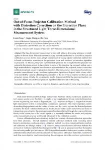
4 Application to NIR spectra of gasoline The method has been applied to predict the octane number based on near infrared (NIR) spectral measurements. The data set contains 60 gasoline samples with specified octane numbers. Samples were measured using diffuse reflectance (R) as log(1/R) from 900 to 1700 nm in 2 nm intervals. So we have N = 60 and m = 401. The data set was divided into five parts for use in a 5-fold cross-validation. To achieve this the octane numbers were sorted in ascending order and numbered successively from 1 to 5 in order to get five sets that cover approximately the same range. We follow Brown (1993, p. 42) and P center all spectra, that is i ai (λj ) = 0; j = 1, . . . , m. The octane numbers are also centered. The mean values of the calibration data is used to center the validation data. For comparison reasons we have applied the well known methods, PCR, PLS, Ridge and LASSO, to the setup described above, i.e. using model (1) without β0 . The optimal model for the methods is chosen by minimizing the root mean squared error of prediction, (RMSEP), based on the 5-fold cross-validation. These values are summarized in Table 1. PCR, PLS and Ridge produce the best results. Finally, Figure 3 show the parameter estimates plotted against their corresponding wavelengths. The estimates are obtained using the tuning-parameters listed in Table 1 together with the full data set. Method PCR PLS Ridge LASSO
Regularization parameter no. of components = 13 no. of components = 7 Pk = 0.002 (|β|)=236.5
RMSEP 0.2333 0.2327 0.2357 0.2779
Table 1: RMSEP-values for the regularization methods.
We now use the model defined by (6) and (8), with b1 (λ), . . . , bk (λ) generated using a cubic B -spline basis with knots placed equidistantly over the range of wavelengths. If
we restrict the number of basis-functions to be less than the number of observations, N , we have a standard linear regression problem which can be solved using ordinary least squares. If we allow the number of basis-functions to exceed the number of observations we can apply PCR, PLS, Ridge or LASSO. The same setup as mentioned earlier is used to find the best model. The approach is straightforward, find the RMSEP-values for a fixed regularization parameter and varying number of basis-functions, now fix the regularization parameter to another value and find new RMSEP-values. This produces a matrix of RMSEP-values; find the smallest RMSEP-value and the corresponding value for the regularization parameter and the P number of basis-functions. For LASSO the optimum is (|θ|)=17.15 and 33 internal knots; Figure 2 indicates the curvature of the RMSEP-surface around the optimum. RMSEP−values for LASSO with Σ(|θ|)=17.15
RMSEP−values for LASSO with 33 internal knots 0.3
1.4 0.28
1.2 1
RMSEP
RMSEP
0.26
0.24
0.8 0.6
0.22 0.4 0.2
0.18 0 10
0.2
1
10 LASSO tuning parameter
2
10
0
0
50 100 Number of knots
150
Figure 2: P The RMSEP-values for LASSO for fixed number of internal knots (left) and fixed value for (|θ|) (right).
The RMSEP-values are listed in Table 2. It is seen that LASSO performs best and that all methods are superior to the methods listed in Table 1. Comparing the best results between Table 1 and 2 results in a 17% reduction in RMSEP-values when using spline functions. The simple OLS-solution results in a 12% reduction. Method OLS PCR PLS Ridge LASSO
Regularization parameter no. of components = 7 no. of components = 7 Pk=0.0008 (|θ|)=17.15
No. of internal knots RMSEP 4 0.2053 4 0.2001 4 0.2012 4 0.2002 33 0.1926
Table 2: RMSEP-values for the regularization methods combined with the spline-method.
Figure 4 show the estimates of β(λ) = B0 (λ)θ. The estimates are obtained using the tuning-parameters listed in Table 2 together with the full data set. For the OLS-solution curves indicating two times the pointwise standard error are also shown (obtained by
disregarding that the number of internal knots are selected by use of cross-validation). For all but LASSO the estimates are quite similar. Comparing the standard error bands of the OLS-solution with the LASSO-solution reveals that LASSO selects basis-functions corresponding to wavelengths for which the OLS-solution is significantly different from zero.
5 Conclusion and discussion An approach to multivariate calibration in which the model is formulated using an integral of an unknown coefficient-function multiplied with the measured spectrum is presented. The unknown function is approximated as a linear combination of some basis functions, whereby estimation is made feasible. A key feature of the method is that the dimension of the resulting model is not dependent on the number of wavelengths at which the spectral measurements are performed. When the number of basis functions is low, standard linear regression techniques can be applied. However, some of the regressors may be collinear when the number of basis functions increase. In this case standard shrinkage methods used in multivariate calibration can be applied. This also opens the possibility of using more basis functions than the number of observations. In an example with 60 near infrared spectra of gasoline, which are used to predict octane numbers, cubic B -spline bases with knots placed equidistantly are used. Compared to standard methods the spline-based methods performs 12% to 17% better in terms of the root mean square of five-fold cross-validated prediction errors (RMSEP). Even the simple linear regression model obtained when using eight basis functions results in a 12% reduction in RMSEP compared to the standard methods. When the number of basis functions are low the knot placement may have large influence; it may move the valleys and peaks (Hastie & Tibshirani 1990, pp. 251-254). To avoid this the smoothing splines solution used by Hastie & Mallows (1993) and Goutis (1998) may be applied. The P -spline approach by Marx & Eilers (1999) provides a mix between these two approaches. All these approaches result in estimates of the coefficient-function which have approximately the same degree of smoothness for all wavelengths for which the spectral measurements are performed. There is no reason to believe that this is desirable. The B -spline/LASSO approach is one solution to the problem just outlined. Another solution would be to use wavelet basis functions together with LASSO. Since wavelets cover a large range of scales and positions, they may be more appropriate than B -splines.
As yet another solution an adaptive knot-placement procedure could be applied together with standard linear regression. It is however not clear how to construct such a procedure. For people using the traditional multivariate calibration techniques the main problem of applying the techniques presented here is the generation of spline bases. In S-PLUS (www.splus.mathsoft.com) and R (www.r-project.org) these can be generated with the build-in functions bs (B -splines) or ns (natural splines). In Matlab (www.mathworks.com) we use bsplval.m by Dr. Graeme A. Chandler, Mathematics Department, The University of Queensland, Australia. A ZIP-archive containing this function can be downloaded as www.maths.uq.edu.au/∼gac/mn309/mfilez.zip and in www.maths.uq.oz.au/∼gac/mn309/bspl.html examples of how to apply it can be found.
References Brown, P. J. (1993), Measurement, Regression, and Calibration, Clarendon Press, Oxford. (ISBN 0198522452). Bruce, A. & Gao, H.-Y. (1996), Applied Wavelet Analysis With S-Plus, Springer-Verlag, Berlin/New York. de Boor, C. (1978), A Practical Guide to Splines, Springer Verlag, Berlin. Goutis, C. (1998), ‘Second-derivative functional regression with applications to near infra-red spectroscopy’, Journal of the Royal Statistical Society, Series B, Methodological 60, 103–114. Hastie, T. J. & Tibshirani, R. J. (1990), Generalized Additive Models, Chapman & Hall, London/New York. Hastie, T. & Mallows, C. (1993), ‘Comment on “A statistical view of some chemometrics regression tools”’, Technometrics 35, 140–143. Marx, B. D. & Eilers, P. H. C. (1999), ‘Generalized linear regression on sampled signals and curves: A P-spline approach’, Technometrics 41(1), 1–13. Osborne, M. R., Presnell, B. & Turlach, B. A. (2000), ‘On the LASSO and its dual’, Journal of Computational and Graphical Statistics 9(2), 319–337.
60 NIR spectra of gasoline
log(1/R)
1.5 1 0.5 0 900
1000
1100
1200
1300 1400 Wavelength (nm)
1500
1600
1700
Parameter estimates, β 5 PCR β
0
−5
−10 900
1000
1100
1200
1300
1400
1500
1600
1700
1000
1100
1200
1300
1400
1500
1600
1700
1000
1100
1200
1300
1400
1500
1600
1700
1100
1200
1300 1400 Wavelength (nm)
1500
1600
1700
5 PLS β
0
−5
−10 900 4 2
Ridge
β
0 −2 −4 −6 900 40 20
LASSO
β
0 −20 −40 −60 900
1000
Figure 3: The 60 NIR spectra, together with the parameter estimates for PCR, PLS, Ridge and LASSO.
Parameter functions,B(λ)θ 6
B(λ)θ
4
Spline−PCR
2 0 −2 −4 −6 900
1000
1100
1200
1300
1400
1500
1600
1700
1100
1200
1300
1400
1500
1600
1700
1100
1200
1300
1400
1500
1600
1700
1100
1200
1300
1400
1500
1600
1700
1100
1200
1300 1400 Wavelength (nm)
1500
1600
1700
6
B(λ)θ
4
Spline−PLS
2 0 −2 −4 −6 900
1000
6
B(λ)θ
4
Spline−Ridge
2 0 −2 −4 −6 900
1000
6
B(λ)θ
4
Spline−OLS +−2stderr
2 0 −2 −4 −6 900
1000
6
B(λ)θ
4
Spline−LASSO
2 0 −2 −4 −6 900
1000
Figure 4: Estimated coefficient-functions using PCR, PLS, Ridge, OLS, and LASSO together with spline bases.