May 31, 2010 - Springer, 2006. [DZLM04] Silvano Dal-Zilio, Denis Lugiez, and Charles Meyssonnier. .... James W. Thatcher and Jesse B. Wright. Generalized ...
A Tree Logic with Graded Paths and Nominals Everardo Bárcenas — Pierre Genevès — Nabil Layaïda — Alan Schmitt
N° 7251 April 2010
apport de recherche
ISRN INRIA/RR--7251--FR+ENG
Knowledge and Data Representation and Management
SN 0249-6399
arXiv:1005.5623v1 [cs.DB] 31 May 2010
INSTITUT NATIONAL DE RECHERCHE EN INFORMATIQUE ET EN AUTOMATIQUE
A Tree Logic with Graded Paths and Nominals Everardo B´arcenas , Pierre Genev`es , Nabil Laya¨ıda , Alan Schmitt Theme : Knowledge and Data Representation and Management ´ Equipes-Projets WAM et SARDES Rapport de recherche n° 7251 — April 2010 — 34 pages
Abstract: Regular tree grammars and regular path expressions constitute core constructs widely used in programming languages and type systems. Nevertheless, there has been little research so far on reasoning frameworks for path expressions where node cardinality constraints occur along a path in a tree. We present a logic capable of expressing deep counting along paths which may include arbitrary recursive forward and backward navigation. The counting extensions can be seen as a generalization of graded modalities that count immediate successor nodes. While the combination of graded modalities, nominals, and inverse modalities yields undecidable logics over graphs, we show that these features can be combined in a tree logic decidable in exponential time. Key-words: Modal Logic, XML, XPath, Schema
Centre de recherche INRIA Grenoble – Rhône-Alpes 655, avenue de l’Europe, 38334 Montbonnot Saint Ismier Téléphone : +33 4 76 61 52 00 — Télécopie +33 4 76 61 52 52
A Tree Logic with Graded Paths and Nominals R´ esum´ e : Ce document introduit une logique d’arbre d´ecidable en temps exponentielle et qui est capable d’exprimer des contraintes de cardinalit´e sur chemins multidirectionnelle Mots-cl´ es : Logique Modal, XML, XPath, Schema
A Tree Logic with Graded Paths and Nominals
1
3
Introduction
A fundamental peculiarity of XML is the description of regular properties. For example, in XML schema languages the content types of element definitions is made through the use of regular expressions. In addition, selecting nodes in such constrained trees is also done by the mean of regular path expressions (`a la XPath). In both cases, it is often interesting to be able to express conditions on the frequency of occurrences of nodes. Even if we consider simple strings, it is well known that some formal languages easily described in English may require voluminous regular expressions. For instance, as pointed in [HJJ+ 95], the language L2a2b of all strings over Σ = {a, b, c} containing at least two occurrences of a and at least two occurrences of b seems to require a large expression, such as: Σ∗ aΣ∗ aΣ∗ bΣ∗ bΣ∗
∪
∪
Σ∗ aΣ∗ bΣ∗ bΣ∗ aΣ∗
∪
∪
Σ bΣ aΣ bΣ aΣ
∪
∗
∗
∗
∗
∗
Σ∗ aΣ∗ bΣ∗ aΣ∗ bΣ∗
Σ∗ bΣ∗ bΣ∗ aΣ∗ aΣ∗
Σ∗ bΣ∗ aΣ∗ aΣ∗ bΣ∗ .
If we added ∩ to the operators for forming regular expressions, then the language {a, b, c} could be expressed more concisely as (Σ∗ aΣ∗ aΣ∗ ) ∩ (Σ∗ bΣ∗ bΣ∗ ). In logical terms, conjunction offers a first dramatic reduction in expression size. If we now consider a formalism equipped with the ability of describing numerical constraints on the frequency of occurrences, we get a second (exponential) reduction in size. For instance, the above expression can be formulated as 20 20 (Σ∗ aΣ∗ )2 ∩ (Σ∗ bΣ∗ )2 . We can even write (Σ∗ aΣ∗ )2 ∩ (Σ∗ bΣ∗ )2 instead of a (much) larger expression. Different extensions of regular expressions with intersection, counting constraints, and interleaving have been recently considered over strings, and for describing content models of sibling nodes in XML type languages [CGS09, GMN08, KT07]. The complexity of the inclusion problem over these different language extensions and their combinations typically ranges from polynomial to exponential space (see [GMN08] for a survey). The main distinction between these works and the work presented here is that we focus on counting nodes located along deep and recursive paths in trees. When considering regular tree languages instead of regular string languages, succinct syntactic sugars such as the ones presented above are even more useful, as branching makes the situation more combinatorial compared to strings. In the case of trees, it is often useful to express cardinality constraints not only on the sequence of children nodes, but also in a particular region of a tree: in a subtree for example. Suppose for instance that we want to define a tree language over Σ where there is no more than 2 “b” nodes. This seems to require a quite
RR n° 7251
A Tree Logic with Graded Paths and Nominals
4
large regular tree type expression such as the one below: xroot → b[xb≤1 ] ∣ c[xb≤2 ] ∣ a[xb≤2 ] xb≤2 → x¬b , b[x¬b ], x¬b , b[x¬b ], x¬b ∣ x¬b , b[xb≤1 ], x¬b ∣ x¬b , a[xb≤2 ], x¬b ∣ x¬b , c[xb≤2 ], x¬b ∣ xb≤1 xb≤1 → x¬b ∣ x¬b , b[x¬b ], x¬b ∣ a[xb≤1 ] ∣ c[xb≤1 ] x¬b → (a[x¬b ] ∣ c[x¬b ])∗ where xroot is the starting non-terminal; x¬b , xb≤1 , xb≤2 are non-terminals; and the bracket notation a[x¬b ] describes a subtree whose root is labeled a and in which there is no b node. More generally, the widely adopted notations for regular tree grammars produce very verbose definitions for properties involving cardinality constraints on the nesting of elements1 . The problem with regular tree (and even string) grammars is that one is forced to fully expand all the patterns of interest using concatenation, union, and Kleene star. Instead, it is often tempting to rely on another kind of (formal) notation that just describes a simple pattern and additional constraints on it. For instance, one could imagine denoting the previous example as follows, where the additional constraint is described using XPath notation: (x→(a[x] ∣ b[x] ∣ c[x])∗ ) ∧ count(/descendant-or-self::b) ≤ 2 Although this kind of counting operators does not increase the expressive power of the regular tree grammars, they can have a drastic impact on succinctness, thus making reasoning over these languages harder (as noticed in [Gel08] in the case of strings). Indeed, reasoning on this kind of extensions without relying on their expansion (in order to avoid syntactic blow-ups) is often tricky [GGM09]. Determining satisfiability, containment, and equivalence over these classes of extended regular expressions typically require involved algorithms with extra-complexity [MS72] compared to plain vanilla regular expressions. In the present paper, we propose a logical notation that happens to be especially appropriate for describing many sorts of cardinality constraints on the frequency of occurrence of nodes in regular tree types. Regular tree types encompass most of XML types (DTDs, XML Schemas, RelaxNGs) used in practice today. XPath is the standard query language for XML documents, and it is an important part of other XML technologies such as XSLT and XQuery. XPath expressions are regular path expressions interpreted as sets of nodes selected from a given context node. In contrast with regular tree types, which only express properties on children nodes, most of the expressive power of XPath comes from the ability to perform multidirectional navigation, that is, XPath expressions are able to express properties involving not only recursive navigation, as 1 This is typically the reason why the standard DTD for XHTML does not syntactically prevent the nesting of anchors, whereas this nesting is actually prohibited in the XHTML standard.
RR n° 7251
A Tree Logic with Graded Paths and Nominals
5
0 1
0 1 2
2 3
3
Figure 1: n−ary to binary trees for descendant nodes for instance, but also backward navigation, as for ancestor nodes. Unfortunately, expressing cardinality restrictions on nodes accessible by recursive multidirectional paths may introduce an extra-exponential cost [GR05, tCM09], or may even lead to undecidable formalisms [tCM09, DL06]. We propose in this paper a decidable framework capable of succinctly express cardinality constraints along deep multidirectional paths. Contribution and Outline We introduce a tree logic with counting operators for expressing arbitrarily deep and recursive counting constraints in Section 2. A sound and complete algorithm for testing satisfiability of logical formulas in exponential time is presented in Section 3. Section 4 shows how the logic and the algorithm can be applied in the XML setting and in particular for the static analysis of XPath expressions and common schemas containing constraints on the frequency of occurrence of nodes. Finally, we review related works in Section 5 before concluding in Section 6.
2
Counting Tree Logic
We first present trees that we consider, and define a notion of trails in trees, before introducing the syntax and semantics of logical formulas.
2.1
Trees
We consider finite trees which are node-labeled and sibling-ordered. Since there is a well-known bijective encoding between n−ary and binary trees, we focus on binary trees without loss of generality. Specifically, we use the encoding represented in Figure 1, where the binary representation preserves the first child of a node and append sibling nodes as second successors. We consider the modalities “▽” and “▷”. The modality “▽” labels the edge between a node and its first child. The modality “▷” labels the edge between a node and its next sibling. We also consider the converse modalities “△” and “◁” that respectively labels the same edges in the reverse direction.
RR n° 7251
A Tree Logic with Graded Paths and Nominals
6
In order to define a simple set theoretic semantics for the logic, we consider trees in a way similar to Kripke structures for modal logics [Var98]. Specifically, we name M = {▽, ▷, △, ◁} the set of modalities. For m ∈ M we denote by m the corresponding inverse modality (▽ = △, ▷ = ◁, △ = ▽, ◁ = ▷). We consider a countable alphabet P of propositions representing names of nodes. A node is labeled with exactly one proposition. A tree can then be seen as a tuple (N, R, L), where: N is a finite set of nodes; R is a partial mapping from N × M to N that restricts the labeling of edges to form a tree structure; and L is a labeling function from N to P .
2.2
Trails
Trails are defined as regular expressions formed by modalities, as follows: α0 ∶∶= m ∣ α0 , α0 ∣ α0 ∣ α0 α ∶∶= α0 ∣ α0⋆ α0
We restrict trails to sequences or repeated subtrails (which contain no repetition) followed by a subtrail (with no repetition). We also disallow trails of the form m, m, which may result in formulas with cycles. The syntactic interpretation of trails corresponds to sets of sequences of modalities (as in the usual semantics of regular expressions). In a given tree, we say that there is a trail α from the node n0 to the node α nk , written n0 Ð→ nk , if and only if there is a sequence of nodes n0 , . . . , nk and a sequence of modalities m1 , . . . , mk that belongs to the syntactic interpretation of the trail α, such that R(nj , mj+1 ) = nj+1 , where j = 0, . . . , k − 1. We say that a path ρ among two nodes belongs to a trail α, written ρ ∈ α, if there exists a sequence of modalities between the nodes that belongs to the interpretation of the trail.
2.3
Syntax of Logical Formulas
The syntax of logical formulas is given in Figure 2, where m ∈ M and k ∈ N. The syntax is shown in negation normal form, which can be reached usual De Morgan rules together with rules given in Figure 3. The fact that the semantic interpretation is preserved even though the smallest fixpoint does not become a greatest fixpoint is a consequence of Lemma 2.1. Defining an equality operator for counting formulas is straightforward. ⟨α⟩=k ψ ≡ ⟨α⟩>(k−1) ψ ∧ ⟨α⟩≤k ψ
if k > 0
⟨α⟩=0 ψ ≡ ⟨α⟩≤0 ψ
2.4
Semantics of Logical Formulas
Formulas are interpreted as sets of nodes in a tree. A model of a formula is a tree, such that the formula denotes a non-empty set of nodes in this tree. A RR n° 7251
A Tree Logic with Graded Paths and Nominals
Φ∋φ
∶∶=
ψ
∣ ∣ ∣ ∣ ∣ ∣ ∣ ∶∶= ∣ ∣ ∣ ∣ ∣ ∣
⊺ ∣ ¬⊺ p ∣ ¬p x φ∨φ φ∧φ ⟨m⟩φ ∣ ¬⟨m⟩⊺ ⟨α⟩≤k ψ ∣ ⟨α⟩>k ψ µx.ψ
7
formula true, false atomic prop (negated) recursion variable disjunction conjunction modality (negated) counting fixpoint operator
⊺ ∣ ¬⊺ p ∣ ¬p x ψ∨ψ ψ∧ψ ⟨m⟩ψ ∣ ¬⟨m⟩⊺ µx.ψ
Figure 2: Syntax of Formulas (in Normal Form).
¬⟨m⟩φ ≡ ¬⟨m⟩⊺ ∨ ⟨m⟩¬φ ¬⟨α⟩≤k ψ ≡ ⟨α⟩>k ψ
¬µx.ψ ≡ µx.¬ψ{x/¬x } ¬⟨α⟩>k ψ ≡ ⟨α⟩≤k ψ
Figure 3: Reduction to Negation Normal Form.
RR n° 7251
A Tree Logic with Graded Paths and Nominals
8
[[⊺]]TV
=
N
[[¬⊺]]TV [[p]]TV [[¬p]]TV [[x]]TV
=
∅
=
{n, L(n) = p}
=
{n, L(n) ≠ p}
=
{n, (n, x) ∈ V }
[[φ1 ∨ φ2 ]]TV [[φ1 ∧ φ2 ]]TV [[⟨m⟩φ]]TV [[¬⟨m⟩⊺]]TV
=
[[φ1 ]]TV ∪ [[φ2 ]]TV
=
[[φ1 ]]TV ∩ [[φ2 ]]TV
=
{n, R(n, m) ∈ [[φ]]TV }
=
{n, R(n, m) undefined}
[[⟨α⟩≤k ψ]]TV
=
[[⟨α⟩>k ψ]]TV
=
[[µx.ψ]]TV
=
{n, ∣{n′ ∈ [[ψ]]TV ∣ n Ð→ n′ }∣ ≤ k} α
{n, ∣{n′ ∈ [[ψ]]TV ∣ n Ð→ n′ }∣ > k} α
′ T ′ ⋂{N , [[ψ]]V [N ′/x ] ⊆ N }
Figure 4: Semantics of Formulas. counting formula ⟨α⟩>k ψ is interpreted as follows: the set of nodes such that there are at least k + 1 nodes satisfying ψ through the trail α. For example, the formula p1 ∧ ⟨▽⟩⟨▷∗ ⟩>5 p2 , denotes p1 nodes with strictly more than 5 children nodes named p2 . In order to present the formal semantics of formulas, we introduce valuations. Given a tree, a valuation V is a binary relation between tree nodes and variables. ′ We write V [N /x ], where N ′ is a subset of the nodes, for the relation denoted by V extended with (n, x) for every n ∈ N ′ . Given a tree T = (N, R, L) and a valuation V , the formal semantics of formulas is given in Figure 4. Intuitively, the formulas are interpreted as sets of nodes in a tree: propositions denote the nodes where they occur; negation is interpreted as set complement; disjunction and conjunction are respectively set union and intersection; the least fixpoint operator performs finite recursive navigation; and the counting operator denotes certain nodes, named the source nodes, such that the nodes, accessible from a single source through a trail, fulfill a cardinality restriction. A formula is said to be satisfiable when its interpretation is not empty.
2.5
Restriction over Formulas
We consider a syntactic restriction over formulas similar to the one in [GLS07]: every formula of the logic must be cycle-free (so that the logic is closed under negation [GLS07]). Intuitively, in a cycle-free formula, fixpoint variables do not occur in the scope of both a modality and its converse. For example, cycle-free trails are trails where both a subtrail and its converse do not occur under the RR n° 7251
A Tree Logic with Graded Paths and Nominals
9
scope of the recursion operator. We do not consider counting formulas under fixpoints nor under counting formulas. Lemma 2.1. Let φ be a cycle-free formula, and T be a tree for which [[φ]]T∅ ≠ ∅. Then there is a finite unfolding φ′ of the fixpoints of φ such that [[φ′ {¬⊺/µx.ψ }]]T∅ = [[φ]]T∅ . Proof. As counting formulas may be replaced by non-counting formulas (with the cost of an exponential blow up), the proof is identical to the one in [GLS07].
2.6
Global Counting Formulas and Nominals
An interesting consequence of the inclusion of backward axes in trails is the ability to reach every node in the tree from a given node of the tree, using the trail (△∣◁)⋆ , (▽∣▷)⋆2 . We can thus select some nodes depending on some global counting property. Consider the following formula, where # stands for one of the comparison operators ≤, >, =. ⟨(△∣◁)⋆ , (▽∣▷)⋆ ⟩#k φ1 Intuitively, this formula considers each node n of the tree, and counts how many nodes in the whole tree satisfy φ1 . It then selects node n if and only if the count is compatible with the comparison considered. This formula thus returns either every node of the tree, or the empty set. It is then easy to restrict the selected nodes to some that satisfy a given formula φ2 , using intersection. ⟨(△∣◁)⋆ , (▽∣▷)⋆ ⟩#k φ1 ∧ φ2 This formula select every node satisfying φ2 if and only if there are #k nodes satisfying φ1 , which we write as follows. φ1 #k Ô⇒ φ2 We can now express existential properties, such as “select all nodes satisfying φ2 if there exists a node satisfying φ1 ”. φ1 > 0 Ô⇒ φ2 We can also express universal properties, such as “select all nodes satisfying φ2 if every node satisfies φ1 ”. (¬φ1 ) ≤ 0 Ô⇒ φ2 Another way to interpret global counting formulas is as a generalization of the so-called nominals in the modal logics community [SV01]. Nominals are special propositions whose interpretation is a singleton (they occur exactly once 2 Note
that this trail is cycle-free.
RR n° 7251
A Tree Logic with Graded Paths and Nominals
10
in the model). They come for free with the logic. A nominal, denoted “@n” in the remaining part of the paper, corresponds to the following global counting formula: ⟨(△∣◁)⋆ , (▽∣▷)⋆ ⟩=1 n where n is a new fresh atomic proposition. Notice that we can also perform a navigation to everywhere in a tree with only fixpoint formulas, hence a nominal can be alternatively written as: @n ≡ n ∧ ¬[descendant(n) ∨ ancestor(n)∨ desc−or−self(siblings(n))∨ desc−or−self(siblings(ancestor(n)))], where:
2.7
descendant(φ)
=
⟨▽⟩µx.φ ∨ ⟨▽⟩x ∨ ⟨▷⟩x
foll−sibling(φ)
=
µx.⟨▷⟩φ ∨ ⟨▷⟩x
prec−sibling(φ)
=
µx.⟨◁⟩φ ∨ ⟨◁⟩x
desc−or−self(φ)
=
µx0 .φ ∨ ⟨▽⟩µx1 .x0 ∨ ⟨▷⟩x1
ancestor(φ)
=
µx.⟨△⟩(φ ∨ x) ∨ ⟨◁⟩x
siblings(φ)
=
foll−sibling(φ) ∨ prec−sibling(φ)
Graded Paths
Graded modalities have been introduced to count immediate successor nodes in graphs [KSV02]. Specifically, graded modalities make it possible to restrict the number of occurrences of immediate successors of a node in a graph by the mean of an explicit constant upper-bound and/or lower-bound. Here we consider trees and extend the “immediate successor” notion to nodes reachable from any regular path, including reverse and recursive navigation. A peculiarity of graded modalities in graphs is that they can be used inside recursive formulas. A similar notion in trees consists in counting immediate children nodes, as performed by the counting formula ⟨▽⟩⟨▷∗ ⟩#k φ, where φ describes the property to be counted. It is then possible to consider occurrences of this counting formula inside a fixpoint operator. This is because this peculiar counting formula can be simply rewritten in terms of plain vanilla logical formulas. For instance, the formula ⟨▽⟩⟨▷∗ ⟩>1 p states the existence of at least two “p” children, and is translated into: ⟨▽⟩µx.(p ∧ ⟨▽⟩µy.p ∨ ⟨▷⟩y) ∨ ⟨▷⟩x The general nesting scheme of this translation can be expressed as follows, where the function ch(⋅) takes such a counting formula as input and returns
RR n° 7251
A Tree Logic with Graded Paths and Nominals
11
its translation: ch(⟨▽⟩⟨▷∗ ⟩>0 φ) =⟨▽⟩µx.φ ∨ ⟨▷⟩x
ch(⟨▽⟩⟨▷∗ ⟩>k+1 φ) =⟨▽⟩µx. (φ ∧ ch(⟨▽⟩⟨▷∗ ⟩>k φ)) ∨ ⟨▷⟩x ch(⟨▽⟩⟨▷∗ ⟩≤k φ) =¬ch(⟨▽⟩⟨▷∗ ⟩>k φ)
We can even apply a recursive version of this transformation in order to rewrite nested counting formulas. In Lemma 3.12, we show the computational cost of the translation does not depend on the size of the formula, but on the nesting level of counting subformulas. The possibility of using an arbitrary fixpoint operator around a given formula allows one to express the “until” operator, proposed for XPath by Marx [Mar05]. Owing to the previous translation, we can combine counting features with the “until” operator and express properties that go beyond the expressive power of the XPath 1.0 standard. For instance, the following formula states that “starting from the current node, until we reach an ancestor named a, every ancestor has at least 3 children named b”: µx. (⟨▽⟩⟨▷∗ ⟩>2 b ∧ µy.⟨△⟩x ∨ ⟨◁⟩y) ∨ a
3
Satisfiability Algorithm
We present a tableau-based algorithm for checking satisfiability of formulas. Given a formula, the algorithm seeks to build a satisfying tree. A satisfying tree is found if and only if the formula is satisfiable, otherwise the algorithm concludes that the formula is unsatisfiable.
3.1
Overview
The algorithm operates in two stages. First, a formula φ is decomposed into a set of subformulas, called the Lean. The Lean gathers all subformulas that are useful for determining the truth status of the initial formula, while eliminating redundancies. For instance, conjunctions and disjunctions are eliminated at this stage, since, if a subformula φ1 holds then one does not need to know the truth status of φ2 in order to determine the truth status of φ1 ∨ φ2 . In fact, the lean (defined in 3.2) only gathers atomic propositions and modal subformulas. The Lean defines a finite number of formulas that can be composed. The set of all these compositions represents the exhaustive search universe in which the algorithm is looking for a satisfying tree. A tree node corresponds to a valuation of the Lean formulas. The second stage of the algorithm consists in a least fixpoint computation that builds every relevant binary tree in a bottom-up manner. At the first step of this stage, all possible leaves are considered. At each further step, the algorithm considers every possible parent node that can be connected with a node of the
RR n° 7251
A Tree Logic with Graded Paths and Nominals
12
previous steps. At each step, built subtrees are checked for consistency: for instance if a formula at a node n involve a forward modality ⟨▽⟩φ′ , then φ′ must be verified at the first child of n. Reciprocally, due to converse modalities, a given node may impose restrictions on its possible parent nodes. The algorithm only considers consistent nodes at each step, meaning that the whole subtree of a given node added at a given step provably satisfies a subformula, except its potential top-level backward modalities that will be taken into account at the next step. At each step, counting formulas are verified. Finally, the algorithm terminates whenever: • either a tree that satisfies the initial formula has been found, and its root does not contain any pending (unproven) backward modality; or • no more parent nodes can be considered (the exploration of the whole search universe is complete): the formula is unsatisfiable. The algorithm is proven sound and complete: φ is satisfiable if and only if a tree in which φ is satisfied at some node is built. Thus either such a tree is built, or φ is not satisfiable.
3.2
Preliminaries
We first annotate every counting formula with a fresh counting proposition c, written ⟨α⟩c#k φ. We first formally define the notions of Lean and nodes. To this end, we first need to extract navigating formulas from counting formulas. nav(x) = x nav(p) = p nav(⊺) = ⊺ nav(c) = c nav(¬p) = ¬p nav(¬⟨m⟩⊺) = ¬⟨m⟩⊺ nav(φ1 ∧ φ2 ) = nav(φ1 ) ∧ nav(φ2 ) nav(φ1 ∨ φ2 ) = nav(φ1 ) ∨ nav(φ2 ) nav(⟨m⟩φ) = ⟨m⟩nav(φ) nav(µx.ψ) = µx.nav(ψ) nav(⟨α⟩c>k ψ) = nav((α), ψ ∧ c) nav(⟨α⟩c≤k ψ) = nav((α), (ψ ∧ c) ∨ (¬ψ ∧ ¬c)) nav((�), ψ) = ψ nav((m), ψ) = ⟨m⟩ψ nav((α1 , α2 ), ψ) = nav((α1 ), nav((α2 ), ψ)) nav((α1 ∣ α2 ), ψ) = nav((α1 ), ψ) ∨ nav((α2 ), ψ) nav((α⋆ ), ψ) = µx.nav(ψ) ∨ nav((α), x)
RR n° 7251
A Tree Logic with Graded Paths and Nominals
13
We define the Fisher-Ladner relation among formulas as follow, where i = 1, 2. Rf l (φ1 ∧ φ2 , φi ),
Rf l (φ1 ∨ φ2 , φi ),
Rf l (µx.φ, φ[µx.φ/x ]),
Rf l (⟨α⟩c#k ψ, nav(⟨α⟩c#k ψ)),
Rf l (⟨m⟩φ, φ). The Fisher-Ladner closure of a formula φ, written F L(φ), is the set defined as follow. F L(φ)0
=
{φ},
F L(φ)i+1
=
F L(φ)i ∪ {φ′ ∣ Rf l (φ′′ , φ′ ), φ′′ ∈ F L(φ)i },
F L(φ)
=
F L(φ)k ,
where k is the smallest integer s.t. F L(φ)k = F L(φ)k+1 . Note that this set is finite: fixpoints are only expanded once. The Lean set of a formula φ includes navigating formulas of the form ⟨m⟩⊺, every navigating formulas of the form ⟨m⟩φ′ from the Fisher-Ladner closure, every proposition occurring in φ, written Pφ , every counting proposition, written C, and an extra proposition that does not occur in φ used to represent other names, written pφ . Lean(φ) = {⟨m⟩⊺} ∪ {⟨m⟩φ′ ∈ F L(φ)} ∪ Pφ ∪ C ∪ {pφ } A φ−node , written nφ , is a non-empty subset of Lean(φ), such that: • exactly one proposition from Pφ ∪ {pφ } is in each φ−node; • when ⟨m⟩φ′ ∈ nφ , then ⟨m⟩⊺ ∈ nφ ; and • both ⟨△⟩⊺ and ⟨◁⟩⊺ cannot be in the same φ−node. The set of φ−nodes is defined as N φ . Intuitively, the formula corresponding to a node nφ is the following. nφ = ⋀ ψ ∧ ψ∈nφ
⋀
ψ∈Lean(φ)∖nφ
¬ψ
When the formula φ under consideration is fixed, we often omit the superscript. A φtree is either the empty tree ∅, or a triple (nφ , Γ1 , Γ2 ) where Γ1 and Γ2 are φtrees. We now turn to the definition of consistency of a φtree. First, we define an entailment relation between a node and a formula in Figure 5. We can now define the consistency relation between nodes of a φtree.
RR n° 7251
A Tree Logic with Graded Paths and Nominals
n ⊢φ ⊺
ψ∈n
ψ ∈/ n
n ⊢φ ψ
n ⊢φ ¬ψ
14
n ⊢φ ψ1
n ⊢φ ψ2
n ⊢φ ψ1 ∧ ψ2
n ⊢φ ψ2
n ⊢φ ψ{µx.ψ/x }
n ⊢φ ψ1 ∨ ψ2
n ⊢φ µx.ψ
n ⊢φ ψ1 n ⊢φ ψ1 ∨ ψ2
Figure 5: Local entailment relation: between nodes and formulas Two nodes n1 and n2 are consistent under modality m ∈ {▽, ▷}, written Rφ (n1 , m) = n2 , iff ∀⟨m⟩ψ ∈ Lean(φ), ⟨m⟩ψ ∈ n1 ⇐⇒ n2 ⊢φ ψ ∀⟨m⟩ψ ∈ Lean(φ), ⟨m⟩ψ ∈ n2 ⇐⇒ n1 ⊢φ ψ Consistency is checked each time a node is added to the tree, ensuring that forward modalities of the node are indeed satisfied by the nodes below, and that pending backward modalities of the node below are consistent with the added node. Note that do not check counting formulas at this point, as they are globally verified in the next step. Upon generation of a finished tree, i.e., a tree with no pending backward modality, one may check whether a node of this tree satisfies φ. To this end, we first define forward navigation in a φtree Γ. Given a path consisting of forward modalities ρ, Γ(ρ) is the node at that path. It is undefined if there is no such node. (n, Γ1 , Γ2 )(�) = n (n, Γ1 , Γ2 )(▽ρ) = Γ1 (ρ) (n, Γ1 , Γ2 )(▷ρ) = Γ2 (ρ) We also allow extending the path with backward modalities if they match the last modality of the path. (n, Γ1 , Γ2 )(ρ ▽ △) = (n, Γ1 , Γ2 )(ρ) (n, Γ1 , Γ2 )(ρ ▷ ◁) = (n, Γ1 , Γ2 )(ρ) Now, we are able to define an entailment relation along paths in φtrees in Figure 6. This relation extends local entailment relation (Figure 5) with checks for counting formulas. Note that the case for fixpoints is contained in the case for formulas with no counting subformula. Note also that ¬ψ in the “less than” case denotes the negation normal form. We conclude these preliminaries by introducing some final notations. The root of a φtree is defined as follows. root(∅) = ∅ root((n, Γ1 , Γ2 )) = n RR n° 7251
A Tree Logic with Graded Paths and Nominals
φ′ does not contain counting formulas ρ ⊢φΓ φ′
Γ(ρ) ⊢φ φ′
15
ρ ⊢φΓ φ1
ρ ⊢φΓ φ2
ρ ⊢φΓ φ1 ∧ φ2
ρ ⊢φΓ φ1
ρ ⊢φΓ φ2
ρ ⊢φΓ φ1 ∨ φ2
ρ ⊢φΓ φ1 ∨ φ2
ρm ⊢φΓ φ′
ρ ⊢φΓ ⟨m⟩φ′
∣{n′ , ρ′ ∈ α ∧ Γ(ρρ′ ) = n′ ∧ n′ ⊢φ ψ ∧ c}∣ > k ρ ⊢φΓ ⟨α⟩c>k ψ ∣{n′ , ρ′ ∈ α ∧ Γ(ρρ′ ) = n′ ∧ n′ ⊢φ ψ ∧ c}∣ ≤ k ∀ρ′ ∈ α, Γ(ρρ′ ) ⊢φ (ψ ∧ c) ∨ (¬ψ ∧ ¬c) ρ ⊢φΓ ⟨α⟩c≤k ψ Figure 6: Global entailment relation (incl. counting formulas) We extend this notion to multiset of trees and write root(ST ) for the multiset of roots of the trees of ST . The multiset of nodes of a tree is defined as follows. nodes(∅) = ∅ nodes((n, Γ1 , Γ2 )) = {n} ∪ nodes(Γ1 ) ∪ nodes(Γ2 ) We also extend this notion to multiset of trees. A φtree Γ satisfies a formula φ, written Γ ⊢ φ, if neither ⟨△⟩⊺ nor ⟨◁⟩⊺ occur in root(Γ), and if there is a path ρ such that Γ(ρ) = n and n ⊢φΓ,ρ φ. A multiset of trees ST satisfies a formula φ, written ST ⊢ φ, when there is a syntactic tree Γ ∈ ST such that Γ ⊢ φ.
3.3
The Algorithm
We are now ready to present the algorithm, which is parameterized by K(φ), the maximum number of occurrences of a given node in a path from the root of the tree to a leaf. It builds consistent candidate trees from the bottom up, and checks at each step if one of the built tree satisfies the formula, returning 1 if it is the case. As the set of nodes from which to build the trees is finite, it eventually stops and returns 0 if no satisfying tree has been found.
RR n° 7251
A Tree Logic with Graded Paths and Nominals
16
Algorithm 1 Check Satisfiability of φ ST ← ∅ repeat AU X ← {(n, Γ1 , Γ2 ) ∣ {we extend the trees} nmax(n, Γ1 , Γ2 ) ≤ K(φ) + 2 {with an available node} for i in ▽, ▷ {and each child is either} Γi = ∅ and ⟨i⟩⊺ ∉ n {an empty tree} or Γi ∈ ST {or a previously built tree} ⟨i⟩⊺ ∈ root(Γi ) {with pending backward modalities} Rφ (n, i) = root(Γi )} {checking consistency} if AU X ⊆ ST then return 0 {No new tree was built} end if ST ← ST ∪ AU X until ST ⊢ φ return 1
K(p) = K(¬p) = K(¬⟨m⟩⊺) = K(⊺) = K(x) = 0 K(φ1 ∧ φ2 ) = K(φ1 ∨ φ2 ) = K(φ1 ) + K(φ2 ) K(⟨m⟩φ) = K(µx.φ) = K(φ) K(⟨α⟩#k ψ) = k + 1 Figure 7: Occurrences bound We now define the auxiliary nmax function as follows, where max is the usual maximum function between integers. nmax(n, Γ1 , Γ2 ) = max(nmax(n, Γ1 ), nmax(n, Γ2 )) nmax(n, (n, Γ1 , Γ2 )) = 1 + nmax(Γ1 , Γ2 )
nmax(n, (n′ , Γ1 , Γ2 )) = nmax(Γ1 , Γ2 )
if n ≠ n′
nmax(n, ∅) = 0 Note a formula µx.φ can be rewritten in an equivalent formula such that x in φ is only present in formulas with the form ⟨m⟩x. With this last observation, we now define the parameter for the number of occurrence of the same node in the tree in Figure 7. Consider for instance the formula φ = p1 ∧⟨▽⟩⟨▷⋆ ⟩>1 p2 . The computed Lean is as follows, where ψ = µx.p2 ∨ ⟨▷⟩x. {p1 , p2 , p3 , ⟨▽⟩⊺, ⟨▷⟩⊺, ⟨△⟩⊺, ⟨◁⟩⊺, ⟨▽⟩ψ, ⟨▷⟩ψ} Proposition p3 represents names other than p1 and p2 . We now compute the bound on nodes: K = 2. RR n° 7251
A Tree Logic with Graded Paths and Nominals
17
p1 p2
▽ ▷ p2
p1
p2
▷
p3 . . . . . . p2
Figure 8: Checking φ = p1 ∧ ⟨▽⟩⟨▷⋆ ⟩>2 p2 After the first step, ST consists of the trees of the form ({pi }, ∅, ∅) and ({pi , ⟨j⟩⊺}, ∅, ∅), with i ∈ {1, 2, 3} and j ∈ {▽, ▷}. At this point the three finished trees in ST are tested and found not to satisfy φ. After the second iteration many trees are created, but the one of interest is the following. T0 = ({p2 , ⟨▷⟩⊺, ⟨△⟩⊺, ⟨▷⟩ψ}, ∅, ({p2 , ⟨◁⟩⊺}, ∅, ∅)) The third iteration yields the tree ({p1 , ⟨▽⟩ψ, ⟨▽⟩⊺}, T0 , ∅), which is found to satisfy φ at path �. As the nodes at every step are different, the limit is not reached. Figure 8 depicts a graphical representation of the example where counted nodes are drawn as thick circles.
3.4
Termination
Proving termination of the algorithm is straightforward, as only a finite number of trees may be built and the algorithm stops as soon as it cannot build a new tree.
3.5
Soundness
If the algorithm terminates with a candidate, we show that the initial formula is satisfiable. Let Γ, ρ the φtree and path such that ρ ⊢φΓ φ. We extract a tree from Γ and show that the interpretation of φ for this tree includes the node at path ρ. We write T (Γ) for the tree (N, R, L) defined as follows. We first rewrite Γ such that each node n is replaced by the path to reach it. path(n, Γ1 , Γ2 ) → (�, path(▽, Γ1 ), path(▷, Γ2 )) path(ρ, (n, Γ1 , Γ2 )) → (ρ, path(ρ▽, Γ1 ), path(ρ▷, Γ2 )) path(ρ, ∅) → ∅ We then define: RR n° 7251
A Tree Logic with Graded Paths and Nominals
18
• N = nodes(path(Γ)); • for every (ρ, Γ1 , Γ2 ) in path(Γ) and i = ▽, ▷, if Γi ≠ ∅ then R(ρ, i) = ρi and R(ρi, i) = ρ; and • for all ρ ∈ N if p ∈ Γ(ρ) then L(ρ) = p. Lemma 3.1. Let ψ a subformula of φ with no counting formula. If Γ(ρ) ⊢φ ψ T (Γ) then we have ρ ∈ [[ψ]]∅ . Proof. We proceed by induction on the lexical ordering of the number of unfolding of ψ that are required for T (Γ), and of the size of the formula. The base cases are ⊺, atomic or counting propositions, and negated forms. T (Γ) These are immediate by definition of [[ψ]]∅ . The cases for disjunction and conjunction are immediate by induction (the formula is smaller). The case for fixpoints is also immediate by induction, as the number of unfoldings required T (Γ) T (Γ) decreases, and as [[µx.ψ]]∅ = [[ψ{µx.ψ/]]∅ . The last case is the presence of a modality ⟨m⟩ψ from the φnode Γ(ρ). In this case we rely on the fact that the nodes Γ(ρm) and Γ(ρ) are consistent to derive ρm ⊢φ ψ. We then conclude by induction. T (Γ)
Theorem 3.2 (Soundness). If ρ ⊢φΓ φ then ρ ∈ [[φ]]∅
Proof. We proceed by induction on the derivation of ρ ⊢φΓ φ. The proof is a consequence of the more general result ρ′ ⊢φΓ φ′ Ô⇒ ρ′ ∈ T (Γ) [[φ′ ]]∅ for any subformula of φ′ , by induction on the derivation of Γ(ρ′ ) ⊢φΓ,ρ ′ ′ φ . If φ has no counting formula, the result is immediate by Lemma 3.1. Most cases are immediate by induction. As concerns the case for counting formulas, each hypothesis n′ ⊢φ ψ∧c has as hypothesis n′ ⊢φ ψ. This is enough to conclude by induction for the “greater than” case. For the “less than” case, every node that is not counted has to satisfy ¬ψ ∧ ¬c, so in particular ¬ψ, and we conclude by induction.
3.6
Completeness
Our proof proceeds in two step. We build a φtree that satisfies the formula, then we proceed to show it is actually built by the algorithm. Assume that formula φ is satisfiable by a tree T . We consider the smallest such tree (i.e., the tree with the fewest number of nodes) and fix n⋆ , a node witnessing satisfiability. We now build a φtree homomorphic to T , called the Lean labeled version of φ, written Γ(T, φ), and defined as follows. First, we annotate counted nodes along with their corresponding counting proposition, yielding a new tree Tc . Starting from n⋆ and by induction on φ, we proceed as follows. For formulas with no counting subformula, including recursion, we stop. For conjunction and disjunction of formulas, we recursively annotate according to both subformulas. For modalities, recursively annotate RR n° 7251
A Tree Logic with Graded Paths and Nominals
19
from the node under the modality. For ⟨α⟩c≤k ψ, we annotate every selected node with the counting proposition corresponding to the formula. For ⟨α⟩c>k ψ, we annotate exactly k + 1 selected nodes. We now extend the semantics of formulas to take into account counting propositions and annotated nodes, written [[⋅]]TVc . The definition is identical to Figure 4, with one addition and two changes. The addition is for counting propositions, which we define as n ∈ [[c]]TVc iff n is annotated by c. The two changes are for counting propositions, which we define as follows, selected only nodes that are annotated. [[⟨α⟩≤k φ′ ]]TVc = {n, ∣{n′ ∈ [[φ′ ]]TVc ∩ [[c]]TVc , n Ð→ n′ }∣ ≤ k} α
[[⟨α⟩>k φ′ ]]TVc = {n, ∣{n′ ∈ [[φ′ ]]TVc ∩ [[c]]TVc , n Ð→ n′ }∣ > k} α
We show that this modification of the semantics does no change the satisfiability of the formula. Lemma 3.3. We have n⋆ ∈ [[φ]]T∅c . Proof. We proceed by recursion on the derivation n⋆ ∈ [[φ]]T∅ . The cases where no counting formula is involved, thus including fixpoints, are immediate, as the selected nodes are identical. The disjunction, conjunction, and modality cases are also immediate by induction. The interesting cases are the counting formulas. For ⟨α⟩c>k ψ, as there are exactly k+1 nodes annotated, the property is true by induction. For ⟨α⟩c≤k ψ, we rely on the fact that every counted node is annotated. We conclude by remarking that ψ does not contain a counting formula, thus we have [[ψ]]TVc = [[ψ]]TV and [[¬ψ]]TVc = [[¬ψ]]TV . To every node n, we associate nφ , a subset of formulas of the Lean selecting the node. nφ = {φ0 ∣ n ∈ [[φ0 ]]T∅ , φ0 ∈ Lean(φ)} Note that this is a φ-node as it contains one and exactly one proposition, and if it includes a modal formula ⟨m⟩ψ, then it also includes ⟨m⟩⊺. The tree Γ(T, φ) is then built homomorphically to T . In the remainder of this section, we write Γ for Γ(T, φ). We first check that Γ is consistent, starting with local consistency. In the following, we say a formula ψ is induced by the lean of φ, written . ψ ∈ Lean(φ), if it consists of the conjunction and disjunction of formulas from the lean as defined in Figure 9. Lemma 3.4. Let ⟨m⟩ψ be a formula in Lean(φ), and let. ψ ′ be ψ after unfolding its fixpoint formulas not under modalities. We have ψ ′ ∈ Lean(φ). .
Proof. By definition of the lean and of the ∈ relation. Lemma 3.5. Let ψ be a formula induced by Lean(φ). We have n ∈ [[ψ]]T∅c if and only if nφ ⊢φ ψ. RR n° 7251
A Tree Logic with Graded Paths and Nominals
ψ ∈ Lean(φ) .
.
ψ1 ∈ Lean(φ)
ψ ∈ Lean(φ) .
ψ1 ∈ Lean(φ)
20
.
.
ψ1 ∧ ψ2 ∈ Lean(φ)
.
.
ψ2 ∈ Lean(φ)
ψ1 ∨ ψ2 ∈ Lean(φ)
ψ2 ∈ Lean(φ)
.
ψ ∈ (Pφ ∪ ⟨m⟩⊺ ∪ C)
⊺ ∈ Lean(φ)
.
¬ψ ∈ Lean(φ)
Figure 9: Formula induced by a lean Proof. We proceed by induction on ψ. The base cases (the formula is in the φ-node or is a negation of a lean formula not in the φ-node) hold by definition of nφ . The inductive cases are straightforward as these formulas only contain fixpoints under modalities. Lemma 3.6. Let n1 and n2 such that R(n1 , m) = n2 with m ∈ {▽, ▷}. We have Rφ (nφ1 , m) = nφ2 . Proof. Let ⟨m⟩ψ be a formula in Lean(φ). We show that ⟨m⟩ψ ∈ nφ1 ⇐⇒ nφ2 ⊢φ ψ. We have ⟨m⟩ψ ∈ nφ1 if and only if n1 ∈ [[⟨m⟩ψ]]T∅c by definition of nφ1 , which in turn holds if and only if n2 = R(n1 , m) ∈ [[ψ]]T∅c . We now consider ψ ′ which is ψ after unfolding its fixpoint formulas not under modalities. We have [[ψ ′ ]]T∅c = [[ψ]]T∅c and we conclude by Lemmas 3.4 and 3.5. We now turn to global consistency, taking counting formulas into account. Lemma 3.7. Let φs be a subformula of φ, and ρ be a path from the root in T such that T (ρ) ∈ [[φs ]]T∅c . We then have ρ ⊢φΓ φs . Proof. We proceed by induction on φs . If φs does not contain any counting formula, we consider φ′s which is φs ofter unfolding its fixpoint formulas not under modalities. We have [[φ′s ]]T∅c = [[φs ]]T∅c ′ . and φs ∈ Lean(φ). We conclude by Lemma 3.5. For most inductive cases, the proof is immediate by induction, as the formula size decreases. For ⟨α⟩c>k ψ, we have by induction form every counted node Γ(ρρ′ ) ⊢φ ψ and Γ(ρρ′ ) ⊢φ c. We conclude by the conjunction rule and by the counting rule of Figure 6. For ⟨α⟩c≤k ψ, we proceed as above for the counted nodes. For the nodes that are not counted, have [[¬ψ]]TVc = [[¬ψ]]TV and by soundness, we have Γ(ρρ′ ) ⊢φ ¬ψ. We conclude by remarking that the node is not annotated by c, hence Γ(ρρ′ ) ⊢φ ¬c. We now need to show that the φtree Γ is actually built by the algorithm. The proof that it is the case follows closely the one from [GLS07], with a crucial exception: we need to make sure there are enough instances of each formula.
RR n° 7251
A Tree Logic with Graded Paths and Nominals
21
Indeed, in [GLS07], the algorithm uses a φtype (a subset of Lean(φ)) at most once on each branch from the root to a leaf of the built tree. This yields a simple condition to stop the algorithm and conclude the formula is unsatisfiable. However, in the presence of counting formulas, a given φtype may occur more than once on a branch. To maintain the termination of the algorithm, we bound the number of identical φtype that may be needed by K(φ) as defined in Figure 7. We now check that this bound is sufficient to build a tree for any satisfiable formula. We recall that φ is a satisfiable formula and T is a smallest tree such that φ is satisfied, and n⋆ is a witness of satisfiability. We proceed in two steps: first we show that counted nodes (with counted propositions) imply a bound on the number of identical φtypes on a branch for a smallest tree. Second, we show that this minimal marking is bound by K(φ). In the following, we call counted nodes and node n⋆ annotations. We now define the projection of an annotation on a path. Let ρ be a path from the root of the tree to a leaf. An annotation projects on ρ at ρ1 if ρ = ρ1 ρ2 , the annotation is at ρ1 ρm , and ρ2 shares no prefix with ρm . Lemma 3.8. Let Γ′ be the annotated tree, ρ a path from the root of the tree to a leaf, n1 and n2 two distinct nodes of ρ such that nφ1 = nφ2 . Then either annotations projects both on ρ at n1 and n2 , or an annotation projects strictly between n1 and n2 . Proof. We proceed by contradiction: we assume there is no annotation that projects between n1 and n2 and at most one of them has an annotation that projects on it. Without loss of generality, we assume that n2 is below n1 in the tree. Assume neither n1 nor n2 is annotated (through projection). We show that the tree where R(n1 , ▽) ← R(n2 , ▽) and R(n1 , ▷) ← R(n2 , ▷) still satisfies φ at n, a contradiction since this tree is strictly smaller. Let Ts be this smaller tree, Γs the corresponding φtree, and for every path ρ of Γ, let ρs be the potentially shorter path if it exists (i.e., if it was not removed when pruning the tree). More precisely, let ρ1 be the path to n1 and ρ1 ρ2 be the path to n2 . If ρ′ = ρ′1 ρ′3 where ρ′1 is a prefix of ρ1 and the paths are disjoint from there, then Γs (ρ′ ) = Γ(ρ′ ). If ρ′ = ρ1 ρ2 ρ3 , then Γs (ρ1 ρ3 ) = Γ(ρ′ ). First, as there was no annotation projected, n is still part of this tree at a path ρs . We show that we have ρs ⊢φΓs φ by induction on the derivation ρ ⊢φΓ φ. Let ρ′ ⊢φΓ φ′ in the derivation, assuming that ρ′s is defined. The case where φ′ does not mention any counting formula is trivial: Γ(ρ′ ) = Γs (ρ′s ) thus local entailment is immediate. Conjunction and disjunction are also immediate by induction. For the modality case, we first need to prove an additional property. If ρ′ ⊢φΓ ⟨m⟩φ′ and φ′ contains a counting formula, then ρ′ m is either a prefix of ρ1 followed by a disjoint path, or it includes ρ1 ρ2 . We prove this property by contradiction. The formula ⟨m⟩φ′ is both in Γ(ρ1 ) and in Γ(ρ1 ρ2 ). We consider the outermost counting formula in φ′ which we write φ′c . It presence
RR n° 7251
A Tree Logic with Graded Paths and Nominals
22
implies the occurrence of a counting proposition c in the formula. Since counting propositions are distinct for distinct syntactic occurrences of a formula, this implies that the corresponding counting proposition is either under a fixpoint (which is impossible), or under an enclosing counting formula, which is also impossible. We thus have a contradiction We now turn to the counting case ⟨α⟩c#k ψ. We say that a path does not cross over when this path does not contain n1 nor n2 . For nodes that are reached using paths that do not cross over, we conclude by induction that they are also counted. We now show that the remaining nodes for which a crossover happened are also reached. Without loss of generality, assume that ρ′ is a prefix of ρ1 (the counting formula is in the “top” part of the tree), and let ρn be the path from the counting formula to the counted node (ρn is an instance of the trail α). This path is of the shape ρ′1 ρ2 ρc , with ρ1 = ρ′ ρ′1 . We now show that the path ρ′1 ρc is an instance of α if and only if ρn is, thus the same node is still counted. Recall that α is of the shape α1 , . . . , αn , αn+1 where α1 to αn are of the form αr⋆ and where αn+1 does not contain a repeated trail. We say that a prefix ρp of a path ρ stops at i if there is a suffix ρs such that ρp ρs is still a prefix of ρ, if ρp ρs ∈ α1 , . . . , αi , and if there is no shorter suffix ρ′s and j such that ρp ρ′s ∈ α1 , . . . , αj . (Intuitively, αi is the trail being used when matching the end of ρp .) Note that i may not be unique as a path may be matched in different ways by a trail. We now show that there are i ≤ j ≤ n such that both ρ′1 stops at i and ρ′1 ρ2 stop at j. We thus show that j cannot be n + 1. Recall that αn+1 does not contain a repeated subtrail. If nφ2 does not contain the counted proposition c (which may happen in the case of a “less than” counting where the target is not counted), then neither does nφ1 , which is a contradiction to the fact that αi, . . . , αn+1 is not empty (in that case the counted proposition is necessarily mentioned). Thus nφ2 contain formulas without a fixpoint (as the trail is not repeated) mentioning c. Consider the largest such formula. By an induction on the path ρ2 , we build a strictly larger formula that occurs in nφ1 . This a contradiction to the hypothesis that nφ1 = nφ2 . We now consider the suffixes ρ1s and ρ2s computed when stating that the paths stop at i and j. These suffixes correspond to the path matching the end of αi and αj , respectively (before the next iteration or switching to the next formula). They have matching formulas in nφ1 and nφ2 . As the formulas are present in both nodes, then the remainder of the paths (ρ2 ρc and ρc ) are instances of (ρ1s ∣ρ2s )αi . . . αn+1 , thus ρ′1 ρc is an instance of α if and only if ρn is. In the case of “greater than” counting, we conclude immediately by induction as the same nodes are selected (thus there are enough). In the case of “less than”, we need to check that no new node is counted in the smaller tree. Assume it is not the case for the formula ⟨α⟩≤k ψ, thus there is a path ρn ∈ α to a node satisfying ψ. As the same node can be reached in Γ, and as we have Γ(ρ′ ρn ) ⊢φ ¬ψ by induction, we have a contradiction. This concludes the proof when neither n1 nor n2 is annotated. The proof is identical when n2 is annotated. If n1 is annotated, we look at the first
RR n° 7251
A Tree Logic with Graded Paths and Nominals
23
modality between n1 and n2 . If it is a ▽, then we build the smaller tree by doing R(n1 , ▽) ← R(n2 , ▽) (we remove the ▷ subtree from n2 instead of n1 ). Symmetrically, if the first modality is a ▷, we consider R(n1 , ▷) ← R(n2 , ▷) as smaller tree. The rest of the proof proceeds as above. Theorem 3.9 (Completeness). If φ is satisfiable, then a satisfying tree is built. Proof. The proof proceeds as in [GLS07], we only need to check there are enough copies of each node to build every path. Let ρ be a path from the root of the tree to the leaves. By Lemma 3.8, there are at most n+1 identical nodes in this path, where n is the number of marks. The number of marks is c + 1 where c is the number of counted nodes. We show by an immediate induction on the formula φ that c is bound by K(φ) as defined in Figure 7. We conclude by remarking that K(φ) + 2 is the number of identical nodes we allow in the algorithm.
3.7
Complexity
We now show that the complexity of the satisfiability algorithm is exponential time w.r.t. the formula size. This is achieved in two steps: we first show that the Lean size is linear w.r.t. the formula size, then we show that the algorithm has a single exponential complexity w.r.t. to the Lean size. Lemma 3.10. The Lean size is linear in terms of the original formula size. Proof Sketch. It was shown in [GLS07] that the Lean size of non counting formulas is linear with respect to the formula size. We now describe the case for counting formulas. Note that each counting formula introduces only one new counting proposition in the Lean. A first duplication of formulas is considered in the construction of the Lean for ”less than” counting formulas. Both, the formula witnessing the counted nodes and its negation are considered. Furthermore, another duplication is introduced for counting formulas of the form ⟨α1 ∣α2 ⟩#k φ. Each of these duplications only doubles the size of the Lean. Hence, the Lean size remains linear w.r.t to the original formula size. Theorem 3.11. The satisfiability algorithm for the logic is decidable in time 2O(n) , where n is the Lean size. Proof Sketch. The cardinality of nodes set is 2n . The number of occurrences of each node in the tree is bounded by K(φ) ≤ k ∗ m, where k is the greatest constant occurring in the counting formulas and m is the number of counting subformulas. Hence the number of steps in the algorithm is bounded by 2n ∗k∗m. As for the functions at each step, nmax is a single traversal to the tree. Since the entailment relation involved in the definition of Rφ is only local, Rφ is performed in linear time. The number of choices to form trees (triples) at each step is restricted by 3 ∗ (2n ∗ k ∗ m).
RR n° 7251
A Tree Logic with Graded Paths and Nominals
24
The global entailment relation involves four exponential time traversals: the number of trees, the number of nodes at each tree, the number of traversals for the entailment relation of counting formulas, and the cost of each of such traversals. Hence it takes no more than 4 ∗ (2n ∗ k) time. Theorem 3.11 states the complexity for the logic defined in Figure 2. We now state that the same complexity upper-bound holds if we additionally consider counting formulas of the form ⟨▽⟩⟨▷∗ ⟩#k φ in the scope of a fixpoint operator (as presented in Section 2.7). Lemma 3.12. Given a formula φ where counting subformulas ψ only count children nodes, if every counting subformula ψ is replaced by the equivalent fixpoint formula ch(ψ) in φ, φ[ch(ψ)/ψ ], then Lean(φ[ch(ψ)/ψ ]) ≤ Lean(φ) ∗ k l , where k is greatest numerical constraint of the counting subformulas, and l is the greatest level nesting of counting subformulas. Proof Sketch. It is proven by induction on the structure of φ, and in the case of counting formulas, another induction is done on the numerical constraint. Corollary 3.13. The logic supporting counting formulas only on children in the l scope of fixpoint formulas or another counting formula is decidable in 2O(n∗k ) , where k is the greatest cardinality constraint and l is the greatest nesting level of counting formulas. Proof. Immediate from Theorem 3.11 and Lemma 3.12.
4
Application to XML Trees
4.1
XPath Expressions
XPath [CD99] was introduced as part of the W3C XSLT transformation language to have a non-XML format for selecting nodes and computing values from an XML document (see [GLS07] for a formal presentation of XPath). Since then XPath has become part of several other standards, in particular it forms the “navigation subset” of the XQuery language. In their simplest form XPath expressions look like “directory navigation paths”. For example, the XPath /company/personnel/employee navigates from the root of a document through the top-level “company” node to its “personnel” child nodes and on to its “employee” child nodes. The result of the evaluation of the entire expression is the set of all the “employee” nodes that can be reached in this manner. At each step in the navigation, the selected nodes for that step can be filtered with a test. Of special interest to us are the predicates that test node’s count or the selected node’s position in the previous step’s selection. For example, if we ask for RR n° 7251
A Tree Logic with Graded Paths and Nominals
25
/company/personnel/employee[position()=2] then the result is all employee nodes that are the second employee node among the employee child nodes of each personnel node selected by the previous step. XPath also makes it possible to combine the capability of searching along “axes” other than the shown “children of” with counting constraints. For example, if we ask for /company[count(descendant::employee∣≥∣5] This expression selects the children nodes named “a” provided they have more than 5 descendants which (1) are named “b” and (2) whose parent is named “c”. The logical formula denoting the set of children nodes named “a” is: ψ = a ∧ ⟨◁∗ , △⟩⊺ RR n° 7251
A Tree Logic with Graded Paths and Nominals
28
The logical translation of the above XPath expression is: ψ ∧ ⟨▽⟩⟨(▽∣▷)⋆ ⟩>5 (b ∧ µx.⟨△⟩c ∨ ⟨◁⟩x) This formula holds for nodes selected by the XPath expression. A correspondence between the main XPath axes over unranked trees and modal formulas over binary trees is given in Figure 13. In this figure, each logical formula holds for nodes selected by the corresponding XPath axis from a context γ. Path γ/self::* γ/child::* γ/parent::* γ/descendant::* γ/ancestor::* γ/following-sibling::* γ/preceding-sibling::*
Logical formula γ ⟨◁∗ , △⟩γ ⟨▽⟩⟨▷∗ ⟩γ ⟨(◁ ∣ △)∗ , △⟩γ ⟨▽⟩⟨(▽ ∣ ▷)∗ ⟩γ ⟨◁⟩⟨◁∗ ⟩γ ⟨▷⟩⟨▷∗ ⟩γ
Figure 13: XPath axes as modalities over binary trees. Let consider another example (XPath expression e1 ): child::a/child::b[count(child::e/descendant::h])>3] Starting from a given context in a tree, this XPath expression navigates to children nodes named “a” and selects their children named “b”. Finally, it retains only those “b” nodes for which the qualifier between brackets holds. The first path can be translated in the logic as follows: ϑ = b ∧ µx.⟨△⟩(a ∧ µx′ .⟨△⟩⊺ ∨ ⟨◁⟩x′ ) ∨ ⟨△⟩x This example requires a more sophisticated translation in the logic. This is because it makes implicit that “e” nodes (whose existence is simply tested for counting purposes) must be children of selected “b” nodes. The translation of the full aforementioned XPath expression is as follows: ϑ ∧ @n ∧ ⟨(△ ∣ ◁)∗ , (▽ ∣ ▷)∗ ⟩>3 η where @n is a new fresh nominal used to mark a “b” node which is filtered by the qualifier and the formula η describes the counted “h” nodes: η = h ∧ µx.⟨△⟩(e ∧ µx′ .⟨△⟩@n ∨ ⟨◁⟩x′ ) ∨ ⟨◁⟩x ∨ ⟨△⟩x Intuitively, the general idea behind the translation is to first translate the leading path, use a fresh nominal for marking a node which is filtered, then find at least “3” instances of “h” nodes from which we can reach back the marked node via the inverse path of the counting formula.
RR n° 7251
A Tree Logic with Graded Paths and Nominals
29
Since trails make it possible to navigate but not to test properties (like existence of labels), we test for labels in the counted formula η and we use a general navigation (△ ∣ ◁)∗ , (▽ ∣ ▷)∗ to look for counted nodes everywhere in the tree. Introducing the nominal is necessary to bind the context properly (without loss of information). Indeed, the XPath expression e1 makes implicit that a “e” node must be a child of a “b” node selected by the outer path. Using a nominal, we restore this property by connecting the counted nodes to the initial single context node. Lemma 4.1. The translation of Core XPath expressions with counting constraints into the logic is linear. It is proven by structural induction in a similar manner to [GLS07] (in which the translation is proven for expressions without counting constraints). For counting formulas, the use of nominals and the general (constant-size) counting trail make it possible to avoid duplication of trails so that the translation remains linear. Corollary 4.2. The equivalence problem for expressions of the form: PathExpr[count(PathExpr′ )#k] where # ∈ {≤, >, =} and k is a constant, is decidable. More specifically, the equivalence problem can be decided in exponential time in terms of the expression size and the highest nesting level of counting formulas.
4.2
Regular Tree Languages with Cardinality Constraints
Regular tree grammars capture most of the schemas in use today [MLMK05]. The logic can express all regular tree languages (it is easy to prove that regular expression types in the manner of e.g., [HVP05] can be linearly translated into the logic: see [GLS07]). In practice, schema languages often provide shorthands for expressing cardinality constraints on node occurrences. XML Schema notably offers two attributes minOccurs and maxOccurs for this purpose. For instance, the following XML schema definition:
is a notation that restricts the number of occurrences of “b” nodes to be at least 4 and at most 9, as children of “a” nodes. The goal here is to have a succinct notation for expressing regular languages which could otherwise be
RR n° 7251
A Tree Logic with Graded Paths and Nominals
30
exponentially large if written with usual regular expression operators. The above regular requirement can be translated as the formula: φ ∧ ⟨▽⟩(⟨▷⋆ ⟩>3 b ∧ ⟨▷⋆ ⟩≤9 b) where φ corresponds to the regular tree type a[b∗ ] as follows: φ = (a ∧ (¬⟨▽⟩⊺ ∨ ⟨▽⟩ψ)) ∧ ¬⟨▷⟩⊺ ψ = µx. (b ∧ ¬⟨▽⟩⊺ ∧ ¬⟨▷⟩⊺) ∨ (b ∧ ¬⟨▽⟩⊺ ∧ ⟨▷⟩x) This example only involves counting over children nodes. The logic allows counting through more general trails, and in particular arbitrarily deep trails. Trails corresponding to the XPath axes “preceding, ancestor, following” can be used to constrain the context of a schema. The “descendant” trail can be used to specify additional constraints over the subtree defined by a given schema. For instance, suppose we want to forbid webpages containing nested anchors “a” (whose interpretation makes no sense for web browsers). We can build the logical formula f which is the conjunction of a considered schema for webpages (e.g. XHTML) with the formula a/descendant::a in XPath notation. Nested anchors are forbidden by the considered schema iff f is unsatisfiable. As another example, suppose we want paragraph nodes (“p” nodes) not to be nested inside more than 3 unordered lists (“ul” nodes), regardless of the schema defining the context. One may check for the unsatisfiability of the following formula: p ∧ ⟨(△∣◁)⋆ , △⟩>3 ul
5
Related Work
Counting over graphs The µ-calculus is a propositional modal logic augmented with least and greatest fixpoint operators [Koz82]. Kupferman, Sattler and Vardi study a µ-calculus with graded modalities where one can express, e.g., that a node has at least n successors satisfying a certain property [KSV02]. The modalities are limited in scope since they only count children of a given node. The µ-calculus has been recently extended with inverse modalities [Var98], nominals [SV01], and graded modalities [KSV02]. If only two of the above constructs are considered, satisfiability of the enriched calculus is EXPTIMEcomplete [BLMV06]. However, if all of the above constructs are considered simultaneously, the calculus becomes undecidable [BLMV06]. Hopefully, this undecidability result for the case of graphs does not preclude decidable tree logics combining such features. Counting over trees The notion of Presburger Automata for trees, combining both regular constraints on the children of nodes and numerical constraints given by Presburger formulas, has independently been introduced by Dal Zilio and Lugiez [DZLM04] and Seidl et al. [SSMH04]. Specifically, Dal Zilio and RR n° 7251
A Tree Logic with Graded Paths and Nominals
31
Lugiez [DZLM04] propose a modal logic for unordered trees called Sheaves logic. This logic allows to impose certain arithmetical constraints on children nodes but lacks recursion (i.e., fixpoint operators) and inverse navigation. Dal Zilio and Lugiez consider the satisfiability and the membership problems. Demri and Lugiez [DL06] showed by means of an automata-free decision procedure that this logic is only PSPACE-complete. Restrictions like p1 nodes have no more “children” than p2 nodes, are expressible by this approach. Seidl et al. [SSMH04] introduce a fixpoint Presburger logic, which, in addition to numerical constraints on children nodes, also supports recursive forward navigation. For example, expressions like the descendants of p1 nodes have no more “children” than the number of children of descendants of p2 nodes are allowed. This means that constraints can be imposed on sibling nodes (even if they are deep in the tree) by forward recursive navigation but not on distant nodes which are not siblings. Compared to the work presented here, neither of the two previous approaches can support constraints like there are more than 5 ancestors of “p” nodes. Furthermore, due to the lack of backward navigation, the works found in [DZLM04, SSMH04, DL06] are not suited for succinctly capturing XPath expressions. Indeed, it is well-known that expressions with backward modalities are exponentially more succinct than their forward-only counterparts [OMFB02, GR05]. There is poor hope to push the decidability envelope much further for counting constraints. Indeed, it is known from [KR03, DL06, tCM09] that the equivalence problem is undecidable for XPath expressions with counting operators of the form: • PathExpr1 [count(PathExpr2 ) = count(PathExpr3 )], or • PathExpr1 [position() = count(PathExpr2 )]. This is the reason why logical frameworks that allow comparisons between counting operators limit counting by restricting the PathExpr to immediate children nodes [DZLM04, SSMH04]. In this paper, we chose a different tradeoff: comparisons are restricted to constants but at the same time comparisons along more general paths are permitted.
6
Conclusion
We introduced a modal logic of trees equipped with (1) converse modalities, which allow to succinctly express forward and backward navigation, (2) a least fixpoint operator for recursion, and (3) cardinality constraint operators for expressing numerical occurrence constraints on tree nodes satisfying some regular properties. A sound and complete algorithm is presented for testing satisfiability of logical formulas. This result is surprising since the corresponding logic for graphs is undecidable [BLMV06]. The decision procedure for the logic is exponential time w.r.t. to the formula size. The logic captures regular tree languages with cardinality restrictions, as RR n° 7251
A Tree Logic with Graded Paths and Nominals
32
well as the navigational fragment of XPath equipped with counting features. Similarly to backward modalities, numerical constraints do not extend the logical expressivity beyond regular tree languages. Nevertheless they enhance the succinctness of the formalism as they provide useful shorthands for otherwise exponentially large formulas. This makes it possible to extend static analysis to a larger set of XPath and XML schema features in a more efficient way. We believe the field of application of this logic may go beyond the XML setting. For example, in verification of linked data structures [ZKR08, HIV06] reasoning on tree structures with indepth cardinality constraints seems a major issue. Our result may help building solvers that are attractive alternatives to those based on non-elementary logics such as SkS [TW68], like, e.g., Mona [KM01].
References [BLMV06] Piero Bonatti, Carsten Lutz, Aniello Murano, and Moshe Vardi. The complexity of enriched µ-calculi. In Michele Bugliesi, Bart Preneel, Vladimiro Sassone, and Ingo Wegener, editors, ICALP, volume 4052 of Lecture Notes in Computer Science, pages 540–551. Springer-Verlag, 2006. [CD99]
J. Clark and S. DeRose. XML path language (XPath) version 1.0. W3C recommendation, November 1999. http://www.w3.org/TR/1999/REC-xpath-19991116.
[CGS09]
Dario Colazzo, Giorgio Ghelli, and Carlo Sartiani. Efficient asymmetric inclusion between regular expression types. In ICDT ’09: Proceedings of the 12th International Conference on Database Theory, pages 174–182, New York, NY, USA, 2009. ACM.
[DL06]
S. Demri and D. Lugiez. Presburger modal logic is PSPACEComplete. In U. Furbach and N. Shankar, editors, IJCAR, volume 4130 of Lecture Notes in Computer Science, pages 541–556. Springer, 2006.
[DZLM04] Silvano Dal-Zilio, Denis Lugiez, and Charles Meyssonnier. A logic you can count on. In Neil D. Jones and Xavier Leroy, editors, POPL, pages 135–146. ACM, 2004. [Gel08]
Wouter Gelade. Succinctness of regular expressions with interleaving, intersection and counting. In Edward Ochmanski and Jerzy Tyszkiewicz, editors, MFCS, volume 5162 of Lecture Notes in Computer Science, pages 363–374. Springer, 2008.
[GGM09]
Wouter Gelade, Marc Gyssens, and Wim Martens. Regular expressions with counting: Weak versus strong determinism. In Rastislav Kr´ alovic and Damian Niwinski, editors, MFCS, volume 5734 of Lecture Notes in Computer Science, pages 369–381. Springer, 2009.
RR n° 7251
A Tree Logic with Graded Paths and Nominals
33
[GLS07]
P. Genev`es, N. Laya¨ıda, and A. Schmitt. Efficient static analysis of XML paths and types. In PLDI, pages 342–351, New York, NY, USA, 2007. ACM Press.
[GMN08]
Wouter Gelade, Wim Martens, and Frank Neven. Optimizing schema languages for xml: Numerical constraints and interleaving. SIAM J. Comput., 38(5):2021–2043, 2008.
[GR05]
Pierre Genev`es and Kristoffer Høgsbro Rose. Compiling XPath for streaming access policy. In Anthony Wiley and Peter R. King, editors, DocEng, pages 52–54. ACM, 2005.
[HIV06]
Peter Habermehl, Radu Iosif, and Tom´as Vojnar. Automata-based verification of programs with tree updates. In Holger Hermanns and Jens Palsberg, editors, TACAS, volume 3920 of Lecture Notes in Computer Science. Springer, 2006.
[HJJ+ 95]
J.G. Henriksen, J. Jensen, M. Jørgensen, N. Klarlund, B. Paige, T. Rauhe, and A. Sandholm. Mona: Monadic second-order logic in practice. In Tools and Algorithms for the Construction and Analysis of Systems, First International Workshop, TACAS ’95, LNCS 1019, 1995.
[HVP05]
H. Hosoya, J. Vouillon, and B. C. Pierce. Regular expression types for XML. ACM Trans. Program. Lang. Syst., 27(1):46–90, 2005.
[KM01]
Nils Klarlund and Anders Møller. MONA Version 1.4 User Manual. BRICS Notes Series NS-01-1, Department of Computer Science, University of Aarhus, January 2001.
[Koz82]
D. Kozen. Results on the propositional µ-Calculus. In M. Nielsen and E. M. Schmidt, editors, ICALP, volume 140 of Lecture Notes in Computer Science, pages 348–359. Springer, 1982.
[KR03]
F. Klaedtke and H. Rueß. Monadic second-order logics with cardinalities. In J. C. M. Baeten, J. K. Lenstra, J. Parrow, and G. J. Woeginger, editors, ICALP, volume 2719 of Lecture Notes in Computer Science, pages 681–696. Springer, 2003.
[KSV02]
O. Kupferman, U. Sattler, and M. Y. Vardi. The complexity of the graded µ-calculus. In A. Voronkov, editor, CADE, volume 2392 of Lecture Notes in Computer Science, pages 423–437. Springer, 2002.
[KT07]
Pekka Kilpelinen and Rauno Tuhkanen. One-unambiguity of regular expressions with numeric occurrence indicators. Information and Computation, 205(6):890 – 916, 2007.
[Mar05]
Maarten Marx. Conditional xpath. ACM Trans. Database Syst., 30(4):929–959, 2005.
RR n° 7251
A Tree Logic with Graded Paths and Nominals
34
[MLMK05] M. Murata, D. Lee, M. Mani, and K. Kawaguchi. Taxonomy of XML schema languages using formal language theory. ACM Trans. Internet Techn., 5(4):660–704, 2005. [MS72]
Albert R. Meyer and Larry J. Stockmeyer. The equivalence problem for regular expressions with squaring requires exponential space. In FOCS, pages 125–129. IEEE, 1972.
[OMFB02] Dan Olteanu, Holger Meuss, Tim Furche, and Francois Bry. XPath: Looking forward. In EDBT ’02: Proceedings of the Worshop on XML-Based Data Management, volume 2490 of LNCS, pages 109– 127. Springer-Verlag, 2002. [SSMH04] H. Seidl, T. Schwentick, A. Muscholl, and P. Habermehl. Counting in trees for free. In J. D´ıaz, J. Karhum¨aki, A. Lepist¨o, and D. Sannella, editors, ICALP, volume 3142 of Lecture Notes in Computer Science, pages 1136–1149. Springer, 2004. [SV01]
Ulrike Sattler and Moshe Y. Vardi. The hybrid µ-calculus. In IJCAR, pages 76–91, 2001.
[tCM09]
Balder ten Cate and Maarten Marx. Axiomatizing the logical core of XPath 2.0. Theor. Comp. Sys., 44(4):561–589, 2009.
[TW68]
James W. Thatcher and Jesse B. Wright. Generalized finite automata theory with an application to a decision problem of secondorder logic. Mathematical Systems Theory, 2(1):57–81, 1968.
[Var98]
M. Y. Vardi. Reasoning about the past with two-way automata. In ICALP, pages 628–641, London, UK, 1998. Springer-Verlag.
[ZKR08]
Karen Zee, Viktor Kuncak, and Martin Rinard. Full functional verification of linked data structures. In PLDI, pages 349–361, New York, NY, USA, 2008. ACM.
RR n° 7251
Centre de recherche INRIA Grenoble – Rhône-Alpes 655, avenue de l’Europe - 38334 Montbonnot Saint-Ismier (France) Centre de recherche INRIA Bordeaux – Sud Ouest : Domaine Universitaire - 351, cours de la Libération - 33405 Talence Cedex Centre de recherche INRIA Lille – Nord Europe : Parc Scientifique de la Haute Borne - 40, avenue Halley - 59650 Villeneuve d’Ascq Centre de recherche INRIA Nancy – Grand Est : LORIA, Technopôle de Nancy-Brabois - Campus scientifique 615, rue du Jardin Botanique - BP 101 - 54602 Villers-lès-Nancy Cedex Centre de recherche INRIA Paris – Rocquencourt : Domaine de Voluceau - Rocquencourt - BP 105 - 78153 Le Chesnay Cedex Centre de recherche INRIA Rennes – Bretagne Atlantique : IRISA, Campus universitaire de Beaulieu - 35042 Rennes Cedex Centre de recherche INRIA Saclay – Île-de-France : Parc Orsay Université - ZAC des Vignes : 4, rue Jacques Monod - 91893 Orsay Cedex Centre de recherche INRIA Sophia Antipolis – Méditerranée : 2004, route des Lucioles - BP 93 - 06902 Sophia Antipolis Cedex
Éditeur INRIA - Domaine de Voluceau - Rocquencourt, BP 105 - 78153 Le Chesnay Cedex (France)
http://www.inria.fr ISSN 0249-6399