rithm iteratively improves a given partition by switch- .... lowed by a stage of multi-way partitioning. ... Switching back to the graph domain, we perform FM ...
Circuit Partitioning with Logic Perturbation David Ihsin Cheng, Chih-Chang Lin,
and
Malgorzata Marek-Sadowska
Department of Electrical and Computer Engineering University of California, Santa Barbara Santa Barbara, CA 93106
Abstract
1
Traditionally, the circuit partitioning problem is done by rst modeling a circuit as a graph and then partitioning is performed on the modeling graph. Using the concept of alternative wires, we propose an e�cient method that is able to preserve a local optimal solution in the graph domain while a di�erent graph, representing the same circuit, is generated. When a conventional graph partitioning technique reaches a local optimal solution, our proposed technique generates a di�erent graph that is logically equivalent to the original circuit, and that has equal or better partitioning solution. Faced with a di�erent graph which is newly generated, together with a currently good partitioning solution, a conventional graph partitioning technique may then escape from the local optimum and continue searching for better solutions in a di�erent graph domain. The proposed technique can be combined with almost any graph partitioner. Experiments show encouraging results.
1 Introduction Circuit partitioning is the process of dividing a given circuit into subcircuits. As the size of modern circuits increases, partitioning is gaining more and more importance. For example, it has been observed([1]) that, in a multiple chip emulation system, the utilization of chip area is only 10%-20% because of the limitation on the number of pins, which corresponds to the number of nets being partitioned. Traditionally, the circuit partitioning problem is done by rst modeling a circuit as a graph (or hypergraph)2 and then partitioning is performed on the modeling graph. Graph partitioning problems, for different objective functions (e.g.: min-cut, minimum ratio cut), are known to be NP-hard ([8] [19]). Many heuristics have been proposed, including iterative improvement based ([7][19]), clustering based ([20]), and spectrum (eigenvector) based ([9]). Excellent results have been reported. All these graph partitioning algorithms strictly abide by the modeling graph, with no attempt to change the graph. 1 This
work has been supported in part by NSF grant MIP
9419119 and in part by Xilinx through the California MICRO program.
2 We
paper.
will call this graph the
modeling graph
throughout the
Another class of algorithms does not strictly abide by the modeling graph. In [10], [14], and [15], nodes are allowed to be replicated, and, as a result, the modeling graph is changed. [14] extends the FiducciaMattheyses(FM) algorithm by associating with every node three gains, moving, duplicating, and unduplicating. During each step of a greedy run of iterative improvement, the best gain of the node with one of the three actions is then selected. [10] and [15], on the other hand, select nodes to be duplicated implicitly. Given an existing partition, [10] uses the max- ow min-cut theorem to nd the optimal set of nodes that should be replicated. In contrast, [15] nds the optimal set of nodes to be replicated without the restriction to any prior partition. Although both the optimalities in [10] and [15] are guaranteed only on graphs (not hypergraphs) without size constraints, modi ed heuristics are proposed in [10] and [15] on hypergraphs with size constraints. Major improvements have been reported with some penalty on area increase due to node replications. We use the term graph domain to refer to the information concerning only connections among nodes, and the term logic domain to refer to the information concerning the function performed by each node. From this viewpoint, all the algorithms mentioned above only use graph domain information. Modeling a circuit partitioning problem as a graph partitioning problem, in spite of its simplicity, sometimes loses optimality. Since each vertex, which models a gate in a given circuit, actually performs some logic function, partitioning on a graph unnecessarily gives up potential useful logic domain information. In Section 2, we discuss our motivation of using logic domain information to assist the graph-only partitioning methodology and also point out the loose coupling between the stages of logic synthesis and partitioning. In this viewpoint, our technique can also be viewed as a rst step toward integrating these two stages. In this paper, using the concept of alternative wires in the logic domain, we propose an e�cient method that is able to preserve a locally optimal solution in the graph domain while a di�erent graph, representing the same circuit, is generated. When a conventional graph partitioning technique reaches a locally optimal solution, our proposed technique generates a di�erent graph that is logically equivalent to the original circuit, and that has equal or better partitioning solution. Faced with a di�erent graph which is newly generated, together with
a currently good partitioning solution, a conventional graph partitioning technique may then escape from local optimum and continue searching for better solutions in a di�erent graph domain. Essentially, instead of abiding by a strict graph model, we take advantage of the fact that a node is free to merge or split with other nodes and that a wire is free to be replaced by its alternative wires, as long as we keep the functionality correct. To the best of our knowledge, the only studies that utilize logic information in the partitioning problem are [2], [5], and [13]. In [2], the problem of assigning primary inputs (PIs) and primary outputs (POs) to a multi-chip environment is investigated. The proposed method essentially tries all the combinations of assignments of PIs and POs to a given multi-chip environment. Calculating the minimum necessary communication lines between the partitioned blocks for each assignment, the method can then choose the optimal PIs and POs assignment. There are two weaknesses in this method. First, even though the method avoids physically exhausting all the combinations of assignments by integrating all solutions into a logic function, the computational cost is much more expensive than traditional graph domain partitioning. Second, the area estimation for each partitioned block is di�cult because the proposed method starts even before any logic optimization and technology mapping processes. In [5], by collapsing and then decomposing some nodes around the cut lines in a given partition, a technique that locally combines logic and graph domain information to improve the partitioning is proposed. Although this technique generates very good partitioning results, it has the drawbacks of the large increase in area and the computational expensiveness. In [13], the concept of \functional replication" was proposed in a FPGA partitioning environment. Exploiting the fact that, in FPGAs, the con gurable logic blocks(CLBs) may perform more than one functions, a technique is proposed to replicate part of a CLB by looking into the functional dependencies inside a CLB. This technique generates very good results. However it is limited to FPGA partitioning only, and the logic domain information is limited to the functional dependencies only. We have implemented our technique and combined it with the well known Fiduccia-Mattheyses (FM) graph domain partitioning algorithm [7]. This combined algorithm iteratively improves a given partition by switching between logic domain and graph domain. Experimental results on MCNC benchmarks generate very good nal solutions. Also, our proposed technique does not have area penalty as in the replication based techniques.
2 Motivation As stated in Section 1, strictly abiding by a modeling graph sometimes loses optimality. Suppose we want to perform technology-independent logic optimization followed by a stage of 2-way partitioning. Consider Fig. 1, where two equivalent circuits are shown, both with no redundancies. Ignore the dotted wire and treat the thick wire as a regular wire for now. As far as the number of 2-input gates and the number of connections are concerned, the circuit in Fig. 1(a) is not better than
e a
c d
g2
f g5
g1
b
g6
g7 g8
g3
o1 o2
g4
(a) An alternative wire in an irredundant circuit
e a
g1
b
g5’
c d
f g6
g2
g3
g7’ g8
o1 o2
g4
(b) No gain for logic synthesis, but gain for partitioning.
Figure 1: Two equivalent circuits the one in Fig. 1(b), nor vice versa. The logic optimizer, therefore, may reach and terminate at either of the circuits. Suppose that logic optimizer terminates at the circuit in Fig. 1(a). Let the stage after logic optimization be the partitioning stage. The optimum solution for the graph modeling the circuit in Fig. 1(a) is with cost 3, as indicated by the wavy line. However, if the logic optimizer terminates at the circuit in Fig. 1(b), the optimum solution on the modeling graph is with cost 2, as indicated by the wavy line. The above example demonstrates two problems. First, a graph partitioner, even a perfect one that always nds the optimum solution in the graph domain, may generate sub-optimal solution when the search space includes logic domain. At the partitioning stage, although it is impossible to capture all logic domain information, it is desirable to have an algorithm that is able to e�ciently extract a small portion of the logic domain information and assist a graph partitioner in a positive way. Second, the relationship between the stages of logic optimization and partitioning is loosely coupled. On one hand, the process of area or timing minimization in logic synthesis uses only logic information without considering the potential di�culties the subsequent graph model would encounter when the circuit needs to be partitioned. On the other hand, the graph partitioning stage operates on the modeling graph without considering the logic functions performed in vertices. In other words, the traditional separation of the logic domain information and the graph domain information actually traded simplicity of modeling for quality of partitioning. The concept of alternative wires is a good tool in solving the above problems. A wire wi is an alternative wire of wire wj if the addition of wi , together with the removal of wj , does not change the circuit behavior. Before we formally present our technique, let us demonstrate the e�ect of alternative wires in the above example. In Fig. 1(a), assume we obtain the optimal
solution of cut cost 3 in the graph domain (cutting in the middle of the gure, as mentioned before). Using the alternative wire information in the logic domain, we know that the dotted wire g 3 g7 is an alternative wire for the thick wire g1 g5. Realizing that the partitioning cost is reduced by 1, we then remove gate g5, which is no longer needed, and decompose the new 3-input AND gate g7 to two 2-input AND gates g 5 and g 7 , so that the area estimation on both sides remains correct. In the logic domain, we have performed a logic transformation from the circuit in Fig. 1(a) to the one in Fig. 1(b). In the graph domain, we have changed the graph modeling the circuit in Fig. 1(a) to the one modeling the circuit in Fig. 1(b). This di�erent graph can further be given back to the graph partitioner to continue searching for better solutions in the new graph domain, which may have brought the graph partitioner out of a local optimum in the previous graph domain. Since the replacement of a wire by its alternative wire may bring the partitioner out of a local optimum, we also call such a replacement a perturbation. Note that the e�ect of perturbations on the balance of areas among partitioned blocks is very small because the operations using alternative wires involve only a very small percentage of nodes.
!
!
0
0
3 Alternative Wires The concept of alternative wires has been used in several works in logic synthesis (e.g.: [3][4][6]). In this section, we rst very brie y review the technique to nd alternative wires (for details, see [4]). We then discuss a simple statistics on alternative wires. 3.1
Brief Review
The concept of alternative wires is very similar to the concept of redundancy addition and removal [6]. In a combinational circuit, a wire is redundant if and only if the corresponding stuck-at fault is untestable. To remove a target wire wi that is irredundant, we want to add a redundant wire wj that can make wi become redundant. Wire wj is therefore an alternative wire of wire wi. We can use automatic test pattern generation (ATPG) based method to achieve the purpose of redundancy addition and removal. Given a stuck-at (s a) fault f , de ne mandatory assignments to be the unique values certain nodes have to hold for a test pattern to exist. For a given s a fault f , the set of mandatory assignments, denoted as SM A(f ), can be computed with several techniques [11][17][12]. A good number of mandatory assignments can be found in a very e�cient manner with the use of direct implications, such as the 9-valued model in [11][17]. More complete S M A(f ) can be achieved if more running time is allowed with indirect implications, such as the technique of recursive learning[12]. A s t fault f is untestable, and therefore redundant, if S M A(f ) can not be consistently justi ed. Given a target wire wt to be removed, rst we calculate the SM A(wt s a f ault). Then a set of candidate connections is identi ed from the obtained SMA. Each candidate connection, when added to the circuit,
# n 463 982 1112 1651 2097 1971 820 866 770 358 884
cir 1355 2670 3540 5315 6288 7552 apx6 frg2 rot x1 x3 Avg
# w 812 1346 2102 2809 4098 3417 1271 1301 1161 575 1399
wires # a have(%) alt(avg) fo fo 48( 6%) 90(1.9) 1.8 7.0 132(10%) 347(2.6) 1.4 4.8 328(15%) 1402(4.3) 1.9 6.4 204( 7%) 497(2.4) 1.7 4.8 195( 4%) 547(2.8) 2.0 6.1 312( 9%) 817(2.6) 1.7 5.3 122( 9%) 344(2.8) 1.5 5.3 203(15%) 557(2.7) 1.5 5.6 148(12%) 359(2.4) 1.5 4.3 91(15%) 239(2.6) 1.6 4.4 206(14%) 729(3.5) 1.6 5.6 (11%) (2.8) 1.7 5.4
Table 1: Alternative wires statistics causes inconsistency of S M A(wt s a f ault) and thus makes wt 's s a fault untestable. However, adding such a candidate connection may change the circuit's behavior. Therefore a redundancy check is needed to verify whether a candidate connection is redundant or not. If a candidate connection is redundant, it can be added to remove the target wire wt . For example, in Fig. 1(a), let the thick wire g 1 g5 be the target wire. By direct implication, we have S M A(g 1 g5 s a 1) = g 1 = 0; a = 0; b = 0; g 5 = 0; g 4 = 0; g2 = 0; g3 = 0; g 6 = 0; g 7 = 0 . The dotted wire g 3 g7 is a candidate connection. To verify if g 3 g7 is redundant or not, we check S M A(g 3 g7 s a 1) and conclude it is inconsistent. We then know wire g 3 g 7 s a 1 is untestable and hence redundant. We can safely add the redundant wire g 3 g7 without changing the circuit behavior. The addition of wire g3 g7 forces wire g1 g 5 to become redundant, and therefore can be safely removed.
!
f
g
!
3.2
!
!
! !
!
!
!
Alternative Wires Statistics
To demonstrate how much we are able to perturb a circuit's modeling graph, Table 1 lists some statistics of the alternative wires on the larger MCNC benchmark circuits we choose for experiments. In Table 1, the rst three columns list the circuit names, the number of nodes, and the number of wires, respectively3 . Column \wires have" lists the number of wires that have at least one alternative wire, and column \(%)" lists the percentage of these wires with respect to the total number of wires. Column \alt" lists the total number of alternative wires. Column \(avg)" lists the average number of alternative wires for those wires that do have alternative wires. Take the entry \1355" as an example, the circuit has 463 nodes and 812 wires. Only 48 wires (\wires have") among the total 812 wires, have at least one alternative wire. Some of these 48 wires have more than one alternative wires, and the total number 3 The
preprocessing steps of these circuits will be described in
Section 5.
of alternative wires is 90 (\alt"). Dividing 90 by 48, on average each of these 48 wires has 1.9 (\(avg)") alternative wires. As indicated by the entry \avg" at the bottom of Table 1, on average 11% of the wires have alternative wires, and we can expect to have 2.8 alternative wires for each of these 11% wires. This provides a large number of perturbations, all of which keep the functionality of the circuit intact, but each of of which generates a di�erent graph than the previous modeling graph. Note that these simple statistics are only referring to the rst perturbation. Once the rst perturbation happens, the relationship of alternative wires among all wires in the circuit changes and the statistics may be di�erent. Also note that many of the perturbations may have negative gains on the partitioning. During an iterative improvement, since we can easily know the gain of a perturbation, we can simply skip these negative perturbations. This point will become clearer in the next section.
Wa Wt
Recall that a perturbation is the replacement of a target wire by one of its alternative wires. Fig. 2, where thick lines represent target wires and dotted lines represent alternative wires, shows several situations when perturbations happen. Given an initial partition, we can view perturbations as the replacement of pairs of wires with all nodes sitting xed in all the partitioned blocks (Fig. 2(a)). Since our cost function is the total number of pins required in each partitioned block, a perturbation can have a gain of 2, 1, 0, -1, or -2. For simplicity, we do not go into the details but explain the gain situations by examples. Denote the target wire by wt and the alternative wire by wa . A perturbation has a gain of 2 when the removal of the target wire wt decreases 2 pins needed while the addition of the alternative wire wa does not increase the need of any pin. An example is shown in Fig. 2(b), where the removal of wt decrease one pin from block A and another from block C, while the source and destination nodes of wa reside in the same block (block B). A perturbation has a gain of 1 when the removal of wt decreases 2 pins while the addition of wa increases 1 pin, or when wt decreases 1 pin while wa does not change pin needs. An example is shown in Fig. 2(c). Similarly, one example for each of the situation of the gains of 0, -1, and -2 is shown in Fig. 2(d), (e), and (f), respectively. Note that, as discussed in Section 3.2, we will only focus on attempting to remove the cut wires, and therefore all the target wires in Fig. 2 are in between blocks.
B
A Wa
Wa
Wt
Wt
C
B
A
C
(d) gain=0
(c) gain=1
B
A Wa
The design automation environment we consider is a stage of technology-independent logic optimization followed by a stage of multi-way partitioning. The cost function of partitioning is the total number of pins required in each partitioned block. Moreover, we also assume that there will be a technology-dependent logic optimization and technology mapping step after the partitioning stage so that, at the partitioning stage, we have the freedom of changing the logic. The input to our algorithm is a logic circuit consisting of 2-input gates. The Gain of a Logic Perturbation
B
A
C
(b) gain=2
(a) perturbations
4 Algorithm
4.1
B
A
Wt
C
Wt
C
Wa
(e) gain= -1
(f) gain= -2
Figure 2: Perturbations and gains 4.2
The Complete Algorithm
Fig. 3 shows our complete algorithm of combining the alternative wire technique with the FM method. The rst step in our algorithm is to perform FM method for a given n times and save the best m partitions (Line 1). Setting the initial best partition to in nity (Line 2), we then try to improve each of these m partitions with logic perturbations (Lines 3-20). For each of these m partitions, we record the number of perturbations performed using the variable n perturbation, and loop until the number of perturbations reaches a given k times (Lines 6-17). For each perturbation trial, we rst randomly select a cut wire wt as a target wire on the current partition (Line 7). Trying to remove the target wire, we then nd the set of alternative wires WA (Line 8) for wt . If there are no alternative wires for wire wt , we continue to another perturbation trial (Line 9 when WA = �). If there are some alternative wires for wire wt (Line 9 when WA 6= �), we pick the one whose replacement of wire wt gives the largest gain (Line 10). Then we check if this largest gain would deteriorate the current partition. If it does, we continue to the another perturbation trial (Line 11 when wa 's gain < 0). If it does not (Line 11 when wa 's gain � 0), we then realize the replacement (Line 12). Recall that each perturbation essentially changes the modeling graph, therefore at this point the FM method has a new search domain. Switching back to the graph domain, we perform FM
AlgorithmFM-with-logic-perturbation (n, m, k) 1. perform FM n times; save best m partitions; 2. best partition = 1; 3. for i= 1 to m f 4. curr partition = i-th best partition; 5. n pertubations = 0; 6. while (n perturbations < k) f 7. randomly select a cut wire wt ; 8. nd all alternative wires WA for wt ; 9. if (WA 6= �) f 10. pick alt. wire wa 2 WA with largest gain; 11. if (wa 's gain � 0) f 12. replace wt with wa in curr partition; 13. curr partition = FM(curr partition) ; 14. n perturbation = n perturbation + 1; 15. g 16. g 17. g 18. if (curr partition < best partition) 19. best partition = curr partition; 20. g Figure 3: Algorithm of FM with logic perturbation one time and then increment the number of perturbations (Lines 13-14). At the end of each of the m best initial partitions, we check if the resulting partition is better than the best partition seen so far, and record the better one (Lines 18-19).
5 Experimental Results We have implemented the algorithm in Section 4 and conducted an experiment using 12 larger MCNC benchmarks on a Sun Sparc 5 with 128 MB memory. For each benchmark circuit, we rst run script.boolean in SIS [18], then we decompose the circuits to 2-input gates. The resulting circuit is passed to a very good 2-input gate optimizer from [3] to further optimize the circuit. These optimizations are important because the alternative wire technique can be used as logic optimization tool, and, as a consequence, our algorithm in Section 4 may encounter cases where we can remove some gates and decrease the number of gates in the circuit. This would make our algorithm have both a role of partitioner and a partial role of a logic optimizer. To make fair comparisons to other partitioners, also for the sake of isolating the partitioning problem, these circuits are fully optimized as far as the number of 2-input gates is concerned. The number of nodes and number of wires are shown in Table 1 in Section 3.2. We would like to exhaust the graph domain information in order to justify the power of the logic domain information. To exhaust the graph domain information, we ran our FM program, which is able to handle multi-way partitions, for 250 times on each circuit. This provides a very good, if not optimal, set of solutions in the graph domain. We set the tolerance of area imbal-
model C1355 C2670 C3540 C5315 C6288 C7552 apex6 frg2 rot x1 x3 avg
FM perturb area best cpu area best(%) cpu 41:59 46 821 40:60 32(30%) 29 40:60 102 1816 40:60 88(14%) 320 41:59 188 3056 44:56 150(20%) 192 40:60 142 4890 40:60 112(21%) 317 45:55 170 6242 40:60 140(18%) 457 40:60 146 7494 40:60 124(15%) 526 44:56 8 1468 41:59 8( 0%) 14 42:58 30 1446 41:59 28( 7%) 42 43:57 64 1289 43:57 58( 9%) 39 40:60 54 511 40:60 48(11%) 18 41:59 10 1651 42:58 10( 0%) 48 (13%)
Table 2: Comparison of 2-way partitioning
model C1355 C2670 C3540 C5315 C6288 C7552 apex6 frg2 rot x1 x3 avg
FM perturb area best cpu area best(%) cpu 16:24 141 975 16:24 134( 5%) 69 16:24 240 2307 16:24 214(11%) 401 16:24 465 4488 16:24 437( 6%) 298 16:24 524 6765 16:24 472(10%) 527 16:23 786 7197 16:24 738( 6%) 607 18:24 506 9005 16:23 450(11%) 792 16:23 139 2745 17:24 113(19%) 127 17:24 121 2639 16:23 103(15%) 60 16:24 159 2057 16:24 143(10%) 35 16:24 139 825 16:23 129( 7%) 37 16:24 183 3038 16:24 158(14%) 79 (10%)
Table 3: Comparison of 5-way partitioning ance on the FM method to be 620% of the average area in each partitioned block. We then ran the algorithm in Section 4 with n = 250, m = 3, and k = 25. The results of 2-way and 5-way partitions are shown in Tables 2 and 3, respectively. The column \FM" in each Table is the result of the FM method, and the column \perturb" is the result of our algorithm. In both of these columns we have three subcolumns in common. Subcolumn \area" shows ratio of the the areas, in terms of the percentage of the whole circuit, of the smallest partitioned block versus that of the largest. Because we set the imbalance tolerance to 20% of the average area in each partitioned block, the maximal ratios are 40%:60% and 16%:24% in 2-way and 5-way partitions. Subcolumn \best" shows the best cost, in terms the total number of pins required for every partitioned blocks. Subcolumn \cpu" lists the cpu time (in seconds). To compare our result with the FM result, subcolumn \(%)" under column \perturb" lists the percentage of improvement.
In the 2-way partitioning case shown in Table 2, we obtained on average 13% of improvement over the best partition of 250 FM runs. In 9 out of 11 circuits we obtained some improvement, and the only 2 circuits, apex6 and x3, have extremely low number of cut lines that is almost impossible to improve. One interesting point not shown in the Table is that almost all the large amount of improvement did not come directly from our perturbation gains, but from FM working on our perturbed graphs. Take C1355 as an example, the best of 250 FM runs (on the same initial graph) generates a partition with cost 46. The intermediate cost in our algorithm of the run that brought this cost down to 32 were � A perturbation was found to have gain 0. This did not change the cost but has replaced one cut wire by its alternative wire, thereby changed the graph. � Faced with a di�erent graph, FM quickly brought the cost down to 38. � A perturbation was found with gain 1. This brought the cost down to 37. � Taking a di�erent graph again, FM brought the cost down to 32, which is our nal result. Furthermore, if we regard the result of the 250 FM runs as the best any partitioner can do in the graph domain, our experiment clearly indicates that partitioning with logic domain information, to some degree, remedies the gap between the logic optimization stage and the partitioning stage. In the 5-way case, as can be seen from Tables 3, our algorithm obtained 10% of improvement. Note that in all cases we do not have area overhead, as opposed to the replication-based approaches.
6 Conclusion We have proposed an algorithm, based on the technique of alternative wires, to perturb and assist a graph partitioner with logic domain information. Perturbing the circuit with logic domain information changes the modeling graph, and therefore many times brings graph partitioners out of local optima. Note that when logic domain information is included in the arena, it is not only the iterative-based methods that can be stuck at local optima. Any graph partitioner, in some sense, may deal with a \bad" modeling graph from the very beginning, thereby stucking at a local optimum. Our technique can be combined with almost any graph partitioner, and the experimental results show very good improvements. In addition to the encouraging experimental results, we believe this could be a rst step toward integrating the logic optimization stage and the partitioning stage in a design automation process. Future research direction, therefore, will be on building a more closely-coupled relationship between logic synthesis and partitioning.
References
[1] J. Babb, R. Tessier, and A. Agarwal, \Virtual Wires: Overcoming Pin Limitations in FPGAbased Logic Emulators," IEEE Workshop on FPGAs 1993.
[2] M. Beardslee, B. Lin, and A. SangiovanniVincentelli, \Communication Based Logic Partitioning," EDAC-92. [3] S.C. Chang and M. Marek-Sadowska, \Perturb and Simplify: Multi-level Boolean Network Optimizer," ICCAD-94. [4] S.C. Chang, K.T. Cheng, N.S. Woo, and M. MarekSadowska, \Layout Driven Logic Synthesis for FPGAs," DAC-94. [5] D.I. Cheng, S.C. Chang, and M. Marek-Sadowska, \Partitioning Combinational Circuits in Graph and Logic Domains," Proc. SASIMI-93. [6] K.T. Cheng and L.A. Entrena, \Multi-level Logic Optimization by Redundancy Addition and Removal," ECDA-93. [7] C.M. Fiduccia and R.M. Mattheyses, \A Linear Time Heuristic for Improving Network Partitions," DAC-82. [8] M. Garey and S. Johnson, \Computers and Intractability: A guide to the Theory of NPcompleteness," 1979. [9] L. Hagen and A.B. Kahng, \Fast Spectral Methods for Ratio Cut Partitioning and Clustering", ICCAD-91. [10] J. Hwang and A. El Gamal, \Optimal Replication for Min-Cut Partitioning," ICCAD-92. [11] T. Kirkand and M.R. Mercer, \A Topological Search Algorithm For ATPG," DAC-87. [12] W. Kunz and D.K. Pradhan, \Recursive Learning: An Attractive Alternative to the Decision Tree for Test Generation in Digital Circuits," ITC-92. [13] R.Kuznar, F. Brglez, and B. Zajc, \Multi-way Netlist Partitioning into Heterogeneous FPGAs and Minimization of Total Device Cost and Interconnect," DAC-94. [14] C. Kring and A.R. Newton, \A Cell-Replicating Approach to Mincut-Based Circuit Partitioning," ICCAD-91. [15] L.T. Liu, M.T. Kuo, C.K. Cheng, and T.C. Hu, \A Replication Cut for Two-Way Partitioning," to appear in IEEE Tran. on CAD. [16] P. Muth, \A Nine-Valued Circuit Model for Test Generation," IEEE Tran. on Computers, Jun. 1976. [17] M. Schulz and E. Auth, \Advanced Automatic Test Pattern Generation and Redundancy Identi cation Techniques," Fault Tolerant Computing Symposium, pp. 30-34, 1988. [18] E.Sentovich, etc., \SIS: A System for Sequential Circuit Synthesis" Memorandum No. UCB/ERL M92/41, UC, Berkeley.
[19] Y.C. Wei and C.K. Cheng, \Ratio Cut Partitioning for Hierarchical Designs," IEEE Tran. on CAD, July 1991. [20] C.W. Yeh, C.K. Cheng, and T.T.Y. Lin, \A probabilistic Multicommodity-Flow Solution to Circuit Clustering Problems," ICCAD-92.