A Tutorial Introduction to Control Systems Development and ...

A Tutorial Introduction to Control Systems Development and Implementation with dSPACE

Nicanor Quijano and Kevin Passino Dept. of Electrical Engineering The Ohio State University 2015 Neil Ave. Columbus, OH 43210 Santhosh Jogi dSPACE Inc. 22260 Haggerty Road Suite 120 Northville, MI 48167

Abstract: The objective of this document is to provide a tutorial introduction to the dSPACE software, the dSPACE DS1104 controller board, and their use in development and implementation of a simple temperature control system. It is intended for use as a quick-start guide to dSPACE hardware/software for a university course. Full details on the dSPACE hardware and software can be found in the dSPACE documentation.

Created: 1/18/02 Version: 3/29/02

Table of Contents 1 Control Desk Environment ......................................................................................... 3 2. Design and Implementation of a Simple Experiment with dSPACE.......................... 5 2.1 Temperature Control Problem and Physical Connections ..................................................6 2.2 Creating a New Experiment .....................................................................................................7 2.3 Interfacing dSPACE Software to the Experiment.................................................................9 2.3.1 Digital to Analog and Analog to Digital Conversion Connections................................................. 10 2.3.2 Analog to Digital Conversion (ADC) and Signal Scaling............................................................... 13 2.3.3 Digital to Analog Conversion (DAC) and Initialization / Termination.......................................... 15 2.3.4 Real-time and the Structure of a Real-Time Program ..................................................................... 17

2.4 Controller Development in Simulink ....................................................................................18 2.4.1 Simulink for Controller Design........................................................................................................ 18 2.4.2 Building the Simulink Model ........................................................................................................... 19

2.5 Graphical User Interface to the Experiment........................................................................23 2.6. Capturing Data .......................................................................................................................28 2.6.1 Data Capture With the Plotter .......................................................................................................... 28 2.6.2 Data Capture Without the Plotter ..................................................................................................... 32

3. Exercise: Implement a Temperature Control System in dSPACE............................ 34 4. Notes and Tips for Signal Conditioning ................................................................... 37

1 Control Desk Environment You should sit in front of a computer with dSPACE software and the DS1104 board. Our intent in this first section is to lead you through how to start up the software and understand its main functions. In the next section we will show how to use the software and hardware to implement a very simple control system. First, from the PC operating system, the following shortcut enables access to the dSPACE ControlDesk environment:

If the shortcut does not exist on the desktop please launch ControlDesk from the “dSPACE Tools” folder under “Start / Programs”. Either way, once you access it, you will find the following window:

Navigator

Tool Window ControlDesk is a user-interface. The DS1104 board is considered a platform on which a simulation is run, just as Matlab is also a platform to run non-real-time simulations on. That is why you will see icons for both the DS1104 and MATLAB in the Platform tab of

the Navigator. They are both simulation platforms that ControlDesk can interface to, however for this document we will focus on using ControlDesk with the DS1104. From this environment, you will be able to download applications to the DS1104, configure virtual instrumentation that you can use to control, monitor and automate experiments, and develop controllers. Notice that in the view shown above (default window settings for the ControlDesk) you see three regions. The region in the upper left corner is called the Navigator; it has three tabs (Experiment, Instrumentation, and Platform). As mentioned earlier, the Platform tab shows the different simulation platforms that ControlDesk can interface to. You will see Matlab as one platform, and the DS1104 board as the other platform. Notice that the DS1104 is listed under “Local System.” There are different ways in which dSPACE hardware can be connected to the PC that is running Controldesk, and “Local System” refers to whether the dSPACE hardware is in an expansion slot in the PC itself. If you added another dSPACE card to the PC it would be registered in ControlDesk and would show up under “Local System.” If you right-click over the Matlab icon in the Platform tab you will have access to Matlab/Simulink, however use this method ONLY if you are interfacing ControlDesk to a simulation running in Matlab. For this document please launch Matlab separately, in the normal fashion. The Instrumentation tab will show a list of currently open “Layouts” (GUI panels that you will construct), and the associated graphical instruments on those layouts. From the Instrumentation tab you can open property dialog boxes for any instrument on any layout. In the region on the bottom (Tool Window), when you select the Log Viewer tab, you are provided with error and warning messages. The File Selector tab presents you with view similar to Windows Explorer as it allows you to browse through the file system of the PC, and choose and download applications with a drag and drop action. The (Python) Interpreter tab (which uses the “Python” programming language), handles Python commands and scripts for ControlDesk Automation and TestAutomation. Other tabs will appear depending on what you do in the ControlDesk (e.g., when you compile a model as discussed below).

The File Selector will only display certain file types. It will show *.mdl (Simulink model files), *.ppc (Compiled object files for execution on the DS1104), and *.sdf (System Description File) files. The *.sdf file contains references to the executable file (either *.mdl or *.ppc), a Variable Description file (*.trc) and the platform the simulation is built for (Simulink, DS1104 or other dSPACE hardware). Thus, in order to load an application to a specific platform you would select it in the File Selector then drag and drop it onto the respective icon in the Platform window. In general, the file that we drag and drop on the DS1104 is either the *.ppc (Compiled object file for the DS1104) or the *.sdf (System Description files); either will have the same effect. The Function Selector displays groups and respective functions of the available Python modules, and allows you to generate function calls that you can copy to Python scripts. It is part of the Function Wizard and belongs to ControlDesk TestAutomation. The Variable Manager (labeled with the name of the open .sdf/.trc file), containing the Variable Browser and the Parameter Editor, provides access to the variables of an application. Each opened .sdf/.trc file adds a new tab to the Tool Window. The large gray region in the upper right portion of the screen is a general work area. In this area you can create and display layouts, as well as bring up an editor to write text files, Python scripts or c code.

2. Design and Implementation of a Simple Experiment with dSPACE In this section we present a very simple example of how to design and implement a control system for a single input single output (SISO) temperature control problem.

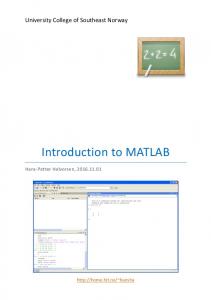
2.1 Temperature Control Problem and Physical Connections We are going to use a temperature process, where a temperature sensor is used, and the actuator of our experiment will be a lamp. The block diagram for a simple on-off controller is shown below.

Set point

ON-OFF Controller

Voltage

Process (Lamp) Temperature Sensor

Degree Celsius

Physically, we are going to connect the following, with the lamp placed within about a half centimeter of the sensor:

Controller implemented using some of the dSPACE features that we may find in the Simulink blocks. In this case, we will build a simple on-off controller, using the signum function, a couple of constants (one of them for the set point), and other useful elements.

DS1104 Analog Output (DACH1, pin P1A 31) DS1104 Analog Input (ADCH5, pin P1A 16)

Lamp

Temperature sensor

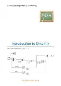
The circuits for the connection of the lamp and temperature sensor are shown below.

High current/voltage Darlington drivers 5 Volts

DS 2003

Analog Output

D1

Common DIODE

2.7k DS2

Q1 2N1070

PIN P1A 31

1 2

RESISTOR

LAMP

Q2 2N1070

5 Volts LM 35

7.2 k

3k

RESISTOR

RESISTOR

Temperature sensor

6 Volts 0.1 A E-5 base

Analog Input

PIN P1A 16

The objective of the temperature control system is to regulate the temperature at a fixed value in the face of ambient temperature disturbances (e.g. you blowing on the physical experiment).

2.2 Creating a New Experiment In ControlDesk, you create new experiments via the menu: File > New Experiment (note that we adopt the convention that italics are used for menu items and “>” is used to indicate a submenu). Using ControlDesk to interact with a real-time program running on the DS1104 requires the simultaneous use of a number of files.

These files are the generated executable program (*.ppc), variable description file used to relate to variables and parameters in the model (*.sdf), virtual instrument panels that you construct called layouts (*.lay), and possibly others depending on what actions you are performing. A ControlDesk “experiment” is the way you associate all these files to a single entity, thus the next time you need to run the same test you only need to load the experiment, which will automatically cause all the associated files to be loaded as well. When you create a new experiment via the above menu command, you get the figure below (well, a blank one; this one shows what was filled in) and you have to specify the experiment’s name, and the working root directory.

You do not have to fill the other fields, but it will be useful to have a history, and documentation concerning those fields so you may want to fill in some information in the “Author” and “Description Text” (as shown above). Note that while not essential you can create an “Experiment Graphic,” which is a graphic that can be used for illustration in the block diagram a window just above the “Ok” button in case you want to get a quick

overview of the experiment’s characteristics (see the simple control system block diagram of the temperature control system). The experiment will be saved with a “cdx” extension when you click “OK” and you will return to the ControlDesk.

2.3 Interfacing dSPACE Software to the Experiment Now that we have physical access to the signals via the above connections, we need to configure the software to interface to these signals. Suppose that you build an on-off controller in Simulink as shown below.

Digital to analog conversion block

Analog to digital conversion block

2.3.1 Digital to Analog and Analog to Digital Conversion Connections The construction of this block diagram will be discussed in more detail below. For now, focus on how we create the software interface between the controller and the plant (i.e., the interface that generates control inputs and read sensor values). The digital to analog conversion (DAC) blocks are provided in Simulink when the dSPACE software is available. Hence, we use a DAC block as shown above to generate the control input to the plant (i.e., the voltage signal to the lamp) and an ADC block to read the voltage from the temperature sensor that is proportional to the temperature. How do you define these DAC and ADC blocks? There are two ways to access the dSPACE blocks that can be used in Simulink. First, they are listed by typing simulink (note that here we use a convention of an italic

courier font when it is something that you type into the computer) in the Matlab command window (which, via ControlDesk you access by right-clicking on the Simulink icon in the upper left corner when the Platform tab is selected). The resulting window is shown below (note that if you double click on the last item on the bottom left you will see the dSPACE blocks for Simulink):

Another way to see the dSPACE blocks, and one that we will use here since it offers a few more features, is to type rti from the Matlab command window. If you do that the following window is shown:

If you double-click on each of these blocks, you are going to find the blocks necessary to build the simulation that you need. For example, if you double-click the icon called Simulink, you obtain the same elements that you would obtain if you typed simulink in your Matlab command window. Note that there are “Demos” that may be useful to you. Also, note that there is a “Help” button you may find useful. Next, we will discuss interface issues. The RTI1104 Board Library seen above is divided into some main sections. The I/O resources of the DS1104 are split between the two processors on the board, the Master PPC (Power PC) and the Slave DSP F240. By clicking on either one you will have access to blocks you can place in your model that provide I/O functionality associated with the respective processor. For this tutorial we will focus on the group of blocks contained in the Master PPC section. If you double-click on this you will get the following window:

As you see, this window has some of the most commonly used elements for the controller board, such as ADCs, DACs, Encoders, etc. If you double-click on any of these I/O blocks you will get it’s respective configuration dialog box, and one of the buttons you will see in this dialog box is “Help.” Clicking on this will launch the dSPACE HelpDesk exactly at the page referencing that particular block. Here, we clicked on dSPACE Help and downloaded the relevant information on the ADC and DAC that we need for the temperature control problem. You can also launch the dSPACE HelpDesk from the Start>Programs>dSPACE Tools>dSPACE HelpDesk, or if you are using ControlDesk you can launch it from the Help menu or simply by hitting the “F1” key.

2.3.2 Analog to Digital Conversion (ADC) and Signal Scaling First, we consider the acquisition of the sensor voltage signal. Note that we had connected the sensor to ADCCH5, pin P1A 16. To configure the software so that it can get this signal into the controller we click on “ADC” in the upper left corner (note the

label on the bottom of that button). In the window that comes up there is a Help button. If you click it, you will see:

•

DS1104ADC_Cx

Purpose: To read from a single channel of one of 4 parallel A/D converter channels. I/O mapping: For information on the I/O mapping, refer to ADC Unit . Unit page: Channel number Select a single channel within the range 5 ... 8. I/O characteristics: Scaling between the analog input voltage and the output of the block: Input Voltage Range Simulink Output –10 V ... +10 V

–1 ... +1

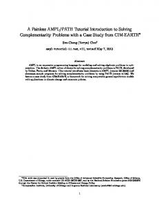
This tells you how to make the settings for getting the signal. Here, when you place an ADC block in a Simulink model (by drag and drop) and then double click it, all you need to select is the “Channel number.” In this case it is channel 5 due to the choice we had made for the physical connection of the temperature sensor (i.e., ADCH5, pin P1A 16). Next, it is important to understand the “scaling” that occurs in acquiring the signal. The physical input signal input range is –10V to +10V. dSPACE always scales this by a factor of 0.1 (multiplies by this number) to place the value on a range of –1V to +1V. This scaling typically needs to be corrected for due to the need to map the meaning of volts to temperature in degrees. This mapping depends on sensor characteristics, and is generally adjusted in Simulink blocks when the sensor signal is processed before it is used by the main part of the controller. This sensor signal preprocessing must also take into account calibration issues, such as knowing which voltage corresponds which temperature, and in general the mapping the voltage to temperature conversion needs to obey. For our temperature sensor we assume linear operation over the range of ambient temperatures, and 0.1 Volts corresponds to 10 deg. C, 0.15 Volts corresponds to 15 deg. C, etc. as shown below. Note that the slope of this line is 100.

Deg C 20 10

0.1

0.2

Volts

In summary, we need to take the ADC signal and multiply by 10 to remove the scale factor and then by 100 to represent the slope of the above line to convert Volts to Degrees, C. The resulting signal can then be used in the controller.

2.3.3 Digital to Analog Conversion (DAC) and Initialization / Termination

Next, we consider generating the voltage input to the lamp via DAC. Note that we had connected the lamp input to DACH1, pin P1A 31. To configure the software to generate this signal we click on “DAC” on the left side, third block down (note the label on the bottom of that button). In the window that comes up there is a Help button. If you click it, you will see:

•

DS1104DAC_Cx

Purpose: To write to one of the 8 parallel D/A converter channels. I/O mapping: For information on the I/O mapping, refer to DAC Unit . Unit page: Channel number Select a single channel within the range 1 ... 8.

Initialization page: Initialization value The initial output voltage at the start of the simulation. Value must remain in the output voltage range ±10 V. Termination page: Output on termination Either keep the current output voltage when the simulation terminates, or set the output to a specified value. Value must remain in the output voltage range ±10 V. I/O characteristics: Scaling between the analog output voltage and the input of the block: Simulink Input Output Voltage Range –1 ... +1

–10 V ... +10 V

The block provides its outputs in transparent mode, that is the channel is converted and output immediately. Initialization and termination During the model initialization phase, an initial output voltage value is written to each D/A channel. This is especially useful if a channel is used within a triggered or enabled subsystem that is not executed right from the start of the simulation. With the initialization value, the channel has a defined output during this simulation phase. When the simulation terminates, the channel holds the last output value by default. You can specify a user-defined output value on termination in the Termination page, and use these settings to drive your external hardware into a safe final condition.

Here, note that if you place a DAC block in your Simulink model and double click it there are several settings that need to be made (note the tabs near the top of the window). First, on the “Unit” tab you need to select the channel number; here it is channel 1 (DACH1, pin P1A 31). Next, under the “Initialization” (“Termination”) tab you pick the initial (final) voltage value. Depending on which experiment you hook up, the choice of these values can dictate smooth and safe operation of the experiment (e.g., so that you do not hurt the experimental equipment). For instance, if the initial value for some mechanical system were 10V, then this may correspond to spinning a motor at its maximum rotational speed. Note that in general these values should be viewed as the ones that are input to the plant immediately before and after the actual control system operates. Hence, for example, if you initialize the output to be zero there may be a sharp change at the first sampling instant when the controller may put out a different value (analogous comments hold for termination). Note that such a sharp change is something that you may have to pay attention to in an actual implementation since it can have effects on the transient response (e.g., for some experiments you may want to make sure

that the initial transients due to such effects have died out before you test the response of the system to a step set point change). Here, since the dynamics of the temperature process are so slow, we ignore the effects of such possible transients and simply set the initialization and termination values to zero. The precise meaning of Initialization and Termination in a real-time program running on the DS1104, and when are they executed, are discussed in the following section, which also explains what “real-time” is and what the basic structure of a real-time program looks like. As we can notice, we added before this block a scale gain of 2/10, due to the dSPACE scaling factor that we saw in the input, but now it should be reversed when it goes to the exterior (1/10), and since the Darlington device switches when the input voltage is greater than 2 volts, we have to add this value of 2 in the gain.

2.3.4 Real-time and the Structure of a Real-Time Program What is real-time? You have a physical system or object you wish to control with a program, much like the experiment detailed in this tutorial. Because this system or object has certain dynamics associated with it, you have to control it based on those dynamics. Therefore we say that the physical system will have a time constant, from which you will derive a step size or sample time for your control program. The challenge is to not only use that sample time in the numerical calculations that make up your control algorithm, but also to execute that algorithm within that sample time. You have to start each “step” of your program exactly one sample time or step size apart, and thus have to finish the computation of each step within the sample time, i.e. before the next step starts. This is real-time. Please see the diagram below.

Program executing Idle time

0

T

2T

3T

If the sample time of our program is T, you can see that the program is executed at distinct points in time that are one sample time apart. You will also note that each step of the program finishes executing before the next step is due to start; thus this program is running in real-time. If however the computational demands of the program cause the processor to take more time than the sample time then we have an Overrun condition, and our program cannot run in real-time. Later on the overrun condition is discussed further. The overall structure of a real-time program can be simplified for explanation purposes into three main sections: Initialization, the real-time task or tasks, and the background. The initialization section is code that is executed only once at the start of execution, upon download of the program. In this section you will have functions that, for initialization of the system, are only needed to run once. The next part of the program is the real-time part, the task, represented by the gray sections in the diagram above. This is what is executed periodically based on the sample time. This part is the heart of the control program; for this, you read inputs (e.g., from an ADC), compute your control signals, and write outputs (e.g., with a DAC). Note that depending on what your control application is you may have multiple tasks in your model. Finally, the last section is the background; this is code executed in the “idle” time between the end of computation of a step and the start of the next step.

2.4 Controller Development in Simulink In this section we will discuss how to use Simulink for controller design and how to compile the Simulink model into code that will run on the dSPACE board for real-time implementation of the controller.

2.4.1 Simulink for Controller Design Now that we have the signals that we need to sense and actuate we can consider the development of the Simulink model of the controller shown below:

Controller

As you can see in this example, we used a constant to fix the set point (of course we could have set it to be a square wave or some other time varying function). We chose 20 deg. C since this corresponds to 68 deg. F and the typical temperatures in our lab range from 18 deg. C (64.4 deg. F) to 22 deg. C (71.6 deg. F) so this value is in the middle. Later we will change this value to see how the control system reacts. The sign function fixes the output depending on the sign of the error (since we do not want a negative output in this case, we used the min-max function to choose a positive value, when we compare with 0). Then the controller operates by computing the error between the set point and sensed temperature. If the error is positive, then the sensed temperature is below the set point so the controller turns the lamp on. If the error is negative, then the sensed temperature is above the actual one so the lamp is turned off and the ambient temperature must lower the temperature in the region around the sensor.

2.4.2 Building the Simulink Model

Once we define the model, we have to change some parameters in the simulation. To do this, in the Simulink model, use Simulation > Simulation Parameters… and you will see the following window.

The most important steps to take into account are described in the following figures. First, in the Solver options (see tab) set the “Start time” to 0 (needed for real-time applications). The “Stop time” can be set according to how you want the experiment to run. If you set it as “inf” it will go forever, but if you set it to 20 it will run the experiment for 20 sec. Next, set the “Type” to a Fixed-step option, and pick a solver such as “Euler” or perhaps “ode5.” Note that the more complex a solver you choose the more computationally intensive your program will be and thus will require more time to execute. Next, pick the sampling time for the experiment. This is the sampling rate, which is typically denoted by “T” in digital control books, and it sets the sampling rate for the sensed signals and control updates. If you have a controller that demands too many computations within the sampling period such that they cannot be completed in time, then you will encounter an overrun condition and you will get an error attesting to this upon download of the program to the DS1104, and you will have to raise the

sampling rate. For our temperature control problem we choose T=0.0001 sec. so we get the following:

After you change this, go to the Advanced option tab, and as it is suggested at the beginning of the Matlab program that you should have the Block reduction option Off so do that to obtain the next figure:

Once you followed these steps, you are ready to build the model. You have two options: the “short-cut” command CTRL-B (from within the Simulink model) or go to Tools > Real-Time Workshop > Build Model. The build process will then commence, during which you will be asked what to do if there is an “overrun” via the following dialog box:

As explained before, an overrun situation occurs if a task is requested to start but has not finished its previous execution yet. By default the option will be set to “stop simulation (set simState to STOP)”, you want to keep this default. We want to be able to detect if the program is running in real-time or not and if we choose to ignore overruns we may not be running in real-time and never realize it.

After you click “OK” in the dialog box above the build process will continue. C code is generated for the model and then this code is compiled and linked by the Power PC compiler (since the DS1104 uses a Power PC processor) to produce a single executable object file with a .ppc extension. This executable is then downloaded to the DS1104 and the program starts running (i.e., executing the controller). If there are any errors during the build process or you run into an overrun condition this will be printed in the Matlab command window, otherwise if all goes well you will see the message “Build Succeeded” in Matlab. You can stop the program on the DS1104 by clicking in the Stop button that is located in the ControlDesk, on the toolbar across the top (its icon is a small red box). Note that stopping the program this way means stopping the whole program, thus the real-time task and the background routine, and that this way will not execute or enable functions associated with the termination state, such as the termination values for the DAC channel. To enable the termination condition or state you have to stop only the real-time task, and changing a certain variable in the program does this.

2.5 Graphical User Interface to the Experiment In this section we discuss how to create a graphical user interface (GUI) for the user so that they can view on the screen various aspects of the operation of the running control system (analogous to hooking up an oscilloscope in some cases), make changes while the control system is operating (e.g., changing controller gains or set points), and viewing and saving data for plotting and reports. First, we must have a “layout” file for the dSPACE experiment. To do this, use File > New > Layout. Next, you use View > Controlbars > Instrument Selector. This shows the items that can be used to make a GUI interface. First note that there are two instrument types: Virtual instruments and Data acquisition instruments. These instruments are showed below. time.

You can ignore the Custom instruments group at this

When you generate a layout that you associate with the experiment, you can link any of the variables that you created in your Simulink model to it. When you build your Simulink model, two of the files generated are the Variable Description File (*.trc) and the System Description File (*.sdf). If ControlDesk is open when your model is built and downloaded to the DS1104, you will see that the associated .sdf file will automatically be loaded into the variable browser in the Tool Window. If ControlDesk is not open when the model is downloaded you will need to load the file by using File > Open Variable File, then selecting the appropriate .sdf file. Once the variable file is loaded you can link variables in your model to graphical instruments on layouts. In order to do so, you need to locate the variables in the variable browser and then drag and drop them onto the respective instruments on the layout. The variable browser (that is shown in the next figure) has two areas: the variable tree (the one which is at the bottom left of your screen), and the variable list that is at the bottom right. The variables that you are going to associate with each of the layout instruments are pulled from the variable list. When you create a graphical instrument on a layout and it is not yet associated with a variable it will have a red border. Once a variable is linked to that instrument on your layout the red border will turn black. If you right-click over any created instrument on a layout you will obtain a menu, on which you will see “Highlight variables”. If you select this, every time you click on an instrument that is associated with a variable you will see that particular variable highlighted in the variable browser.

Variable tree

Variable list

Using all of these elements, we built a layout for our temperature control problem that is shown below. To add each of these instruments we clicked on the instrument group containing the instrument, then we clicked on the icon of the instrument, and finally in the instrument panel (what we called the layout), and using the mouse we drew some rectangular instruments. In this example, we used a bar to display the voltage input, a display to show the output value, a numerical input to adjust the set point, and a plotter to show a variety of values. The plotter, as you can see in the next figure, has many variables associated with it (i.e. in the bottom left of the figure, you will see different colors, and that means that you are plotting more than one variable). For this case, the error, set point, output, and the scaled input are the variables associated with the plotter. If you click any of the colored boxes you will see the associated variable name on the Yaxis. Note that if you drag and drop variables onto the Y-axis of the plotter it will put all those signals on the same Y-axis. If you drag and drop variables onto the X-axis or onto the main body of the plotter it will create a new Y-axis for each signal dropped this way, which is useful if you want to view multiple signals on the same plotter but the signals have very different ranges.

We can change some properties concerning each of the elements of the layout. For instance, we can limit the range of the numerical input to avoid that the user changes the set point drastically. For that we double click in this element, and we obtain the following:

Here, we put the increment of 0.1 degree, and the set point is going to be between 18 and 26. The user cannot put a value greater than these limits, because with the current environment it doesn’t make sense to have more than these values. After you create the layout(s) (yes, you can have more than one for an experiment) you will have to add this layout and the variables that you associated to it, to the experiment (i.e., when you load this experiment, all the files will be reloaded with it, and so the links created in the process described above). For that, go to File > Add All Opened Files, and then save the experiment using the command File > Save Experiment. If you do have multiple layouts in your experiment you can select View>Workbook, this will create tabs for each layout enabling you to switch easily form one to another. Once we built all the components in the Edit Mode, we switch to the Animation Mode (shortcut F5 or click in the icon as we show below). This mode allows you to control the variables of an application (change parameter values or data connections), observe the signals with data acquisition instruments and capture data and save the results to disk for later analysis and plotting in, for example, Matlab for lab reports. The data is

now being transferred from/to the simulation platform, and you can work now with other external devices. While in this mode, you might change the parameters of the variables at least the ones that you allowed to be changed, such as the output voltage and so on. In addition, you can also capture data or observe some signals with the data acquisition instruments (e.g., the plotter).

Edit Mode

Animation Mode Test Mode

2.6. Capturing Data1 There are two main methods of capturing data to a file or multiple files. If you assign a variable to a plotter instrument you not only can see the signal you can also cause the data to be saved to a file. However, if you do not need to see the signal but simply capture or acquire it, then you can do that as well. Both these methods use the exact same mechanisms in ControlDesk, one just also displays the signal.

The

mechanism used to control and parameterize data capture is the CaptureSettings window.

2.6.1 Data Capture With the Plotter You are familiar with viewing a variable on a plotter by a drag and drop action. To set ControlDesk to store that data to a file you must launch or access the CaptureSettings window. There are three different ways to do this: a. Click the button shown below that appears in the variable browser 1

CDExpGuide pags. 298-310

b. Right-click over the plotter and select “Edit Capture Settings”; in most cases the ensuing CaptureSettings window will appear on the very right edge of Controldesk as shown below and you will have to expand it

Expand

c. Select the CaptureSettings instrument from the Data Acquisition group and place it on a layout.

Once you have accessed the CaptureSettings window it will appear as follows:

You can click on the “Settings” button and you will get the CaptureSettings Control Properties box. Please click on the Acquisition tab, you will then see the following:

Explanation of the options on this page is as follows: Simple: Select this radio button to perform a simple data capture. This mode captures only a period of the signals into the buffer. Even if you select Auto Repeat, two consecutive captures are independent of one another. For example, there may be a delay between them. Autosave: Select this radio button to activate the capture to be stored to the MAT/CSV file (*.mat as a MAT file that can be used in Matlab for some manipulations, or *.csv to use in some spreadsheet packages as Excel) specified in the edit field. Click the Browse button to select the MAT/CSV file or enter a new name. The captured data is written to the specified file. If you perform several data captures, the older data is overwritten by the new data. Autoname: Select this radio button to enable automatic file naming. Click the Browse button to select a MAT/CSV file or enter a new name. The filename is extended by an index that automatically increases for each data capture. Each capture is stored in its own file. Continuous: Select this radio button to activate continuous capturing. The continuous mode captures data without gaps from the simulation platform using a cyclic buffer. You have to stop the capture explicitly. Stream To Disk: Select this radio button to activate data capture streaming to the IDF file specified in the edit field. As long as Stream To Disk is active an additional icon (yellow disc) is displayed. Click the Browse button to specify a different file and path for the continuous capture storage IDF file. Show Graphic Output: Graphics output is enabled by default. However, displaying the data reduces the rate of data transmission to disk. Unmark this checkbox to save

computing power. Show Graphic Output is only available for Autoname, Autosave and Stream To Disk. Assuming you have launched the CaptureSettings window, let us examine the parameters or options you have to set. Length: This specifies the actual length in seconds of the data capture, the x-axis,, thus if you selected “Autosave” as your acquisition method, data in the stored file will correspond to that length. Downsampling: This refers to how often you want to capture a point of data, i.e. if downsampling is 1, it means capture the value of that variable every single step or sample of the program; if we set it to 3 it means capture a data point only every three steps. If you are working with slow dynamics or transients you may want to increase the downsampling. If you are using “Continuous” as your acquisition mode you may need to use a higher downsampling value to avoid problems with hardware coping with capture rates and memory limitations. Auto repeat: If you are using “Simple,” “Autosave,” or “Autoname” modes of acquisition selecting this option will enable consecutive captures to start automatically. Trigger signal: If you want to trigger your data capture to start based on another variable in your model you can drag and drop that variable onto the gray field with the caption “ > “, you can then set with the other fields which edge you wish to trigger on: rising or falling, what value level to set the trigger condition on, and if you want to pre- or post-trigger by providing a negative or positive delay value. This is very much like features on a regular oscilloscope.

2.6.2 Data Capture Without the Plotter

As mentioned earlier, you can capture data to a file without using a plotter. You can select the variables to capture this way by two methods: a. Locate the variable in the variable browser you wish to capture, then drag and drop it onto the #1 button on the right side of the variable browser b. The same as above except drag and drop it onto the CaptureVariables icon on the CaptureSettings window), illustrated next:

Drop variable on this icon

Configure the desired settings as discussed in the previous section. To verify the connected and used variables you have to follow the next steps: •

In the Capture Settings Instrument, click “Settings” to display CaptureSettings Control Properties dialog.

•

In the CaptureSettings Control Properties dialog, choose the CaptureVariables page

The variables connected to the Data Acquisition Instruments can be identified by the icon displayed in the first column (Connected). The connected variables will always be used for data capture. If you have only selected a capture variable for data capture, no icon is displayed in the first column. To use the variables, mark the checkbox in the second column (Measurement). The figure below shows the CaptureVariables tab that we use to choose the variables that we are going to store.

Data capturing starts immediately after the animation starts, if the checkbox Auto start with animation on the Capture property page in the CaptureSettings Control Properties dialog is marked. Otherwise, use the Start/Stop button to start and stop the capture manually.

3. Exercise: Implement a Temperature Control System in dSPACE Here, we ask you to conduct a simple exercise to help you get acquainted with dSPACE. The general idea is to sense the temperature that is measured using the LM35CAZ, and try to turn on/off two different lamps using 1 analog output and 1 digital I/O. For that, we are going to build the model that is shown in the next figure.

The hardware that you have to build is the following:

The data sheets for all the components that we are going to use to build the experiment are on the web.

If you study the model that you are going to build you can see a loop very similar to the one that we show in the tutorial, but instead of having an analog output, we are going to use a digital output. For that, we have to convert the output that comes from the MinMax block, since this output is a double value. We then use the data type conversion block (which you will find useful in other applications). We put two examples in this exercise, since in the lower loop we are comparing the value of the error with some value. Since the output in this case is Boolean, we have to convert it again to a double, since in that case the analog output uses double values. You have to develop the same diagram as above, and go step by step to compile it correctly, such that it runs in dSPACE. The sampling time could be select as 10 ms, and the solver could be ode5. Now, once you build the model, you have to create an experiment in dSPACE. Follow the steps before, and then you have to: 1. Put a plotter to show the input value, and the signal that is coming from the sensor. 2. Take two numerical inputs, such that one of them handles the set point, and the other one handles the constant that is in the lower loop, i.e. the one that you are comparing with the error. The first numerical input must have a range between 19 and 25, and the increment must not be greater than 0.1 (pick what ever you want). The second numerical input must have increments of 0.05, and you pick the range according on what you think is the best performance of your controller. 3. Take a display, and show in this element the temperature value sensed by the sensor, after the appropriate scaling. 4. If you want to put anything extra in, do it, and show your work to the TA.

4. Notes and Tips for Signal Conditioning2 The following notes and tips may help you to achieve optimum results using ADCs and DACs.

•

Crosstalk

Crosstalk occurs if a signal with steep edges runs close to a high-impedance analog signal. The main reason for crosstalk is inductive coupling. Crosstalk can be reduced or avoided by the following measures: ÿ Twist each signal with its return line (ground) and separate digital and analog signals. ÿ Never use a twisted pair cable for different signals. ÿ Route wires of ADC inputs separately from wires of DAC outputs. ÿ For ADC: drive the inputs with a low-impedance output (although the input resistance of the converters is very high).

•

Grounding

All return lines are connected to a system ground. To avoid ground loops, use separate return lines for all connected sensors/actuators. Sensor/Actuator grounds should be isolated from each other. Ideally each signal should be twisted with its return line (ground) so that their electromagnetic fields cancel. The ground return lines must be connected on both cable ends. If not enough ground pins are available at the connector several return lines can be attached to a common ground pin. However, this common ground lead should be kept as short as possible to reduce ground line inductance. ¸ The following notes and tips may help you to achieve optimum results using the BIT I/Os.

2

Installation and Configuration Guide, Connecting External Devices to the dSPACE System.

•

Unconnected I/O pins are set to a defined logical high-level built-in 10 kW pull-up resistors, which are connected to +5V. To force a TTL input to a defined logical lowlevel, an external pull-down resistor of about 1 kW can be connected to GND.

¸ The following notes and tips may help you to achieve optimum results using the INCREMENTAL ENCODER INTERFACE.

•

To allow proper operation, do not connect the outputs of your encoder to an ACcoupling network. The input signals must be DC signals.

•

The connectors for the incremental encoders offer two VCC pins. You should connect both pins so that both pins share the current evenly and the voltage drop in the lead wires is kept as small as possible.

•

The total load of ALL connector pins that provides access to the PC power supply must not exceed 500 mA.

•

If you use an external supply voltage, you have: ÿ To guarantee that no input voltages are fed to the DS1104 while is switched off ÿ To connect the encoder’s ground line to a ground pin of the board (page 102).