A Tutorial Introduction to Supervisory Hybrid Systems - University of

A Tutorial Introduction to Supervisory Hybrid Systems Technical Report of the ISIS Group at the University of Notre Dame ISIS-98-004 October, 1998

M.D. Lemmon, K.X. He, and I. Markovsky Department of Electrical Engineering University of Notre Dame Notre Dame, IN 46556

Interdisciplinary Studies of Intelligent Systems

1

A Tutorial Introduction to Supervisory Hybrid Systems Michael D. Lemmon , Kevin X. He, and Ivan Markovsky Department of Electrical Engineering University of Notre Dame October, 1998

Abstract Supervisory hybrid systems are systems generating a mixture of continuous-valued and discrete-valued signals. These systems provide convenient models for a wide range of complex engineering applications ranging from small real-time embedded systems to large-scale traffic control and manufacturing facilities. In recent years there has been considerable interest in using hybrid systems theory to develop a systematic framework for the analysis and design of complex engineering systems. This paper provides an introduction to some of the concepts and trends in hybrid dynamical systems theory.

1 Introduction Supervisory hybrid systems are systems generating a mixture of continuous valued and discrete valued signals. This systems paradigm is particularly useful in modeling applications where high level decision making is used to supervise process behavior. This occurs, for instance, whenever a network of computers is used to control the physical plant in a decentralized manner; as is found in chemical process control or flexible manufacturing facilities. Hybrid system methodologies are also applicable to switched systems where the system switches between various setpoints or operational modes in order to extend its effective operating range. Such applications are found in aerospace and power systems. Hybrid systems, therefore, embrace a wide range of applications [32] [71] [75] [76] [77] [78] [79] ranging from embedded real-time systems to large-scale manufacturing facilties, from aerospace control to traffic control. Over the past 5 years there has been considerable activity in the area of hybrid systems theory and this article provides an introduction to some of the basic concepts and trends in this emergent field. The term hybrid refers to a mixing of two fundamentally different types of objects or methods. Hybrid neural networks arise when we combine artificial neural networks with fuzzy logic or with statistical methods. A system modeled by the interconnection of lumped and distributed parameter systems may be referred to as a hybrid system. Sampled data control systems are hybrid in that they combine discrete-time and continuoustime systems. This paper deals with supervisory hybrid systems. Owing to the diverse useage of the term hybrid, we need to be precise in delineating the hybrid nature of these supervisory systems.  We gratefully acknowledge the partial financial support of the Army Research Office (DAAH04-96-10285 and DAAG5-98-1-0199) and the National Science Foundation (NSF-ECS95-31485)

2

System science provides a formal mathematical approach to the study of dynamical systems. The system scientist treats the system as an abstract mathematical mapping between various sets of signals. The signals are, themselves, functions between a set of time indices, I, and a set of measurments M. Signals, therefore, are functions of the form x : I ! M which map a time t 2 I onto a measurement x(t ) in the set M. Hybrid systems arise when they generate signals whose index or measurement sets can be treated as the Cartesian product of a discrete and continuous set. The obvious example, in this case, is the class of sampled data systems in which the index set I is the Cartesian product of the integers (discrete-time) and real numbers (continuous-time). Supervisory hybrid systems, on the other hand, arise when the measurement set M is the Cartesian product of a discrete set (usually taken to be a finite set of symbols or integers) and a continuous set (usually taken to be some subset of Euclidean n-space). The discrete-valued signals are sometimes referred to as discrete-event signals. The hybrid nature of supervisory hybrid systems, therefore, is a consequence of the fact that these systems generate a mixture of continuous-valued and discrete valued signals. This paper is concerned with the study of supervisory hybrid systems. A common example of such systems is found whenever a computer is used to supervise the behavior of a continuous-valued process. The continuous process may be a closed loop control system whose mathematical representation takes the form of an ordinary differential equation. The computer program may be seen as supervising this control loop by selecting various reference inputs. This program’s current state evolves over a discrete set and the dynamics of the associated discrete-event process are formally modeled using language theoretic or graph theoretic constructions. We therefore see that this computer supervised system is a hybrid system since it mixes continuous-valued (the control loop’s state) and discrete-event (the program state) variables. Over the past five years there has been considerable interest in supervisory hybrid systems [63] [64] [65] [66] [67] [68] [69]. One of the primary motivations for this interest rests with the fact that rapid advances in computer and networking technology have greatly accelerated the deployment of large scale supervisory systems. Examples of such large scale systems include the air traffic control grid, communication networks, and the power distribution grid. Traffic control is concerned with the supervision (a discrete process) of vehicles (continuous processes). Congestion control in communication networks is similar in that we’re interested in supervising the flow of data packets so that some continuous-valued measure of service quality is optimized. Power distribution involves discrete switching to ensure the stable and continuous delivery of electrical power across the grid. The safe operation of such systems is of paramount interest to the nation as these systems constitute major components of the national infrastructure. Current methods for the design and analysis of such systems rely heavily on simulation testing which is a costly and time consuming method of analysis providing no provable guarantees of safe system operation. The hope is that hybrid systems theory will provide a systematic framework for system engineers that will greatly reduce the cost of large scale system development with concurrent increases in system reliability. The remainder of this paper is organized as follows. Section 2 provides a concrete example of a hybrid system which will be used throughout the paper as a pedagogical tool illustrating various concepts in hybrid systems theory. Section 3 discusses modeling frameworks for hybrid systems with specific attention being paid to the hybrid automaton in section 4. Not only may the system have a hybrid character, but the specifications on desired system behaviors may also be hybrid. Section 5 discusses specification logics for hybrid systems that express system requirements on both the discrete and continuous states of the system. Section 6 surveys current methods and concepts used to verify or validate desired system behaviors and then concludes with a survey of current methods for hybrid control system synthesis. Final remarks will be found in section 7.

3

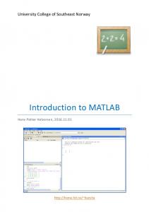
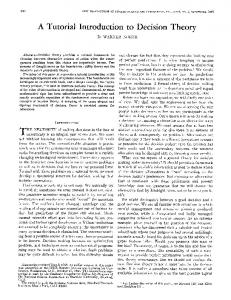
2 Hybrid System Example A concrete example of a supervisory hybrid system will be found in figure 1. This figure shows a free floating robotic vehicle with two articulated arms. The system is required to obtain components from a parts bin and move these components to a work area where an assembly operation is to be performed. The tasks of fetching the workpiece, transporting it to the work area and then returning to the parts bin to fetch another workpiece are performed repeatedly. As illustrated in figure 1, however, it is assumed that the parts bin is shared by both robotic arms. The introduction of a shared resource (i.e. the parts bin) generates a mutual exclusion requirement on the system. Not only must the robotic arms complete their repetitively performed tasks, they must also be sure to execute the tasks in a way that ensure both arms don’t enter the parts bin at the same time. In other words, the robotic system needs to treat the parts bin as a critical section which both arms access in a mutually exclusive manner.

y

D1 A1 B

θB

θ’1

θ1

PB

θ2 θ2’ D2 A2 Figure 1: Free Floating Robotic System A candidate solution to the mutual exclusion problem can be readily developed [58] [59] [62]. Let’s assume that each arm is controlled by a computer process (an instantiation of the arm control program). We therefore have two concurrently running computer processes that need to coordinate their actions if they are to ensure the physical system (i.e. the robotic arms) enters the parts bin in a mutually exclusive manner. Assuming that a multi-tasking operating system (O/S) controls the execution of both computer processes, we can then use O/S control structures such as semaphores or mutexes [60] to ensure that both processes execute, in a mutually exclusive manner, that section of their code requesting access to the parts bin. In other words, by requiring that the virtual (i.e. computer) processes respect the mutual exclusion requirement, we hopefully expect the robotic arms (i.e. the physical system) to respect that requirement as well. The pseudo-code for one of the computer processes is shown below

4

x

ENTRY: if(x==1) goto ENTRY x=1; CRIT1: if(arm_not_in_partsbin) command_arm(1); EXIT: x=0; ERR: if(arm_locked) STOP; REM: if(arm_not_in_workarea) command_arm(-1); goto ENTRY;

This code segment has four distinct segments. There is an entry section (ENTRY) which tests the lock variable x to see if the other arm is moving towards the parts bin. In practice, the lock variable could be implemented as a O/S semaphore. If the lock variable x is 1, then the program sets the lock variable to alert the other process that it is heading to the parts bin. This process then enters its critical section (CRIT1) which represents that code which must be executed mutually exclusively. In other words, both computer processes cannot be executing their critical sections at the same time. While in the critical section, the program checks to see if the arm is in the parts bin (the function call arm_not_in_partsbin) and outputs the command signal to the arm’s motor (the function call command_arm(1)). Upon leaving the parts bin, the process releases the lock variable and then enters its remainder (REM) section from which it commands the arm to move back to the work area. This remainder section checks to see if the arm is in the work area (the function call arm_not_in_workarea) and ouptuts the command signal to the arm (the function call command_arm(-1)) which moves the arm towards the work area. We’ve also included an error state (ERR) in the program that aborts the program’s execution if the arm hits its mechanical limits (i.e. arm_locked evaluates to true). From this pseudo-code, we see that the state of the program can be characterized by 3 different state variables; the lock variable, the program counter for the first process and the program counter for the second process. Since these variables take values in a discrete set, the supervisory logic embodied in this program is a discrete event system. Whether or not ensuring mutually exclusive execution of the process’ critical sections is sufficient to guarantee the safe operation of the physical system is not immediately apparent. From our earlier discussion, we saw that the computer process controlling each arm occupies a number of distinct states. Are these discrete states sufficient to represent the behavior of the physical process? For this particular system, the answer is negative because there is a subtle coupling between the arm and body dynamics. The equations of motion for the arms can be expressed by the following ordinary differential equations θ¨ 1 θ¨ 2

= =

θ˙ 1 + k(θ1 + θb θ˙ 2 + k(θ2 + θb

r1 ) r2 )

(1)

where θ1 and θ2 are the angular positions of arm 1 and arm 2 with respect to the robot’s body axis (see figure 1). For this example, we see that the control law is a proportional feedback law with gain k and with reference inputs r1 and r2 . These reference inputs represent commands that direct the arm to move to the parts bin or work area. Due to the Hamiltonian nature of the system, the movement of the arms will induce a body rotation so that the system’s total angular momentum is conserved. We therefore know that the body angle θb with respect to an inertial frame must satisfy Jb θ˙ b + Jaθ˙ 1 + Ja θ˙ 2 = 0 where Jb and Ja are the moments of inertia for the body and arms, respectively.

5

(2)

Note that the state of the continuous-valued subsystem is not entirely reflected in the discrete-event state of the computer process. Transition between discrete states is triggered on the entry into or exit from the parts bin and this knowledge is determined by explicitly examining the arm’s position with respect to the position of the parts bin. by measuring θ1 + θb . We assume that the computer process can only measure θ¯ 1 = θ1 + θb , the angle between the arm and the parts bin (or work area). Under our assumptions, it is assumed that the body angle cannot be obtained independently from θ¯ 1 . The fact that the arm angle, θ1 , (relative to the body) and body angle, θb are not directly observable suggests that it may be possible for this system to fail in ways that cannot be predicted by an examination of the controlling computer processes. From equation 2, we see that arm motions will induce a body rotation since the system conserves total system angular momentum. It may, therefore, be possible for the system’s body to work itself into a position from which one of the arms cannot reach the parts bin. If this were to occur, then the system would deadlock (i.e. the program would be get stuck in one of its discrete states). In other cases, system dynamics imply a subtle coupling between both arms which might make it possible for an arm to enter the parts bin when the controlling computer process is not in its critical section. As a result, it is possible to violate the mutual exclusion constraint without the computer process actually detecting this violation. The conclusion to be drawn from the preceding discussion is that even relatively simple systems such as that shown in figure 1, may need to be studied using a formal framework in which both discrete and continuous system dynamics are examined simultaneously. The goal of hybrid system science is to provide such a formal framework and the following sections discuss what progress has been made to date in this direction.

3 Hybrid System Modeling Hybrid systems have been studied extensively by computer scientists and system scientists. Computer scientists have been interested in the behavior of real-time and multi-processor programs. The system models developed for such systems are usually based on extensions of traditional finite state machine or Petri net formalisms. System scientists, on the other hand, have tended to employ equational models in which system trajectories are represented as functions solving some set of equations. Each approach has its strengths and weaknesses. What has become apparent in recent years is that a successful modeling paradigm for hybrid systems must integrate ideas and methodologies from both disciplines in a complementary way. Early system theoretic models for hybrid systems tended to focus on switched systems [74]. These are systems that can be implicitly modeled by the following set of equations, x˙

=

i(t )

=

f (x(t ); i(t )) q(x(t ); i(t ))

(3) (4)

where x : ℜ ! ℜn is the continuous valued state trajectory and i : ℜ ! Ω is a discrete valued state trajectory taking values in the discrete set Ω. x(t ) and i(t ) denote the values that the continuous and discrete trajectories take at time t, respectively. The function f : ℜn  Ω ! ℜn represents a set of continuous dynamical systems (vector fields). The dynamical system used at time t is represented by the discrete state i(t ) at time t. The dynamics of the discrete state are embodied in equation 4. In this equation, i(t ) = limτ"t i(τ) represents the righthand limit of the function i(t ) at t. Equation 4 means that the discrete state transtions at time t from state i(t ) to i(t ) and that this transition is conditioned on the current value of the continuous state, x(t ). The set of discrete sets we might transition to is characterized by the discrete transition function, q : ℜn  Ω ! Ω. It is convenient in switched systems to define a switching set between the ith and jth subsystems by the 6

following equation,

Ωi j = fx 2 ℜn : j = q(x; i)g

(5)

This set is the set of all continuous states which enable a transition from discrete state i to discrete state j. We usually assume Ωi j is a ”nice” set in the sense that its boundary is an n 1-dimensional manifold (a hypersurface). We therefore see that the switching action may be initiated whenever the system’s continuous state evolves across that boundary. A natural question to be asked about such equational representations is whether or not they are well-posed. In other words, are there any continuous or discrete trajectories that satisfy these equations? Conditions for the existence of absolutely continuous trajectories generally require that a set-valued mapping associated with these system equations be upper semicontinuous and convex [7]. These are very general conditions and are satisfied by most of the systems of interest. The existence conditions [7], however, do not preclude the existence of hybrid system continuous state trajectories which are not absolutely continuous. Switching systems of the form shown in equations 3 and 4 are well known to exhibit chattering solutions in which the system switches infintely fast between two different types of vector fields. The existence and exploitation of this relaxed behavior is, in fact, a basic principle behind another important class of hybrid systems known as variable structure systems [8]. It is interesting to note that computer scientists also have an interesting term for this chattering behavior. Systems capable of exhibiting such chattering solutions are sometimes referred to as Zeno systems. The name refers to the classical Zeno’s paradox in which the concept of a limit is first informally introduced. In supervisory hybrid systems, we want all of our systems to be non-Zeno. While we can usually ensure the existence of solutions to such equations, there is no guarantee that these solutions will be unique. The switching systems represented in equations 3 and 4 can also be treated as differential inclusions for which it is well known that nondeterministic solutions exist. In other words, if we know the system state at time t, the future behavior of the system may take any one of a number of different paths. This nondeterminism is, in fact, a fundamental property of hybrid systems and it represents one important way in which hybrid systems theory differs from traditional linear systems theory. The switching system introduced in equation 3 and 4 provides a convenient model for many physical systems, but it does not capture the full range of possible hybrid behaviors. The preceding model assumed solutions in which the continuous state trajectories were continuous across the switching boundary. There are, however, many systems in which the continuous state makes discontinuous jumps on the switching boundary [6] [5]. One example of such a system is the bouncing ball where, due to an elastic collision, the ball’s velocity vector makes an instantaneous sign change upon hitting the floor. A variety of hybrid system models have been developed to allow the representation of such discontinuous or autonomous jumping. A good reference to some of these models will be found in [4]. The preceding references to the hybrid system’s modeling literature refer exclusively to the efforts of traditional system scientists. These scientists were trying to develop an equational framework capturing a sufficiently rich array of possible hybrid behaviors (chattering, switching, and autonomous jumping). A key challenge to be faced by any hybrid systems paradigm, however, involves developing a framework which not only treats continuous-state jumping, but also captures the switching nature of the discrete-event process. Equational representations familiar to most system scientists, unfortunately, do not provide a convenient way of capturing discrete event behaviors. What is really needed for hybrid systems theory to advance is a modeling paradigm providing greater insight into the discrete event dynamics of the hybrid system. An early hybrid system model dealing explicitly with discrete and continuous dynamics will be found in

7

[9]. In this case, the hybrid system was viewed as logical discrete event supervisor connected to a continuous subsystem. The discrete and continous systems were interconnected through an interface that transformed continuous-valued measurements into discrete event signals and vice versa. This work suggested a logical discrete-event system (DES) approach to hybrid controller synthesis which was reminiscent of traditional approaches to sampled data control. The approach advocated the extraction of an equivalent discrete-event model of the continuous subsystem which could then be supervised using extensions of the Ramadge-Wonham supervisory control theory [61]. While providing a very general framework for hybrid systems, the model in [9] [11] [10] was of limited utility due to the restrictive nature of the control. A framework with significant potential for practical useage was developed by the computer science community [1] [2]. Computer scientists have long used formal graph theoretic models for concurrent computer processes. Finite state machines and Petri nets represent two well known examples of such models and while powerful computational tools were developed for the manipulation of such formal models, it was apparent that in dealing with multiprocessors and real-time applications, that the continuous nature of time would require some extension of these traditional computer science methodologies. This realization led to an attempt to extend traditional and highly successful model checking [28] for finite state machines to real-time systems. The result was a timed [2] and hybrid automaton [1] . These automata were generalizations of traditional finite state machines in which event transitions were conditioned on the truth value of logical propositions defined over a set of continuous-valued dyanmical processes. The work was very influential in that it led to the development of verification tool [3] [22] [23] [27] for real time and hybrid systems and has served as the starting point for much of the recent research in hybrid systems. The hybrid automaton is closely related to the differential automaton which was introduced in [13] [70]. Another related version of the hybrid automaton will be found in [14]. Extensions of the approach using Petri nets (rather than finite state machines) will be found in [15] [46] [16] [17] [18] [19]. While the hybrid automaton has been very influential in the study of hybrid systems, there are some significant limitations and much recent research has attempted to define the boundary of these limitations. Nonetheless, the hybrid automata in spite of its limitations represents an necessary starting point for the study of hybrid systems theory. For this reason the following section will present the hybrid automaton in more detail.

4 Hybrid Automata The hybrid automaton is an extension of the traditional finite state machine [88]. It can be defined as a 3tuple (N ; X ; L ) where N is a labeled marked directed graph called a network, X is a set of continuous-valued dynamical processes called timers and L is a mapping from the network’s vertices and arcs onto formulae in a propositional logic. The network models the discrete-event subsystem and the timers X represent the continuous dynamics of the hybrid system. The relationship between these two subsystems is captured by the labeling function L . A network or directed graph is the ordered pair (V; A) where V is a set of vertices and A  V  V is a set of directed arcs between vertices. The vertex set is finite with its cardinality denoted as jV j. Networks are often represented graphically. An open circle is used to represent each vertex of the network. An arrow starting at vertex vi and terminating with an arrowhead at node v j is used to represent the arc (vi ; v j ). As a specific example of a network, let’s consider the set of vertices V

=

fv1 v2 v3 v4 v5 g ;

;

8

;

;

(6)

and the set of arcs

A = f(v1 ; v2 ); (v2 ; v3 ); (v3 ; v4 ); (v4 ; v1 ); (v2 ; v5 ); (v4 ; v5 )g

(7)

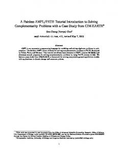
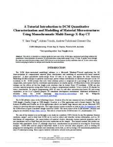
Figure 2 shows the graphical representation of this network.

v2 GoTo Bin

v1

v5

Stop

Work Area

v3 Parts Bin

v4 Leave Bin Figure 2: Network for a Discrete Event System’s State Space The network (V; A) denotes all possible states that a discrete-event system might occupy. Which state a specific system is currently occupying is shown by marking the network. A marked network is the 3-tuple (V; A; µ) where V and A are the network vertices and arcs, respectively. The final element of the triple is a function µ : V ! f0; 1g which associates either zero or one with each vertex of the network (V; A). If µ(v) = 1, then we say vertex v is marked. Otherwise the vertex is unmarked. Graphically, we mark a network by placing a small solid circle (also called a token) in the marked vertex. As shown in figure 2, the vertex v2 is marked. By itself, the marked network (V; A; µ) is an abstract mathematical object. We now bind this object to a specific interpretation so it becomes a model of something. Such a binding is accomplished by labeling the vertices of the network with strings or names that have a concrete meaning. Formally, we denote a labeled marked network by the 4-tuple, (V; A; µ; `) where (V; A; µ) is a marked network and ` : V [ A ! Ω maps the vertices and arcs of the network onto a discrete set of labels. Consider for example, the network shown in figure 2 and let’s introduce the following labeling function on the vertices `(

v1 ) `(v2 )

=

`(

=

`(

=

v3 )

v4 ) `(v5 )

WorkArea GoToBin PartsBin LeaveBin Stopped

=

=

(8) (9) (10) (11) (12)

The labeled vertices are shown in figure 2. With these labels, the network shown in figure 2 provides a graphical model for the computer program we used to control the arms of the vehicle in figure 1. There are, in this figure, 4 discrete states associated with each of the program segments given in the pseudo-code described above. In addition to these 4 states, we’ve also included a fifth state (Stopped) that represents a failure condition under which the system does an emergency stop. 9

As presented so far, the labeled marked network N = (V; A; µ; `) represents the discrete state of the program controlling the arms in the paper’s robot example. We can also, however, introduce a very simple dynamical rule which allows us to view N as a discrete-event dynamical system. Denote the preset and postset of a vertex v as v and v, respectively. Define both of these objects as

v v

= =

fw 2 V fw 2 V

: (w; v) 2 Ag : (v; w) 2 Ag

(13) (14)

The preset (postset) of v therefore consists of all vertices which are connected to v by an input arc , (w; v) (output arc, (v; w)). An arc (w; v) will be said to be enabled if and only if µ(w) = 1. Any enabled arc may fire. Let µ be the network’s marking function before enabled arc (v1 ; v2 ) fires and let µ0 denote the marking function after the arc fires. The relationship between µ and µ0 is

81 < µ0 (w) = : 0µ(w)

if w = v2 if w = v1 otherwise

(15)

In other words, the firing of arc (v1 ; v2 ) unmarks vertex v1 , marks vertex v2 , and leaves all other vertices in the network unchanged. The labeled marked network described above is sometimes referred to as a finite state machine. Finite state machines are often referred to as finite automata. This paper does not distinguish between the two structures. It should be noted that finite automata are usually defined from a language theoretic formulation. To keep the presentation more compact, we treat finite state machines and finite automata in the same way using a graph theoretic formalism. While these models are very useful, it is common practice to augment the structure by labeling the arcs and vertices with statements conditioning the firing of arcs. One common example of such an augmented network is found in logical DES control where finite state machines are augmented with conditional labels that disable the firing of specific arcs of the network as a function of the network’s current marking. When these conditional statements are also functionally related to the states of a continuous-valued dynamical system, then we obtain the Alur-Dill hybrid automaton [1]. The Alur-Dill hybrid automaton was introduced in response to a need to accurately model the behavior of realtime programs. Real-time systems, of course, contain an implicit dynamical system; a clock with associated differential equation x˙ = 1. The clock can be used to condition program execution so that program code segments at executed at the correct real-time, not just in the correct order. Any control systems engineer with experience in the development of embedded control systems will be aware of the use of interval timers in controlling program execution in real-time. The hybrid automata model was introduced to capture this aspect of real-time programming. To formally define the hybrid automaton, we need to introduce the timers and labels mentioned in the opening paragraph of this section. We define the ith timer by the ordered triple xi = ( fi ; xi0 ; ti0 ) where fi : ℜn ! ℜn is a Lipschitz continuous vector field defined over the continuous state space ℜn , xi0 is an initial condition in ℜn , and ti0 is an initial time in ℜ. The timer triple, therefore, can be viewed as an initial value problem and the time of our timer is denoted by the state trajectory, xi (t ) for t  ti0 that satisfies the following initial value problem x˙i xi (ti0 )

= =

fi (x) xi0

(16) (17)

We let X denote a set of timers of the form given above. The set X characterizes the continuous dynamics of our hybrid system. If the vector field f is unity, then we call the timer a clock. The state of the ith timer at time t will be denoted as zi (t ) = (x˙i (t ); xi (t )), i.e. it is defined with respect to the ith timer’s rate and value. 10

In a hybrid automaton, (N ; X ; L ), the labels L tie the discrete and continuous parts of the system together. These labels are mappings from the vertices and arcs of the network N onto formulae in a propositional logic, P , whose truth values are evaluated with respect to the current timer states, z. The logical propositions labeling the network nodes and arcs can be defined in a variety of ways. In this paper we choose the following. We first introduce a set of atomic equations defined over the variables x˙i , xi , xi0 , and fi . Let a and b be real vectors and let c be a real constant, then the basic atomic equations are:



switching equations of the form [x˙i = f j ]. This formula states that the ith timer’s rate is equal to vector field f j ,



guard equations of the form [a0 xi Rb0 x j ] or [a0 xi Rc]. These inequalties mean that the inner product of a and xi , a0 xi , stands in relation R (either < or >) to b0 x j or real constant c.



reset equations of the form [a0 xi0 = c] which means that a0 xi is equal to real constant c.

Legal formulae in P are defined inductively by the following rules:

  

Any atomic equation is in P , If p and q are in P then [ p ^ q] is in P if p is in P then˜p is in P .

The preceding paragraph defined the syntax for formulae in P . The meaning or interpretation of these formulae is made with respect to the timer states z = (x˙; x). In particular, we say that an atomic formula is satisfied by timer state z(t ) = (x˙(t ); x(t )) if and only if the equation is true when evaluated with respect to those states at time t. The formula p ^ q is true if both p and q are true under the given timer states. The formula ˜p is true if p is not true under the current timer states. The current timer state is said to satisfy a formulae p 2 P if and only if it has the truth value of true. The labeling function L associates each vertex and arc of the network with a proposition in P . The bindings implied by L determine how the continuous and discrete parts of our hybrid system interact. For hybrid automata, this interaction is defined according to the following rules:

 

The network arcs are labeled with equations in P formed from guard atomic equations, [a0 xi Rc] or [a0 xi Rb0 x j ]. These conditions on the arcs represent additional enabling conditions for an arc’s firing. Recall that an arc ((w; v)) of a network may only fire if vertex w is marked. In the hybrid automaton, this same arc may fire at time t if and only if vertex w is marked and L ((w; v)) is true at time t. The network vertices are labeled with formulae whose atomic equations are switching or reset equations. These formulae are interpreted as follows. If the formulae do not evaluate to true when the vertex is first marked , then the timer states will be reset to make these predicates true. In the case of the reset equations, this means that the clock time, x is reset to the specified value. For switching equations, the timer’s rate, x˙ is set to the specified vector field. We therefore see that these reset/switching conditions allow the hybrid automaton to model autonomous jumping and switching behaviors.

There are several important classes of hybrid automata. When the timers are chosen to be clocks, then we obtain the class of linear hybrid automata. Timed automata are linear hybrid automata whose guard 11

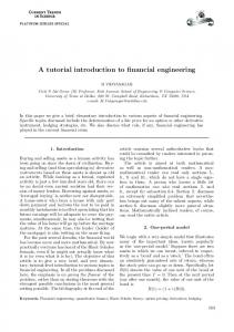
conditions define rectangles in the continuous state space. The class of rectangular hybrid automata occur when the timers are represented as rectangular differential inclusions of the form x˙ 2 [a; b] and the guard conditions also define rectangular sets. The system whose continuous dynamics are illustrated in figure 1 and whose discrete dynamics are illustrated in figure 2 can be easily modeled using a hybrid automaton. The resulting hybrid automaton is shown in figure 3. In this automaton, we see that the vertex label WorkArea has no predicate associated with it. The arc, however, between WorkArea and GoToBin is labeled with the conditional formula ˜ [x > 0]. In other words when the lock variable x is no longer nonzero this arc may fire and the system will switch to the logical state GoToBin. Go To Bin

Go To Bin

..

~[x>0]

θ1 = θ1 - T

|θ1+ θB| < 0.1

..

x=1

θ 2= θ2 - T

~[x>0]

|θ2+ θB| < 0.1

x=1

-10 < θ1< 100

-10 < θ1< 100

..

θ1 = θ1 θ2 = θ2 Work Area

|θ1+ θ B- π/2 | < 0.1

-10 < θ1< 100

x=0

..

θ1 = θ1

..

θ1 = θ1 + T

..

..

θ2 = θ2

..

θ 2= θ2 + T

Parts Bin Work Area

|θ1+ θB| > 0.1

-10 < θ1< 100

x=0

|π/2 - θ2- θB| < 0.1

Parts Bin

|π/2 - θ2- θB| > 0.1

Leave Bin

Leave Bin

Figure 3: Hybrid Automaton for Robotic System The discrete state GoToBin is labeled with the predicate [x = 1] ^ [θ¨ 1 = θ˙ 1 + k(θ1 + θb )] This predicate sets the lock variable to 1 thereby indicating to arm 2 that it is heading towards the parts bin. While in this state, the system also sets its timer rate θ¨ 1 to the vector field which begins moving the arm towards the parts bin. The arc connecting GoToBin to the discrete state PartsBin is labeled with the conditional predicate [θ¯ 21 100θ¯ 22 ] < 0]. This conditional predicate is a indefinite quadratic form representing a conic sector enclosing the parts bin. Also note that the transition out of discrete state GoToBin has a nondeterministic next state in the sense that we can either transition to PartsBin or Stopped. The condition for transitioning to the Stopped state is [θ1 > 100] _ [θ1 < 10] This is a safety condition which is triggered if the arm moves too far (i.e. hits its physical stops). In this case, we transition to the Stopped state. The Stopped state is a deadlocked state from which all forward progress in the system ceases. It is labeled by a predicate which turns off the system, so it is labeled with the predicate [θ¨ 1 = θ1 ] ^ [θ¨ 2 = θ2 ] thereby causing both arms to eventually stop their motion. Once in the parts bin, the system begins moving the arm out of the bin. Therefore the state PartsBin is labeled with the predicate [θ¨ 1 = θ˙ 1 + k(θ1 + θb π=2)] Once the arm is out of the bin, we allow the system’s discrete state to transition to the state LeaveBin. The predicate guarding this transition is [θ¯ 21 100θ¯ 2] > 0. Upon leaving the bin, the system resets the lock variable so the other arm can access the parts bin, hence

12

the predicate on LeaveBin is [x = 0]. Finally, the system returns to the WorkArea state if the appropriate conditions on the angle are satisfied or exits to the Stopped state if the limit conditions on the arm’s angular position are violated. Note that the preceding discussion stepped through the different discrete states of the automaton controlling the first arm of the vehicle. A similar automaton shown in figure 3 is also used to control the second arm of the vehicle. The coupling between these two discrete structures is through the lock variable, x and the body angle θb .

5 System Specifications Control theoretic measures of system performance are frequently taken to be the size of some important signal within the control system’s feedback loop. Signal size is measured using a functional that maps each signal (function) onto a positive real number. Common measures of signal size include signal energy, power, and amplitude. In a more abstract setting these measures are referred to as signal norms and norm-based measures of system performance represent the starting point for most optimal controller design methods. In practice, however, a single norm based measure of performance is rarely adequate to completely characterize what the designer wants the system to do. It may, for example, be necessary to condition system performance on the system’s reference signal. A gain scheduled system may need to satisfy one norm bound specification at one of its setpoints and yet this specification may be relaxed at another setpoint without hurting the system’s ability to satisfactorily meet specified performance goals. Finally, it should be noted that norm based performance measures are clearly inappropriate for supervised systems such as the system in figure 1. In this case, the mutual exclusion requirement is a high level behavioral constraint which is not easily expressed in terms of a signal with bounded norm. The conclusion that must be drawn from the preceding observations is that while traditional control theoretic performance measures are valuable, they do not provide sufficient flexibility to characterize the wide range of desired behaviors our systems need to satisfy. To meet these more complex and realistic system specifications it is imperative that a more expressive method be adopted for capturing the designer’s requirements. Formal logics can be used to express more complex system specifications. We’ve already used a propositon logic to characterize the labels for a hybrid automaton. We now turn to the use of formal logics, and in particular temporal logic, to express requirements on desired system behavior. A logic may be characterized by three things, its atomic formulae, its syntax and its semantics. The atomic formulae are a set of elementary formulae or equations. The syntax of the logic is the set of rules defining how atomic formulae may be combined to form legal formulae or predicates in the logic. The semantics characterize the meaning of the logical predicates with respect to a specified frame. The frame is a set of states through which a system might evolve (i.e. our hybrid automaton). The meaning of logical formulae is then determined by defining the truth values of all logical equations with respect to the frame states. In particular, if a logical formula, p, is true with respect to the frame state s, then we say that s satisfies p and we denote this as s j=F p where F is the frame on which s is defined. In cases where the frame is clear, we will drop the subscript F. In temporal logics, the frame states can be ordered (i.e. with respect to order of occurrence) and this allows us to introduce and reason about several notions of time. A linear temporal logic assumes all states are strictly ordered and hence allows us to reason about purely deterministic strings of events. A branching

13

temporal logic assumes all frame states are partially ordered and allows us to reason about systems with nondeterministic dynamics. In our case, we will look at system specifications that can be expressed as formulae in a branching temporal logic since hybrid systems are usually nondeterministic. We refer to this logic as CTL1. It is a subset of the well-known computation tree logic (CTL). Before defining the atomic propositions, syntax and semantics of our specification logic, we need to introduce some preliminary notation. Consider the hybrid automaton, H = (N ; X ; L ). The hybrid state of the system at time t is denoted as σ(t ) = (x(t ); µ(t )) where x(t ) is the continuous-valued state trajectory and µ(t ) is the network marking history (as a function of time). We define the event projection πe (σ(t )) by the equation πe (σ(t )) = µ(t1 ); µ(t2 );


; µ(tn );




(18)

In other words, the event projection of σ(t ) is a sequence of discrete network states in which no two adjacent states are the same. The event projection πe (σ) is sometimes called the trace of the hybrid trajectory. Let σ(t ) be a hybrid system trajectory, then the atomic formulae for our specification logic take the form, [a0 x(t ) > b] or [µ(t ) = µ0 ]. The first atomic formula is the conditional formula used earlier as a guard condition in the hybrid automaton. The current hybrid state σ is said to satisfy this atomic formula if the inequality is true for the given state at time t. The second atomic formula is a specific marking of the network. In this case, the hybrid state at time t satisfies the predicate if and only if the network’s trace at time t equals µ. The syntax of a logic is a set of fundamental legal formulas. These fundamental formulas provide a way of inductively defining all legal formulas in CTL1. In our case, the syntax is as follows.

    

p is in CTL1 if p is atomic if p is in CTL1 then˜p is in CTL1 if p and q are in CTL1 then p ^ q is in CTL1.

if p and q are in CTL1 then p9U q is in CTL1, if p and q are in CTL1 then p8U q is in CTL1

The formula 8U p and 9U p are equivalent to [true]8U p and [true]9U p, respectively. The notation above may seem confusing, but essentially, we are assuming that all legal formulas in CTL1 can be expressed as either a predicate, p, a predicate with a unary operator, (i.e. ˜ p, 8U p, 9U p) or a binary operation on legal predicates, (i.e. p ^ q, p8U q, p9U q). Note that 8U and 9U represent binary or unary operators on predicates. These formulas provide a way of building up more complex formulas. Therefore the formula p _ [q8U r] is legal because p and [q8U r] are both legal predicates according to the syntactical rules given above. The preceding syntactical formulas represent a set of abstract formulas but provide no interpretation or meaning to these formulas. The interpretation of the formulas is determined by the logic’s semantics. The semantics of CTL1 are defined with respect to a hybrid state, s. Let σ(t ) = (x(t ); µ(t )) be a hybrid trajectory generated by the hybrid automaton, (N ; X ; L ). As the frame is given, we drop explicit mention of it in the formulae. The meaning of the generating CTL1 formulae is as follows: s j= p

s j= ˜p s j= p ^ q

, , ,

p is satisfied by state s

(19)

p is not satisfied by state s p and q are satisfied at state s

(20) (21) 14

s j= p9U q

,

s j= p8U q

,

there exists a hybrid trajectory σ(t ) such that σ(0) = s and a time t1 such that

(22)

σ(t ) j= p _ q for t < t1 and σ(t1 ) j= q.

(25)

(23) σ(t ) j= p _ q for t < t1 and σ(t1 ) j= q. for all hybrid trajectories σ(t ) such that σ(0) = s, there exists a time t1 such that (24)

We therefore see that the formula p _ q represents our usual notion of logical conjunction where as ˜ p represent the logical not operation. The other two formulae p8U q and p9U q have a special meaning which is specific to temporal logics. These operators provide a way of describing temporal relationships between predicates. The formula p8U q can be seen as saying that for all hybrid trajectories, predicate p is true until predicate q is true. The formula p9U q is the other existential formula meaning that there exists a trajectory in which p is true until q is true. CTL1 allows us to express complex specifications relating the discrete and continuous states of the hybrid system. It should be noted that we’ve made no attempt in this paper to construct a complete logic. More powerful temporal logics using the hybrid automaton as a frame will be found in [20] and [21]. CTL1, as introduced in this paper, is only intended as a pedagogical tool illustrating some of the basic concepts encountered in using temporal logics to express specifications for hybrid dynamical systems. In the remainder of this section we present some specific examples illustrating the use of CTL1 in specifying acceptable behaviors for the robotic system illustrated in figure 1. In referring to the example in figure 1, the first requirement is that the system must satisfy a mutual exclusion requirement. A temporal logic specification capturing this desired constraint is,

8U˜˜ [PartsBin1 ^ PartsBin2 ]

(26)

This particular specification equation says that for all possible traces, the computer programs controlling both arms will not enter their critical sections at the same time. This mutual exclusion requirement, however, is only on the discrete part of the system and does not necessarily capture the true constraint we’re interested in. A more realistic constraint on the system would be expressed as follows:

8U˜ [[jθ1 + θbj