A tutorial on KAM theory Rafael de la Llave Department of Mathematics, The University of Texas at Austin, Austin, TX 78712-1082 E-mail address:
[email protected]
1991 Mathematics Subject Classification. Primary 37J40, 70K43 Secondary: 37J45, 70K60; Key words and phrases. KAM theory, stability, Perturbation theory,quasiperiodic orbits,Hamiltonian systems Abstract. This is a tutorial on some of the main ideas in KAM theory. The goal is to present the background and to explain and compare somewhat informally some of the main methods of proof. It is an expanded version of the lectures given by the author in the Summer Research Institute on Smooth Ergodic Theory Seattle, 1999. The style is somewhat informal and expository and it only aims to be an introduction to the primary literature. It does not aim to be a systematic survey nor to present full proofs.
Contents Preface
iii
Introduction Acknowledgements
1 3
Chapter 1. Some Motivating Examples 1.1. Lindstedt series for twist maps 1.2. Siegel disks
5 5 15
Chapter 2. Preliminaries 2.1. Quasi-periodic functions 2.2. Preliminaries in analysis 2.3. Regularity of functions defined in closed sets. The Whitney extension theorem 2.4. Diophantine properties 2.5. Estimates for the linearized equation 2.6. Geometric structures 2.6.1. Symplectic and volume preserving geometry 2.6.2. Sketch of the proof of Darboux Theorem 2.6.3. Reversible systems 2.7. Canonical perturbation theory 2.8. Generating functions
23 24 25
Chapter 3.
Two KAM Proofs in a Model Problem
67
Chapter 4.
Hard Implicit Function Theorems
83
31 33 37 43 43 52 53 54 64
Chapter 5. Persistence of Invariant Tori for Quasi-integrable Systems 101 5.1. Kolmogorov’s method 102 5.2. Arnol’d method 111 5.3. Lagrangian proof 117 5.4. Proof without changes of variables 121 5.5. Some criteria to organize and compare KAM proofs 130 Chapter 6.
Aubry-Mather Theory
135
Chapter 7.
Some Remarks on Computer Assisted Proofs
147
Chapter 8.
Some Recent Developments
153
i
ii
CONTENTS
8.1. 8.2. 8.3. 8.4. 8.5. 8.6. 8.7. 8.8. 8.9. 8.10. 8.11. 8.12. 8.13. 8.14. 8.15. 8.16.
Lack of parameters Volume preserving Infinite dimensional systems Systems with local couplings Non-degeneracy conditions Weak KAM Reducibility Spectral properties of Sch¨odinger operators Higher dimensional tori Elliptic PDE Renormalization group Rotations of the circle More constructive proofs and relations with applications The limits of validity of the theory Methods based on direct compensations of series Related subjects: averaging, adiabatic invariants
Bibliography
153 153 153 154 154 154 154 155 155 155 156 156 157 157 157 158 161
Preface This is an slightly edited version of [dlL01]. Almost no new material has been added. This is mainly because the author could not undertake these additions. We have eliminated some typos and mistakes, added some explanations and included proofs or sketches of proofs of several standard results and a few new sections. Regretfully, we could not include an adequate treatment of several important topics such as the application of KAM in celestial mechanics, renormalization group and a discussion of the boundary of validity of KAM or some of the most sophisticated modern proofs. Again, we want to emphasize that this is a tutorial. It is meant to be read in an active way, completing the sketches of proof presented here (we make no claims about the proofs being complete), working out the exercises included in the text (some of them are gaps in the literature, whose solution, I think would be quite welcome as a good master or undergraduate thesis) fixing the occasional typo or bad expression (the author would love to hear about them!) or reading the original literature (we make no claim of originality for this manuscript, which is certainly not a substitute for the original papers on which it is based). The only justification of writing this book is that it can encourage people to read different papers in the original literature and compare them. I certainly thank to the people who made suggestions on the material both in the preparation of the first version and in the revision of the material (see subsection “Acknowledgements” at the end of Introduction).
iii
Introduction The goal of these lectures is to present an introduction to some of the main ideas involved in KAM theory on the persistence of quasiperiodic motions under perturbations. The name comes from the initials of A. N. Kolmogorov, V. I. Arnol’d and J. Moser who initiated the theory. See [Kol54], [Arn63a], [Arn63b], [Mos62], [Mos66b], [Mos66a] for the original papers. By now, it is a full fledged theory and it provides a systematic tool for the analysis of many dynamical systems and it also has relations with other areas of analysis. The conclusions of the theory are, roughly, that in C k – k rather high depending on the dimension – open sets of of dynamical systems satisfying some geometric properties – e.g., Hamiltonian, volume preserving, reversible, etc. – there are sets of positive measure covered by invariant tori (these tori are the image of a quasi-periodic motion). In particular, since sets with a positive measure of invariant tori is incompatible with ergodicity, we conclude that for the systems mentioned above, ergodicity cannot be a C k generic property [MM74]. Of course, the existence of the quasiperiodic orbits, has many other consequences besides preventing ergodicity. The invariant tori are important landmarks that organize the motion of the system. Notably, many of the mechanisms of instability use as ingredients some invariant tori. Besides its applications to mechanics, dynamical systems and ergodic theory, KAM theory has grown enormously and has very interesting ramifications in dynamical systems and in analysis. In dynamical systems, we will mention that KAM theory is closely related to averaging theory and Nekhoroshev’s effective stability results (See [DG96] for a unified exposition of KAM and Nekhoroshev theory) and, conversely, KAM theory is related to the theory of instabilities (sometimes called Arnol’d diffusion). Also, KAM theory shows that for C r open sets of Hamiltonians – r large – the ergodic hypothesis is false. See [MM74]. On the side of more analytical developments, KAM theory is connected to very sophisticated and powerful theorems in functional analysis that can be used to solve a variety of functional equations, many of which have interest in ergodic theory and in related disciplines such as differential geometry. There already exist excellent surveys, systematic expositions and tutorials of KAM theory. 1
2
INTRODUCTION
We quote, in (more or less) chronological order, the following: [Arn63b], [Mos66b], [Mos66a], [Mos67], [AA68], [R¨ us70], [R¨ us], [Mos73], [Zeh75], [Zeh76a], [P¨ os82], [Gal83a], [Dou82a], [Bos86], [Sal86], [Gal86], [P¨ os92] [Yoc92], [AKN93], [dlL93], [BHS96b], [Way96], [R¨ us98], [Mar00], [P¨ os01], and [Chi03]. Hence, one has to justify the effort in writing and reading yet another exposition. I decided that each of the surveys above has picked up a particular point of view and tried to either present a large part of KAM theory from this point of view or to provide a particularly enlightening example. Given the high quality of all (but one) of the above surveys and tutorials, there seems to be little point in trying to achieve the same goals. Therefore, rather than presenting a point of view with full proofs, this tutorial will have only the more modest goal of summarizing some of the main ideas entering into KAM theory and describing and comparing the main points of view. This booklet certainly does not aim to be a substitute for the above references. On the contrary, the more modest goal is to serve as a small guide of what the interesting reader may find. The reader who wants to learn KAM theory is encouraged to read the papers above. One of the disadvantages of covering such wide ground is that the presentation will have to be sketchy at some points. Hopefully, we have flagged a good fraction of these sketchy points and referred to the relevant literature. I would be happy if these lectures provide a road map (necessarily omitting important details) of a fraction of the literature that encourages somebody to enter into the field. Needless to say, this is not a survey and we have not made any attempt to be systematic nor to reach the forefront of research. It should be kept in mind that KAM theory has experienced spectacular progress in recent years and that it is a very active area of research. See Chapter 8 for an – incomplete! – glimpse on what has been going on. Needless to say in this tutorial, we cannot hope to do justice to all the topics above. (Indeed, I have little hope that the above list of topics and references is complete.) The only goal is to provide an entry point to the main ideas that will need to be read from the literature and, possibly, to convey some of the excitement and the beauty of this area of research. Clearly, I cannot (and I do not) make any claim of originality or completeness. This is not a systematic survey of topics of current research. The modest goal I set set for these notes is to help some readers to get started in the beautiful and active subject of KAM theory by giving a crude road map. I just hope that the many deficiencies of this tutorial will incense somebody into writing a proper review or a better tutorial. In the mean time, I will be happy to receive comments, corrections and suggestions for improvement of this tutorial which will be made available electronically in MP ARC. In spite of the fact that KAM theory has a reputation of being difficult, it is my experience that once one can read one or two papers and work out the details by oneself, reading subsequent papers is very easy. A well written
INTRODUCTION
3
paper rather than launching into technicalities, often has early in the paper a short summary of what are the important new ideas. Often a moderate expert can finish the proofs better than the author. In order to facilitate this active learning, I have suggested some exercises along the proofs. (Perhaps the best exercise would be to write better notes than the ones here.) Acknowledgements. The work of the author was supported in part by NSF grants and, during Spring 2003 by a Dean’s Fellowship at U. T. The participation of the AMS SRI Smooth ergodic theory and its applications in Seattle 1999 was seminal in getting a first version of this tutorial. The enthusiasm of the participants and organizers of the SRI was extremely stimulating. I received substantial assistance in the preparation of the notes for the SRI from A. Haro, N. Petrov, J. Vano. Comments from H. Eliasson, T. Gramchev, and many other participants ` Jorba, M. Sevryuk, R. Perez-Marco shortly afterwards in the SRI and by A. removed many mistakes and typos. Needless to say, the merit of all the surviving mistakes belongs exclusively to the author. In the revision of the material after [dlL01] was published, I have benefited from comments and encouragement from many individuals. In alphabetical order, D. Damjanovic, M. Levi, J. Vano, N. Petrov, Special thanks to A. Haro and the participants in a reading seminar in Barcelona, to D. Treschev, who supervised a translation into Russian, and to A. Gonz´alez. I also tried some of the material on the participants of the Working seminar on Dynamical Systems at U.T. Austin and in the X Jornadas de Verano at CIMAT (Guanajuato). Parts of this work are based on unpublished joint work with other people that we intend to publish in fuller versions. Thanks also to the AMS staff who participated in the preparation of the SRI.
CHAPTER 1
Some Motivating Examples 1.1. Lindstedt series for twist maps One of the original motivations of KAM theory was the study of quasiperiodic solutions of Hamiltonian systems. In this Chapter we will cover some elementary and well-known examples. One particularly motivating example is the so-called standard map.1 The standard map is a map from R × T to itself. We denote the real coordinate by p and the angle one by q. Denoting by pn , qn the values of these coordinates at the discrete time n, the map can be written as: (1.1)
pn+1 = pn − εV 0 (qn )
qn+1 = (qn + pn+1 ) mod 1,
where V (q) = V (q+1) is a smooth (for the purposes of this section, analytic) periodic function. We will also use a more explicit expression for the map. (1.2)
¡ ¢ Tε (p, q) = p − εV 0 (q), q + p − εV 0 (q) .
Substituting the expression for pn+1 given in the second equation of (1.1) into the first, we see that the system (1.1) is equivalent to the second order equation. (1.3)
qn+1 + qn−1 − 2qn = −εV 0 (qn ),
The first, “Hamiltonian”, formulation (1.1) appears naturally in some mechanical systems (e.g., the kicked pendulum). The second, “Lagrangian”, one (1.3) appears naturally from a variational principle, namely, it is equivalent to the equations (1.4)
∂L/∂qn = 0
with (1.5)
L(q) = −
X ·1 n
2
¸ (qn+1 − qn − a) + εV (qn ) . 2
1We will use the same example as motivation in Section 5.3 and in Chapter 6. We hope that studying the same model by different methods will illustrate the relation between the different approaches. 5
6
1. SOME MOTIVATING EXAMPLES
The equations (1.4) – often called Euler-Lagrange equations – express that {qn } is a critical point for the action (1.5). The model (1.5) has appeared in solid state physics under the name Frenkel-Kontorova model (see, e.g., [ALD83]). One physical interpretation (not the only possible one) that has lead to many heuristic insights is that qn is the position of the nth atom in a chain. These atoms interact with their nearest neighbors by the quadratic potential energy 21 (qn+1 − qn − a)2 (corresponding to springs connecting the nearest neighbors) and with a substratum by the potential energy εV (qn ). The parameter a is the equilibrium length of each spring. Note that a drops from the equilibrium equations (1.3) but affects which among all the equilibria corresponds to a minimum of the energy. Another interpretation, of more interest for the theme of these lectures, is that qn are the positions at consecutive times of P a one-degree of freedom twist map. The action of the trajectory is L = i L(qi , qi+1 ) The general term in the sum L(qi , qi+1 ) is the generating function of the map. (See Chapter 2.8.) Then, the Euler-Lagrange equations for critical points of the functional are equivalent to the sequence {qn } being the projection of an orbit. The first formulation (1.1) is area preserving whenever V 0 is a periodic function of the cylinder – not necessarily the derivative of a periodic function (i.e., the Jacobian of the transformation (pn , qn ) 7→ (pn+1 , qn+1 ) is equal to 1). When, as we have indicated, V 0 is indeed the derivative of a periodic function, then the map is exact, a concept that we will discuss in greater detail in Chapter 2.6 and that has great importance for KAM theory. If we look at the map (1.1) for ε = 0, we note that it becomes
(1.6)
pn+1 = pn , qn+1 = qn + pn ,
so that the “horizontal” circles {pn = const, n ∈ Z} in the cylinder are preserved and the motion of each qn in each circle is a rigid rotation that is faster in the circles with larger pn . Note that when p0 is an irrational number, a classical elementary theorem in number theory shows that the orbit is dense on the circle. (A deeper theorem due to Weyl shows that it is actually equidistributed in the circle.) We are interested in finding whether, when we turn on the perturbation ε, some of this behavior persists. More concretely, we are interested in knowing whether there are quasi-periodic orbits that persist and that fill a circle densely. Problems that are qualitatively similar to (1.1) appear in celestial mechanics [SM95] and the role of these quasi-periodic orbits have been appreciated for many years. One can already find a rather systematic study in [Poi93] and the treatment there refers to many older works.
1.1. LINDSTEDT SERIES FOR TWIST MAPS
7
T(γ)
-
+ γ
Figure 1. The flux is the oriented area between a circle and its image. We note that the existence of quasi-periodic orbits is hopeless if one allows general perturbations of (1.6). For example, if we take a map of the form (1.7)
pn+1 = pn − εpn , qn+1 = qn + pn+1 ,
we see that applying repeatedly (1.7), we have pn = (1 − ε)n p0
so that, when 0 < ε < 2, all orbits concentrate on the very small set p = 0 and that we get at most only one frequency. When ε < 0 or ε > 2, all the orbits except those in p = 0, blow up to infinity. Hence, we can have maps with radically different dynamical behavior by making arbitrarily small perturbations. More subtly, the orbits of (1.8)
pn+1 = pn + ε, qn+1 = qn + pn+1
escape towards infinity and never come back to themselves (in particular, can never be quasi-periodic). The first example is not area preserving and the motion is concentrated in a smaller area (in particular, it does not come back to itself). The second example is area preserving but has non-zero “flux”. Definition 1.1. The “flux” of an area preserving map T of the cylinder is defined as follows: given a continuous circle γ on the cylinder, the flux of T is the oriented area between T (γ), the image of the circle, and γ — see Figure 1. The fact that the map is area preserving implies easily that this flux is independent of the circle (hence it is an invariant of the map). Clearly, if the map T had a continuous invariant circle, the flux should be zero, so we cannot find an invariant circle in (1.8) for ε 6= 0 since the flux is ε.
8
1. SOME MOTIVATING EXAMPLES
Remark 1.2. If a map has a homotopically nontrivial invariant curve, then the flux is zero (compute it for the curve). Conversely, if the flux is zero, any homotopically non-trivial curve has to have an intersection with its image. (If it did not have any intersection, by Rolle’s theorem, then the image would always be in above or below the curve.) The property that every curve intersects its image plays an important role in KAM theory and is sometimes called intersection property. Besides area preserving and zero flux, there are other geometric assumptions that imply the intersection property. Moreover, there are other properties that imply that one can proceed with the iteration because the undesired terms do not appear. One notable example is the reversibility property, which appears naturally in many physical systems (e.g., all circuits with capacitances and inductances but no resistance). The KAM theorem for reversible mappings is carried out in great detail in [Sev86], [BHS96b]. The paper [P¨ os82] devotes one section to the proof of KAM theorem for reversible systems. For information about reversible systems in general – in particular for examples of reversible systems without intersection property – see also [AS86]. As a simple calculation shows, that perturbation in (1.1) is of the form R1 V n ), with V 1-periodic — therefore 0 V 0 (qn ) dqn = V (1) − V (0) = 0 — the flux of (1.1) is zero. We see that even the possibility that there exist these quasi-periodic orbits filling an invariant circle depends on geometric invariants. Indeed, when we consider higher dimensional mechanical systems, the analogue of area preservation is the preservation of a symplectic form, the analogue of the flux is the Calabi invariant [Cal70] and the systems with zero Calabi invariant are called exact. We point out, however, that the relation of the geometry to KAM theory is somewhat subtle. Even if the above considerations show that some amount of geometry is necessary, they by no means show what the geometric structure is, and much less hint on how it is to be incorporated in the proof. The first widely used and generally applicable method to study numerically quasi-periodic orbits seems to have been the method of Lindstedt. (We follow in this exposition [FdlL92a].) The basic idea of Lindstedt’s method is to consider a family of quasiperiodic functions depending on the parameter ε and to impose that it becomes a solution of our equations of motion. The resulting equation is solved – in the sense of power series in ε – by equating terms with same powers of ε on both sides of the equation. We will see how to apply this procedure to (1.1) or (1.3). In the Hamiltonian formulation (1.1), (1.2) we seek Kε : T1 → R × R1 in such a way that 0 (q
(1.9)
Tε ◦ Kε (θ) = Kε (θ + ω).
1.1. LINDSTEDT SERIES FOR TWIST MAPS
9
We set (1.10)
Kε (θ) =
∞ X
εn Kn (θ)
n=0
and try to solve by matching powers of ε on both sides of (1.9), (after expanding Tε ◦ Kε (θ) as much as possible in ε using the Taylor’s theorem).2 That is, Tε ◦ Kε (θ) = T0 ◦ K0 + ε[T1 ◦ K0 + (DT0 ◦ K0 )K1 ]
+ε2 [T2 ◦ K0 + (DT0 ◦ K0 )K2 1 +(DT1 ◦ K0 )K1 + (D2 T0 ◦ K0 )K1⊗2 ] + . . . . 2 In the Lagrangian formulation (1.3) we seek gε : R → R satisfying gε (θ + 1) = gε (θ) + 1
— or, equivalently, gε (θ) = θ + `ε (θ) with `ε (θ + 1) = `ε (θ), i.e., `ε : T1 → T1 — in such a way that (1.11)
`ε (θ + ω) + `ε (θ − ω) − 2`ε (θ) = −εV 0 (θ + `ε (θ)).
If we find solutions of (1.11), we can ensure that some orbits qn solving (1.3) can be written as qn = nω + `ε (nω). Note that the fact that, when we choose coordinates on the circle, we can put the origin at any place, implies that Kε (· + σ) is a solution of (1.9) if Kε is, and that `ε (· + σ) + σ is a solution of (1.11) if `ε is. Hence, we can – and will – always assume that Z 1 (1.12) `ε (θ) dθ = 0. 0
This assumption, will not interfere with existence questions, since it can always be adjusted, but will ensure uniqueness. We first investigate the existence of solutions of (1.11) in the sense of formal power series in ε. If we write 3 ∞ X `n (θ)εn `ε (θ) = n=0
and start matching powers of ε in (1.11), we see that matching the zero order terms yields 2The notation is somewhat unfortunate since K could mean both the n term in the n
Taylor expansion and Kε evaluated for ε = n. In the discussion that follows, K1 ,K2 , etc. will always refer to the Taylor expansion. Note that K0 is the same in both meanings. 3The same remark about the unfortunate notation we made in (1.10) also applies here.
10
(1.13)
1. SOME MOTIVATING EXAMPLES
Lω `0 (θ) ≡ `0 (θ + ω) + `0 (θ − ω) − 2`0 (θ) = 0, Z 1 `0 (θ) dθ = 0. 0
The operator Lω (1.13), which will appear repeatedly in KAM theory, can be conveniently analyzed by using Fourier coefficients. Note that Lω e2πikθ = 2(cos 2πkω − 1) e2πikθ .
Hence, if η(θ) =
ˆk e2πikθ , kη
P
then the equation Lω ϕ(θ) = η(θ)
reduces formally to 2(cos 2πkω − 1) ϕˆk = ηˆk .
We see that if ω ∈ / Q, the equation (1.13) can be solved formally in Fourier coefficients and `0 = 0. (Later we will develop an analytic theory and describe precisely conditions under which these solutions can indeed be interpreted as functions.) When ω ∈ / Q, we see that cos 2πkω 6= 1 except when k = 0. Hence, even to write a solution we need ηˆ0 = 0, and then we can write the formal solutions as (1.14)
ϕˆk =
ηˆk , 2(cos 2πkω − 1)
k 6= 0.
Note, however, that the status of the solution (1.14) is somewhat complicated since 2πkω is dense on the circle and, hence, the denominator in (1.14) becomes arbitrarily small. Nevertheless, provided that η is a trigonometric polynomial (see Exercise 1.6, where this is established under certain circumstances) and ω is irrational, the formal solution (1.14) is also a trigonometric polynomial. When the R.H.S. is analytic and the number ω satisfies certain number theoretic properties that ensure that the denominator does not become too small (this properties, which appear motivated here, will be the main topic in Section 2.4, it is possible to show that the solution is also analytic. (See Exercise 1.16.) The equation obtained by matching ε1 is (1.15)
Lω `1 (θ) = −V 0 (θ);
Z
1
`1 (θ) dθ = 0. 0
R1 Since 0 V 0 (θ) dθ = 0, we see that (1.15) admits a formal solution. (Again, R1 we note that the fact that 0 V 0 (θ) dθ = 0 has a geometric interpretation as zero flux.) Matching the ε2 terms, we obtain
1.1. LINDSTEDT SERIES FOR TWIST MAPS
(1.16)
Z
Lω `2 (θ) = −V 00 (θ)`1 (θ);
11
1
`2 (θ) dθ = 0, 0
and, more generally,
(1.17)
Z
Lω `n (θ) = Sn (θ);
1
`n (θ) dθ = 0, 0
where Sn is an expression which involves derivatives of V and terms previously computed. It is true (but by no means obvious) that Z 1 Sn (θ) dθ = 0, (1.18) 0
so that we can solve (1.17) and proceed to compute the series to all orders (when ω is irrational and S is a trigonometric polynomial or when ω is Diophantine (see later) and S is analytic). The fact that (1.18) holds was already pointed out in Vol. II of [Poi93]. We will establish (1.18) directly by a seemingly miraculous calculation, whose meaning will become clear when we study the geometry of the problem. (We hope that going through the messy calculation first will give an appreciation for the geometric methods. Similar calculations will appear in Chapter 5.3.) [