Typeset in LATEX 2ε using AMS-LATEX 2.0 using gsm-l document class. ISBN 952-92-0339-X ..... noticed that Eliasson's method could be performed using the same diagrams that physicists had been using since Feynman. Namely one can ...
Renormalization methods in KAM theory
Emiliano De Simone
FACULTY OF S CIENCE D EPARTMENT OF M ATHEMATICS AND S TATISTICS U NIVERSITY OF H ELSINKI 2006
2000 Mathematics Subject Classification. Primary 37J40; Secondary 70H08, 11D75, 11D75 Key words and phrases. KAM, small divisors, diophantine, Renormalization Group
A BSTRACT. It is well known that an integrable (in the sense of ArnoldJost) Hamiltonian system gives rise to quasi-periodic motion with trajectories running on invariant tori. These tori foliate the whole phase space. If we perturb an integrable system, the Kolmogorow-ArnoldMoser (KAM) theorem states that, provided some non-degeneracy condition and that the perturbation is sufficiently small, most of the invariant tori carrying quasi-periodic motion persist, getting only slightly deformed. The measure of the persisting invariant tori is large together with the inverse of the size of the perturbation. In the first part of the thesis we shall use a Renormalization Group (RG) scheme in order to prove the classical KAM result in the case of a non analytic perturbation (the latter will only be assumed to have continuous derivatives up to a sufficiently large order). We shall proceed by solving a sequence of problems in which the perturbations are analytic approximations of the original one. We will finally show that the approximate solutions will converge to a differentiable solution of our original problem. In the second part we will use an RG scheme using continuous scales, so that instead of solving an iterative equation as in the classical RG KAM, we will end up solving a partial differential equation. This will allow us to reduce the complications of treating a sequence of iterative equations to the use of the Banach fixed point theorem in a suitable Banach space.
iii
Typeset in LATEX 2ε using AMS -LATEX 2.0 using gsm-l document class.
ISBN 952-92-0339-X (paperback) ISBN 952-10-3129-8 (PDF) http://ethesis.helsinki.fi/ Otamedia Oy Espoo 2006
Contents
Acknowledgements Chapter 1.
Introduction
vii 3
§1.
The KAM problem
5
§2.
The "Lindstedt series" and the first KAM proofs
8
§3.
Inside the Lindstedt series
10
Part 1. Differentiable perturbation Chapter 2. §1.
The KAM theorem and RG scheme
Scheme
Chapter 3.
Setup and preliminary results
15 16 23
§1.
Spaces
23
§2.
A priori bounds for the approximated problems
25
§3.
Cauchy Estimates
29
§4.
The Cutoff and n-dependent spaces
30
§5.
n-dependent bounds
32
Chapter 4.
The Ward identities (revised)
37 v
vi
Contents
§1.
Resonances and compensations
Chapter 5.
The Main Proposition
40 43
§1.
Proof of (a)
44
§2.
Proof of (b)
47
§3.
Proof of (c)
49
Chapter 6.
Proof of Theorem 1
59
Part 2. Continuous Renormalization Chapter 7.
Introduction and continuous RG scheme
65
§1.
The continuous scales
66
§2.
Renormalization Group scheme
70
Chapter 8.
Preliminaries
75
§1.
Fourier Spaces
77
§2.
A temporary solution
80
§3.
t-dependent Banach Spaces
82
§4.
The Banach Space H
84
Chapter 9. §1.
Properties of w (Ward Identities)
Ward Identities
Chapter 10.
The integral operator Φ
85 85 89
§1.
Φ preserves the properties of the the functions in H
90
§2.
Φ preserves the balls in H
92
§3.
Φ is a contraction in B
Chapter 11. Bibliography
Proof of the KAM theorem
105 111 115
Acknowledgements
vii
Acknowledgements I would like to thank my supervisor Antti Kupiainen for teaching me most of what I know about mathematical physics and KAM theory, and for guiding me towards the correct path leading to scientific research. Thanks to Mikko Kaasalainen for carefully reading this work and for providing useful suggestions on how to improve it. Thanks to Jean Bricmont not only for reading this thesis, but also for the interesting discussions about philosophy we had during these years. Thanks to Alain Schenkel, whose mathematical skills have already proven of much help to me during the writing of my master thesis, and who now honoured me by accepting to be my opponent. I would also like to thank all the personnel at the mathematics department, in particular Martti Nikunen, Riitta Ulmanen and Raili Pauninsalo for always being ready to solve my problems, which I seemed to produce copiously during my years as a graduate student at the University of Helsinki. Thanks to Mikko "MacKilla" Stenlund my colleague and friend, who I am sure would appreciate his support being described by the word "legendary". Thanks to Kurt "air" Falk, for providing friendship, support and fun; thanks also for trying to be my english teacher. Thanks to Deepak "stiatched" Natarajan for providing an endless amount of fun and for his delicious spicy indian curries. A special thank goes to Aino Rista, for her inestimable support during my sleepless nights, when it seemed that this thesis would never see the light of day; she was the one that had to convince me during my most desperate hours not to abandon science and apply for a job as a hot dogs street vendor. Thanks for being my friends to Saverio Messineo, Andrea Carolini and Paolo Comerci: "veniamo da lontano, andiamo lontano".
Acknowledgements
-Mah...Io dico: perché realizzare un’opera se è così bello sognarla soltanto? (Il decameron, Pier Paolo Pasolini)
1
Chapter 1
Introduction
The Year 1885 is fundamental in the history of the modern theory of dynamical systems: in that year King Oscar II of Sweden and Norway decided to award a prize to the first person who would be able to provide an analytic solution to the n-body problem; the problem read: "Given a system of arbitrarily many mass points that attract each other according to Newton’s law, try to find, under the assumption that no two points ever collide, a representation of the coordinates of each point as a series in a variable that is some known function of time and for all whose values the series converges uniformly". The mathematician Henri Poincaré, after three years of hard work, was awarded the prize despite the fact that he couldn’t fully accomplish the given task. Even though he was not able to find a complete solution to the n-body problem, the contribution given to the modern understanding of dynamical systems by the research he had done in the attempt to win the prize was inestimable. Later on, gathering his notes, he published the book [22] which is considered to be the cornerstone of the modern theory of dynamical systems. The new point of view developed by Poincaré was still in accordance with the assumption that dynamical systems are to be considered deterministic; however his revolutionary idea was that, instead of looking for analytic
3
4
1. Introduction
solutions to the equations governing the motion, one has to start thinking geometrically and quantitatively. In this way, abandoning the goal of finding accurate predictions on the configuration of a system at each time, one can still recover geometrical and quantitative properties which provide a deep insight into the global behavior of the motion. Poincaré’s was the first attempt to rigorously define mathematical "chaos" and to deal with it. The reader interested in the historical development of "chaos theory" can read the book [10]. KAM Theory can be considered one of the many offsprings of Poincaré’s pioneering work. It deals with stability problems that arise in the study of certain perturbed dynamical systems. A brief preliminary discussion is in order: if a dynamical system is very sensitive to the smallest changes in the model used to study it, one has to be careful in understanding whether it is possible to apply the mathematical results to the real world. In fact, whatever model one uses, the latter is necessarily an "approximation" due to the imprecision of measurement instruments, to the idealization of the real model and so on. A very simple example of such "approximations" is the solar system: strictly speaking it is not true that the planets describe elliptical orbits around the sun; that would happen if, studying the motion of a single planet around the sun, one could neglect the perturbative effect produced by the other planets in the solar system; such effect is indeed very small (the masses of the planets are tiny compared to the mass of the sun), but unfortunately not to be neglected: the results of such perturbation can be seen by studying, for instance, the orbits of Venus and Mercury, who describe slowly processional ellipses, trajectories that slightly deviate from the Keplerian ellipses at each revolution around the sun. The conclusion we wanted to draw by bringing up the latter example is: the two-body problem (fully described by Keplerian ellipses) is only good as a first approximation of the motion of the planets in the solar system. Keeping that example in mind we can pass to describe the main goal
1. The KAM problem
5
of the KAM theory: if we are given a dynamical system that can be written as a perturbation of a "simpler" one, whose behaviour is well known, we would like to answer the following question: which of the properties of the simple system are preserved under the effect of the perturbation, assuming that the latter is sufficiently small? Returning to the solar system, we can translate the general question above into the following one: if we take into account the gravitational effect of all the planets among each other, will the keplerian ellipses get destroyed? Will periodic motion no longer exist? Will the planets fall into the sun? Will they escape the gravitational attraction of the sun and drift away from the solar system? Leaving these very dramatic questions open 1 we shall now translate this heuristic discussion into the more formal language of mathematics. The natural framework we shall operate in is the theory of Hamiltonian systems (on Hamiltonian systems see for instance [3]).
1. The KAM problem Given a Hamiltonian function H(p, q) : Rd × Rd → R, it is possible under certain conditions (See [16] Appendix A.2) to introduce a special set of canonical coordinates (I, θ) ∈ Rd × Td called action-angle variables, so that in the new coordinates the Hamiltonian is a function of the new "momenta" only: H = H(I). In such case the system described by H is called integrable and the motion in the new variables is very simple: 1To be honest, despite a lot having been written about the solar system’s stability, the mutual interactions between the planets are probably too strong for the KAM theorem to be applied directly; nevertheless the example is still very instructive. Also, with the solar system being the main historical reason for studying dynamical systems, we thought it would be good to mention it. Some interesting results on the stability of the planets of the solar system have been obtained by numerical integrations over large intervals of time: for instance the maximum orbit’s eccentricity of the biggest planets (Neptune, Jupiter, Saturn, Uranus) seems to stay virtualy constant; the diffusion of the eccentricity of the Earth and Venus is moderate while that of Mars is large, finally Mercury is the planet with the biggest chaotic zone and its orbit’s eccentricity experiences the largest diffusion. (see [19])
6
1. Introduction
I(t) = I0 θ(t) = θ + ωt where ω := 0
(1.1) ∂H | . ∂I I=I0
The trajectories are bound to run on the invariant tori TI0 := {(I0 , θ) | θ ∈ Td }. Notice that the frequencies ω = ωI0 depend on the particular invariant torus considered. In view of this remark we shall restrict our discussion to the nondegenerate case, in which one can number univocally the invariant tori TI0 with the frequencies ω: the non-degeneracy condition reads 2 ∂ω ∂ H det = det 2 6= 0. ∂I ∂I
(1.2)
Using the assumed one to one correspondence between frequencies and invariant tori, we shall call non resonant those tori numbered by rationally independent frequencies: ω · q 6= 0 for all q ∈ Zd \ {0}, and in this case the trajectories fill TI0 densely. Otherwise, if ∃q ∈ Zd \ {0} s.t. ω · q = 0, TI0 will be said to be resonant and the trajectories will run on a subtorus of dimension s < d. We immediately see that the probability of ending up on a resonant torus is zero, hence for almost all the initial conditions the motion is dense on an invariant torus; such trajectories are called quasi-periodic. Unfortunately the problems at our disposal described by integrable Hamiltonians are not numerous. Nevertheless, as pointed out in the heuristic introduction, one can still exploit the knowledge about integrable systems, by considering many important non-integrable systems as "small" perturbations of integrable ones. According to Poincaré (See [22]) the "fundamental problem of dynamics" is the study of a Hamiltonian of the form H(I, θ) = H0 (I) + λV (I, θ)
(1.3)
where λ � 1 is a small parameter. Since we already studied and completely solved the integrable case λ = 0, we are now interested in what happens
7
1. The KAM problem
as λ 6= 0 and the perturbation is "turned on". Will invariant tori and quasiperiodic motion still exist or will they instead be destroyed by the perturbation? The remarkable discovery of the KAM theory was that a large number of non-resonant invariant tori do not get destroyed, instead they get only deformed a little bit and still carry quasi-periodic motion. More precisely the non resonant tori that survive the perturbation (provided λ is small enough) are those numbered by the so called diophantine frequencies, that is, such ω’s for which |ω · q| ≥ γ|q|−ν
for some
γ ∈ R, /, ν > d.
(1.4)
Hence ω cannot satisfy any resonance relation, not even approximately (the reason of the importance of the condition (1.4) will soon become clear). Without loss of generality, from now on we shall concentrate on the study of the Hamiltonian function of a perturbed system of rotators: H(I, θ) =
I2 + λV (θ), 2
(1.5)
where θ = (θ1 , . . . , θd ) ∈ Td are the angles describing the positions of the rotators and I = (I1 , . . . , Id ) ∈ Rd are the conjugated actions. It generates the equations of motion θ(t) ˙
= I(t)
I(t) ˙
= −λ∂θ V (θ(t)).
(1.6)
To look for a "distorted" invariant torus of (1.6) means to find an embedding of the d-dimensional torus in Td ×Rd , given by Id+Xλ : Td → Td , Yλ : Td → Rd , such that the solutions of the differential equation ϕ˙ = ω
(1.7)
8
1. Introduction
are mapped into the solutions of the equations of motion (1.6), so that the trajectories read θ(t) I(t)
= ωt + Xλ (ωt)
(1.8)
= Yλ (ωt).
Plugging (1.8) into (1.6) we get a well known equation for X: D2 X(θ) = −λ∂θ V (θ + X(θ)),
where
D := ω · ∂θ .
(1.9)
Trying to invert the operator D will lead us to deal with the infamous “small denominators”: if we formally write the Fourier expression for D−1 , the latter is of the form
1 , (ω·q)
where ω · q can become arbitrarily small as q varies in Zd .
As we shall see, the diophantine condition plays a crucial role in controlling the size of such denominators. 2. The "Lindstedt series" and the first KAM proofs One of the oldest methods of tackling (1.9) is to look for a solution X(θ) in the form of a λ-formal power series. A λ-formal power series expansion of X is a sequence {Xk }k∈N , such that Xk : Td → Td , and it is customary to write P k X(θ) ∼ ∞ k=0 Xk (θ)λ . Expanding both sides of (1.9) in powers of λ one gets an infinite sequence of equations for Xk , k = 0, 1, 2, . . ., which can be solved inductively. The formal power series associated to the problem (1.9) is called the Lindstedt series. However, although this method is old and widely used in perturbation theP k ory, it has a shortcoming: the convergence of the series ∞ k=0 Xk λ is not obvious. For instance one can experience that, even in much simpler problems, though the full series stays bounded for all times, if one truncates it up to order N , the truncated series blows up in time, and the blow up gets more and more severe the larger the number of terms N is taken. Nowadays we know that one cannot rely on the predictions given by the truncated series at order
9
2. The "Lindstedt series" and the first KAM proofs
N except for an interval of time much smaller than
1 . λN
Back in Poincaré’s
times, when he showed that the solar system is unstable to all orders in perturbation theory, the latter discovery caused consternation, and Poincaré himself became pessimistic about the fact that the perturbative series he was using could converge: Il semble donc permis de conclure que les series (2) ne convergent pas. Toutefois la raisonement qui précède ne suffit pas pour établir ce point avec une rigueur complète. [...] Ne peut-il pas arriver que les series (2) convergent quand on donne aux x0i certaines valeurs convenablement choisies? Supposons, pour simplifier, qu’il y ait deux degrées de liberté les series ne pourraient-elles pas, par example, converger quand x01 et x02 ont été choisis de telle sorte que le rapport
n1 n2
soit incommensurable, et que son carré soit au con-
traire commensurable (ou quand le rapport
n1 n2
est assujetti à
une autre condition analogue à celle que je viens d’ennoncer un peu au hassard)? Les raisonnements de ce Chapitre ne me permettent pas d’affirmer que ce fait ne se présentera pas. Tout ce qu’il m’est permis de dire, c’est qu’il est fort invêrsemblable.
2
In 1954, at the International Mathematical Congress held in Amsterdam, A.N. Kolmogorov presented the paper [18] in which he gave a proof of the persistence of quasi-periodic motions for small perturbations of an integrable Hamiltonian. Despite the fact that his proof did not make use of the formal series expansion, the solution was proven to depend analytically on λ, showing 2Henri Poincaré, [22]
10
1. Introduction
indirectly that the Lindsted series converges. Kolmogorov’s result was later improved by V.I.Arnold [1, 2] and J.Moser [20, 21]: the apparently mysterious letters K, A and M that give the name to the whole theory are the initials of these three mathematicians
3. Inside the Lindstedt series Even though after Kolmogorov’s, Arnold’s and Moser’s work it was known that the Lindstedt series is convergent, it was only in 1988 that Eliasson, in [9] proved it directly. By working on the series terms, Eliasson showed the mechanisms that rely on the compensations that happen inside the series, compensations which counter the effect of the small denominators, and make the series converge. Later on, J. Feldman and F.Trubowitz (see [11]) noticed that Eliasson’s method could be performed using the same diagrams that physicists had been using since Feynman. Namely one can associate to the Lindstetd series a particular kind of diagrams without loops called tree graphs. By means of such graphs one can conveniently express the Fourier bk (q) of the terms in the Taylor expansion of the formal solution coefficients X P k b k Xk λ . The coefficient Xk (q) will be given by a sum running over all tree graphs with k vertices. Finally, the analogies between the methods used in Quantum Field Theory and Eliasson’s proof of KAM were fully understood by Gallavotti, Chierchia, Gentile et al., who, in many influential papers (see for instance [7, 6, 14, 13, 12, 15]), proved the convergence of the Lindstedt series by using a tool of QFT: the Renormalization Group. By using RG techniques, one can group the "bad terms" (particular subgraphs called resonances, which will be rebk (q) of the order k!s for s > 1. ) that sponsible for contributions inside X plague the Lindstedt series into particular families inside which the diverging contributions compensate each other.
3. Inside the Lindstedt series
11
The Renormalization Group has been applied to the KAM problem also by J. Bricmont, K. Gawe¸dzki and A. Kupiainen in [5]: here the small denominators are treated separately scale by scale, and the mechanism responsible for the compensations that make the Lindstedt series converge is shown to rely on a symmetry of the problem, expressed by certain identities that are known in QFT: the so called Ward identities. The approach adopted in the latter paper is the same we adopt in the present work, for which [5] has been the main source of inspiration. By using the Ward identities in a slightly unusual fashion, we shall prove in the first part the KAM theorem in the case of a finitely many times differentiable function; in the second part we shall prove the KAM theorem for an analytic perturbation, using a continuous renormalization scheme.
Part 1
Differentiable perturbation
Chapter 2
The KAM theorem and RG scheme
As said in the Introduction, we are interested in the existence of invariant tori and quasi-periodic solutions of (1.5) for λ > 0. We shall investigate such problem in the special case of a non analytic perturbation V , the latter being assumed to be C ` for a sufficiently large integer `, whose size will be estimated later on. Even though, as we already said, the main inspiration for this paper has been [5], on the case of a non analytic perturbation we are in debt to the papers [7] and [26] for many fruitful ideas. From now on, we shall work with Fourier transforms, denoting by lower case letter the Fourier transform of functions of θ, which will be denoted by capital letters:
X(θ) =
X
−iq·θ
e
q∈Zd
x(q),
where
1 x(q) = (2π)d
Z
eiq·θ X(θ)dθ.
(2.1)
Td
The rest of the first part of this thesis will be devoted to the proof of the following result:
15
16
2. The KAM theorem and RG scheme
Theorem 1. Let H be the Hamiltonian (1.5), with a perturbation V such P that its Fourier coefficients satisfy q |q|`+1 |v(q)| ≤ C (i.e. ∂V ∈ C ` ), and fix a frequency ω satisfying the diophantine property (1.4). Provided |λ| is sufficiently small, if ` = `(ν) is large enough, then for s < 23 ` there exists a C s embedding of the d-dimensional torus in Td ×Rd , given by Id+Xλ : Td → Td , Yλ : Td → Rd , such that the solutions of the differential equation ϕ˙ = ω
(2.2)
are mapped into the solutions of the equations of motion generated by H, and the trajectories read θ(t) I(t)
= ωt + Xλ (ωt)
(2.3)
= Yλ (ωt),
running quasi-periodically on a d-dimensional invariant torus with frequency ω. 1. Scheme In view of the discussion at the end of the previous section, let us define W0 (X; θ) := λ∂θ V (θ + X(θ)).
(2.4)
Denote by G0 the operator (−D2 )−1 acting on Rd -valued functions on Td with zero average. In terms of Fourier transforms, x(q)2 for q 6= 0 (ω·q) (G0 x)(q) = 0 for q = 0;
(2.5)
we know that by inserting (2.3) into the equations of motion we get Eq. (1.9) (see p. 8), so we write the latter as the fixed point equation X = G0 P W0 (X), where P projects out the constants: P X = X −
(2.6) R Td
X(θ)dθ.
17
1. Scheme
As we are not granted analyticity, we are not able to solve (2.6) by using a standard renormalization scheme for analytic perturbations (See for instance [5]): we have to proceed by means of analytic aproximations, easier to treat. Let us set for j = 1, 2, . . . the constants γj , αj , α ¯ j as follows γj := M 8j 1
αj :=
γj−2 1 α ¯j = γj+1
=
1 M 8j−2 (2.7)
where M will be a large constant that we shall fix at the end of the proof. We define the analytic approximations Z X j v(q)eiq·ξ . V (ξ) := V (θ)Dγj (ξ − θ)dθ = Td
(2.8)
|q|∞ ≤γj
where DN (θ) =
d Y sin (N + 12 )θi sin θ2i i=1
(2.9)
is the Dirichlet Kernel (see Fig. 1). With the latter setup, we get a sequence of “analytically” perturbed Hamiltonians: H(I, θ) =
I2 + λV j (θ), 2
(2.10)
givinge rise to a sequence of “analytic” problems X(θ) = G0 P W0j (X; θ).
(2.11)
W0j (X; θ) ≡ λ∂θ V j (θ + X(θ))
(2.12)
where
For each j using for instance the renormalization scheme in [5], one could solve (2.11) for a fixed set of frequencies and for a j-dependent λ, but that would not work, as either λ or the set of allowed frequencies, could shrink to
18
2. The KAM theorem and RG scheme
80
60
40
20
0 -1
θ
-0.5
0
0.5
1
Figure 1. The Dirichlet kernel for d = 1 plotted at N = 10 and N = 40
zero as j grows, making the procedure useless. Instead we shall show that, by a slight modification of the scheme, we obtain a sequence of “approximated” problems, whose solutions will allow us to construct, for ` big enough and |λ| ≤ λ0 , a sequence (solving (2.11)) converging to a C s solution of our original problem, for s < 3` .
19
1. Scheme
We can assume inductively, as discussed earlier, that for |λ| ≤ λ0 and k = 0, . . . j − 1 we have constructed real analytic functions Xk (θ) such that Xk (θ) = G0 P W0k (Xk ; θ),
(2.13)
we shall look for a solution to (2.13) with k = j, and in order to do that we shall exploit the fact that Xj−1 is a good aproximation to it. ¯ := Xj−1 = G0 W0j−1 (Xj−1 ) and set From now on we shall write X f0j (Y ) = W0j (X ¯ + Y ) − W0j−1 (X). ¯ W
(2.14)
We notice that if the fixed point equation f0j (Y ) Y = G0 W
(2.15)
¯ + Yj , is a solution to (2.11) for k = j that we has a solution Yj , then Xj ≡ X were looking for. In this setup we shall start our renormalizative scheme: in the same fashion as in [5], we decompose G0 = G1 + Γ0
(2.16)
where Γ0 will effectively involve only the Fourier components with |ω · q| larger than O(1) and G1 the ones with |ω · q| smaller than that. f1j such that We want to prove the existence of maps W f1j (Y ) = W f0j (Y + Γ0 W f0j (Y )). W
(2.17)
f1j (Y ) F1j (Y ) ≡ Y + Γ0 W
(2.18)
Inserting
20
2. The KAM theorem and RG scheme
into Eq. (2.15) we notice F1j (Y ) is a solution to (2.15) f1j (Y ) ⇐⇒ Y + Γ0 W f0j (Y + Γ0 W f1j (Y )) = (G1 + Γ0 )P W f0j (Y + Γ0 W f1j (Y )) ⇐⇒ Y = G1 P W f1j (Y ). ⇐⇒ Y = G1 P W
(2.19)
Thus (2.15) reduces to (2.19) up to solving the easy large denominators probf0j by W f1j . lem (2.17) and to replacing the maps W After n − 1 inductive steps, the solution of Eq. (2.15) will be given by j j fn−1 Fn−1 (Y ) = Y + Γn−2 W (Y )
(2.20)
where Y must satisfy the equation j fn−1 ¯ Y = Gn−1 P W (X)
(2.21)
where Gn−1 contains only the denominators |ω ·q| ≤ O(η n ) where 0 < η � 1 is fixed once for all. The next inductive step consists of decomposing Gn−1 = Gn + Γn−1 where Γn−1 involves |ω · q| of order η n and Gn the ones smaller than that. fnj (Y ) as the solution of the fixed point equation Let’s now define W j fnj (Y ) = W fn−1 fnj (Y )), W (Y + Γn−1 W
(2.22)
fnj (Y )). Fn (Y ) = Fn−1 (Y + Γn−1 W
(2.23)
and set
f j (Y ), We infer that Fnj (Y ) is the solution of (2.15) if and only if Y = Gn P W n completing the following inductive step.
21
1. Scheme
Finally it is easy to recover the inductive formulae fnj (Y ) = W f0j (Y + Γ