a tutorial on relevance vector machines for regression and ... - CiteSeerX

A TUTORIAL ON RELEVANCE VECTOR MACHINES FOR REGRESSION AND CLASSIFICATION WITH APPLICATIONS

Dimitris G. Tzikas 1 , Liyang Wei 2 , Aristidis Likas 1 , Yongyi Yang 2 , and Nikolas P. Galatsanos 1 1

Department of Computer Science, University of Ioannina, Ioannina, 45110, GREECE. 2

Department of Electrical and Computer Engineering, Illinois Institute of Technology, Chicago, IL 60616, USA.

ABSTRACT Relevance vector machines (RVM) have recently attracted much interest in the research community because they provide a number of advantages. They are based on a Bayesian formulation of a linear model with an appropriate prior that results in a sparse representation. As a consequence, they can generalize well and provide inferences at low computational cost. In this tutorial we first present the basic theory of RVM for regression and classification, followed by two examples illustrating the application of RVM for object detection and classification. The first example is target detection in images and RVM is used in a regression context. The second example is detection and classification of microcalcifications from mammograms and RVM is used in a classification framework. Both examples illustrate the application of the RVM methodology and demonstrate its advantages.

1. INTRODUCTION Linear models are commonly used in a variety of regression problems, where the value t* = y ( x* ) of a function y ( x) needs to be predicted at some arbitrary point x* , given a set of (typically noisy) measurements of the function t = {t1 ,..., t N } at some training points X = {x1 ,..., xN } :

ti = y ( xi ) + ε i ,

(1)

where ε i is the noise component of the measurement. Under a linear model assumption, the unknown function y ( x) is a linear combination of some known basis functions φi ( x) , i.e., M

y ( x) = ∑ wiφi ( x) ,

(2)

i =1

where w = ( w1 ,..., wM ) is a vector consisting of the linear combination weights. Equation (1) can then be written in vector form as:

t = Φw + ε ,

(3)

where Φ is an N × M design matrix, whose i-th column is formed with the values of basis function φi ( x) at all the training points, and ε = (ε1 ,..., ε N ) is the noise vector. Assuming independent, zero-mean, Gaussian distribution for the noise term, i.e, ε i ~ N (0, σ 2 ) , the maximum likelihood estimate for w = ( w1 ,..., wM ) is given by: 2

wOLS = arg min( t − Φw ) = (ΦT Φ ) −1 ΦT t ,

(4)

w

which is also known as the ordinary least square (OLS) estimate. In many applications, the matrix ΦT Φ is often ill-conditioned, and the OLS estimate suffers from over-fitting, which is typical with maximum likelihood estimates. In order to overcome this problem, constraints are commonly introduced on the parameters

w = ( w1 ,..., wM ) , which are used to imply specific desired properties of the estimated function. The Bayesian methodology provides an elegant approach to define such constraints by treating the parameters as random variables, to which suitable prior distributions are introduced. For example, preference for smaller weight values, which can lead to desirable smooth function estimates, can be specified by assigning a zeromean, Gaussian distribution to the weights:

p( w) = N ( w | 0, λ I ) .

(5)

Here, the variance parameter λ is adjusted according to the learning problem in order to achieve good results. Another desirable property of the unknown function, developed more recently, is sparseness, in which the least number of basis functions are desired in the function representation, while all the other basis functions are pruned by setting their corresponding weight parameters to zero. Sparseness property is useful for several reasons. First, sparse models can generalize well and are fast to compute. Second, they also provide a feature selection mechanism which can be useful in some applications. There exist different methodologies for sparse linear regression, including least absolute shrinkage and selection operator (LASSO) [1],[2] and support vector machines (SVM) [3]. In a Bayesian approach such as RVM, sparseness is achieved by assuming a sparse distribution on the weights in a regression model. Specifically, RVM is based on a hierarchical prior, where an independent Gaussian prior is defined on the weight parameters in the first level, and an independent Gamma hyperprior is used for the variance parameters in the second level. This results in an overall studentt prior on the weight parameters, which leads to model sparseness. A similar Bayesian methodology to achieve sparseness is to use a Laplacian prior [5], which can also be considered as a two-level hierarchical prior, consisting of an independent Gaussian prior on the weights and an independent exponential hyperprior on their variances. 2. RVM THEORY 2.1. Multi-kernel Relevance Vector Machine Relevance vector machine (RVM) is a special case of a sparse linear model, where the basis functions are formed by a kernel function φ centred at the different training points: N

y ( x) = ∑ wiφ ( x − xi ) .

(6)

i =1

While this model is similar in form to the support vector machines (SVM), the kernel function here does not need to satisfy the Mercer’s condition, which requires φ to be a continuous symmetric kernel of a positive integral operator.

Multi-kernel RVM is an extension of the simple RVM model. It consists of several different types of kernels φm , given by: M

N

y ( x) = ∑∑ wmiφm ( x − xi ) .

(7)

m =1 i =1

The sparseness property enables automatic selection of the proper kernel at each location by pruning all irrelevant kernels, though it is possible that two different kernels remain on the same location. 2.2. Sparse Bayesian Prior A sparse weight prior distribution can be obtained by modifying the commonly used Gaussian prior in (5), such that a different variance parameter is assigned for each weight: M

p ( w | α ) = ∏ N ( wi | 0, α i−1 ) .

(8)

i =1

where α = (α1 ,..., α M ) is a vector consisting of M hyperparameters, which are treated as independent random variables. A Gamma prior distribution is assigned on these hyperparameters: p (α i ) = Gamma ( a, b ) ,

(9)

where a and b are constants and are usually set to zero, which results in a flat Gamma distribution. By integrating over the hyperparameters, we can obtain the ‘true’ weight prior p ( w ) = ∫ p ( w | a ) p ( a ) da . The above integral gives a student-t prior, which is known to enforce sparse representations, owing to the fact that its mass is mostly concentrated near the origin and the axes of definition. 2.3. Bayesian Inference Assuming independent, zero-mean, Gaussian noise with variance β −1 , i.e.,

ε ~ N (0, β −1Ι) ,

(10)

we have the likelihood of the observed data as: p (t | w, α , β ) = N (t | Φw, β −1 I ) ,

(11)

where Φ is either an N × N or an N × ( N * M ) ‘design’ matrix for the single and multikernel cases respectively. This matrix is formed by all the basis functions

evaluated

at

all

the

training

points,

Φ = [φ ( x1 ),..., φ ( xN )]T

i.e.,

with

φ ( xi ) = [φ1 ( xi − x1 ),..., φ1 ( xi − xN ),..., φM ( xi − xN )]T . In order to make predictions using the Bayesian model, the parameter posterior distribution p( w, α | t ) needs to be computed. Unfortunately, it cannot be computed analytically owing to its complexity, and approximations have to be made. Following the procedure described in [4], we decompose the parameter posterior as:

p( w, α , β | t ) = p( w | t , α , β ) p(α , β | t ) .

(12)

Then, the posterior distribution of the weights can be computed as

p ( w | t,α , β ) =

p ( t | w, β ) p ( w | α ) p (t | α , β )

~ N ( w | μ, Σ) ,

(13)

where

Σ = ( βΦ Τ Φ + A )

−1

μ = βΣΦ Τt

(14)

and A = diag (α1 ,..., α M ) . The posterior of the hyperparameters p (α , β | t ) cannot be computed analytically and is approximated by a delta function at its mode: p (α , β | t ) ≈ δ (α MP , β MP ) .

(15)

We can find α MP and β MP by maximizing p (α , β | t ) ∝ p ( t | α , β ) p (α ) p ( β ) as:

α MP = arg max ( p ( t | α , β ) p (α ) ) ,

(16)

β MP = arg max ( p ( t | α , β ) p ( β ) ) .

(17)

α

and β

The term p ( t | α , β ) is known as the marginal likelihood or type-II likelihood [5] and is computed by marginalizing the weights:

p ( t | α , β ) = ∫ p ( t | w ) p ( w | α ) dw ,

(18)

p ( t | a, β ) = N ( 0, β Ι + ΦA−1ΦT ) .

(19)

which yields

An alternative approach is to follow the variational Bayesian methodology to obtain an approximation to the posterior parameter distribution p( w, α | t ) . This is

demonstrated in [5], but it is concluded that the method achieves only slightly improved results at significant additional computations. 2.4. Marginal Likelihood Optimisation The optimisation problem in (16) for α MP cannot be solved analytically and an iterative method has to be used. Instead of maximizing the hyperparameter posterior, it is equivalent, and more convenient, to minimize its negative log likelihood [4] which for the multikernel case is: M N 1 L(α ) = − ⎡⎣ log | C | +t T C −1t ⎤⎦ + ∑∑ (a log α mi − bα mi ) + c log β − d β , 2 m =1 i =1

(20)

where C = βΙ + ΦA−1ΦT . This equation when M = 1 gives the single kernel case. Setting the derivative of L(α ) to zero gives the following iterative formula:

α minew =

1 + 2a , μ + Σ( mi )( mi ) + 2b

(21)

2 mi

where μ mi is the mi-th element of the posterior mean weight and Σ( mi )( mi ) is the mi-th diagonal element of the posterior weight covariance. At each iteration, both μ mi and Σ( mi )( mi ) are evaluated from (14) using the current estimate of α MP . Similarly, the

following formula can be obtained for the variance parameter: M

β=

N

N − ∑∑ (1 − α mi Σ ( mi )( mi ) ) + 2c m =1 i =1

2

t − Φμ + 2d

.

(22)

Computation of Σ requires O(( NM ) ) computations, which can be very 3

demanding for models with many basis functions. During the training process, basis functions whose corresponding weights are estimated to be zero may be pruned. This will make matrix Σ smaller after a few iterations, and its inversion will be easier. However, there are M basis functions initially at each point, and computation of Σ is time consuming. It is interesting to note that the iterative updates for the hyperparameters in (21) and (22) can also be derived using an expectation-maximization (EM) algorithm by treating the weights w as hidden variables and the observations t and the hyperparameters α and β as observed variables.

2.5. Incremental Optimization A more efficient approach is the incremental algorithm proposed in [8]. The model is initially assumed to contain only one basis function, and basis functions are incrementally added or deleted subsequently. For the case of a flat prior on hyperparameter a , maximization of the marginal likelihood is equivalent to maximizing:

1 L(α ) = log p (t | α ) = − ⎡⎣ N log 2π + log C + t T C −1t ⎤⎦ . 2

αi

Given a single hyperparameter

we can decompose

L(α )

(23)

into two

terms: 2 ⎡ φiT C−−i1t ) ⎤ ( 1⎢ T T −1 ⎥ L(α ) = − N log 2π + log Ci + t Ci t − log α i + log (α i + φi C− i φi ) − α i + φiT C−−i1φi ⎥ 2⎢ ⎣ ⎦

= L(α −i ) + l (α i ) , where L(α −i ) is independent of α i and

l (α i ) =

qi2 ⎤ 1⎡ log log − + + α α s ( ) ⎢ i i i 2⎣ α i + si ⎥⎦

(24)

with si = φiT C−−i1φi , qi = φiT C−−i1t while C−i is matrix C with the contribution of basis function φi removed, i.e., C− i = C − α i−1φiφiT . Analysis of l (α i ) shows that L(α ) has a unique maximum with respect to α i :

αi =

si2 qi2 − si

αi = ∞

if qi2 > si

(25)

if q ≤ si 2 i

Thus, we can find aMP by iteratively: •

adding a basis function φi with qi2 > si ,

•

re-estimating hyperparameter α i for a basis function already in the model, or

•

deleting a basis function φi with qi2 ≤ si . When adding a basis function or re-estimating the value of its hyperparameter,

we set α i =

si2 , which maximizes L(α ) . Thus at each step the marginal qi2 − si

likelihood increases. Vectors s and q are calculated using an iterative algorithm that

utilizes their value from the previous iteration, details of these calculations can be found in [8]. This incremental algorithm successfully overcomes the major difficulty of inverting the full matrix Σ . However, since at each iteration only one basis function can be modified, significantly more iterations are required to reach convergence. Convergence could be faster by choosing at each step to modify the basis function that leads to the largest increase of the marginal likelihood. However, this requires evaluating the marginal likelihood increase for all the basis functions at each step and is computationally expensive. Overall, the incremental algorithm is a major improvement over the initial non incremental algorithm. However, it is still computationally demanding for very large datasets. 2.6. RVM for Classification Similar to regression, RVM has also been used for classification. Consider a two-class problem with training points

X = {x1 ,..., xN } and corresponding class labels

t = {t1 ,..., t N } with ti ∈ {0,1} . Based on the Bernoulli distribution, the likelihood (the

target conditional distribution) is expressed as: N

p (t | w)=∏ σ {( y ( xi ))}ti [1 − σ {( y ( xi ))}]1−ti ,

(26)

i =1

where σ ( y ) is the logistic sigmoid function: 1 . (27) 1 + exp ( − y (x) ) Unlike the regression case, however, the marginal likelihood p(t | α ) can no longer be

σ ( y (x)) =

obtained analytically by integrating the weights from (26), and an iterative procedure has to be used. Let α i* denotes the maximum a posteriori (MAP) estimate of the hyperparameter α i . The MAP estimate for the weights, denoted by w MAP , can be obtained by maximizing the posterior distribution of the class labels given the input vectors. This is equivalent to maximizing the following objective function: N

N

i =1

i =1

J ( w1 , w2 ," , wN ) = ∑ log p (ti wi ) + ∑ log p ( wi α i* ) ,

(28)

where the first summation term corresponds to the likelihood of the class labels, and the second term corresponds to the prior on the parameters wi . In the resulting

solution, only those samples associated with nonzero coefficients wi (called relevance vectors) will contribute to the decision function. The gradient of the objective function J with respect to w is: ∇J = − A∗ w - Φ T ( f - t ) where

(29)

f =[σ (y ( x1 ))...σ (y ( xN ))]T , matrix Φ has elements φi , j = K ( x i , x j ) . The

Hessian of J is H = ∇ 2 ( J ) = −(ΦT BΦ + A∗ )

(30)

where B = diag ( β1 ,..., β N ) is a diagonal matrix with β i = σ ( y ( xi ))[1 − σ ( y ( xi ))] . The posterior is approximated around w MAP by a Gaussian approximation with covariance Σ = −( H |wMAP ) −1

(31)

μ = ΣΦ T Bt .

(32)

and mean These results are identical to the regression case (14) and the hyperparameters α i are updated iteratively in the same manner as for the regression case. 2.7. Comparison to SVM Learning SVM is another methodology for regression and classification that has attracted considerable interest [3]. It is a constructive learning procedure rooted in statistical learning theory [3], which is based on the principle of structural risk minimization. It aims to minimizing the bound on the generalization error (i.e., the error made by the learning machine on data unseen during training) rather than minimizing the empirical error such as the mean square error over the data set [3]. This results in good generalization capability and an SVM tends to perform well when applied to data outside the training set. In the context of classification, an SVM classifier in concept first maps an input data vector x into a higher dimensional space H through an underlying nonlinear mapping Φ (x) , then applies linear classification in this mapped space. Introducing a kernel function K (x, y ) ≡ Φ (x)T Φ (y ) , we can write an SVM classifier f SVM (x) as follows:

Ns

f SVM (x) = ∑ α i K (x, si ) + b

(33)

i =1

where si , i = 1, 2," , N s are a subset of the training samples {xi , i = 1, 2," , N } (called support vectors). The SVM classifier in (33) resembles in form the RVM classifier in (6), yet the two classifiers are derived from different principles. As will be demonstrated later by the application results (Section 3.3), for SVM the support vectors are typically formed by “borderline”, difficult-to-classify samples in the training set, which are located near the decision boundary of the classifier; in contrast, for RVM the relevance vectors are formed by samples appearing to be more representative of the two classes, which are located away from the decision boundary of the classifier. Compared to SVM, RVM is found to be advantageous on several aspects including: 1) The RVM decision function can be much sparser than the SVM classifier, i.e., the number of relevance vectors can be much smaller than that of support vectors; 2) RVM does not need the tuning of a regularization parameter ( C ) as in SVM during the training phase. As a drawback, however, the training phase of RVM typically involves a highly nonlinear optimization process. 3. APPLICATIONS The relevance vector machine (RVM) technique has been applied in many different areas of pattern recognition, including communication channel equalization [22], head model retrieval [23], feature optimization [24], functional neuroimages analysis [25] and facial expressions recognition [26]. In this paper we describe two applications: the first concerns the application of large scale multikernel RVM for object detection in large scale images, while the second deals with computer-aided diagnosis of microcalcifications in digitized mammograms. 3.1. RVM for Images: Optimization in the Fourier Domain As previously noted one of the main difficulties of RVM when applied to large data sets (such as images) is that the computations required for the posterior statistics in equation (14) can be prohibitive. In what follows we first introduce a methodology to ameliorate this problem.

When the training points are uniform samples of a signal (e.g., the pixels of an image) and the kernel is symmetric, the RVM for the single kernel case can be written using a convolution as:

y = w ∗φ ,

(34)

where ϕ = ( K ( x1 , x1 ), K ( x2 , x1 ),..., K ( x1 , xN )) is the kernel vector, containing the kernel function centred at x1 , evaluated each training point. This convolution can be expressed in matrix form as:

y = Φw ,

(35)

where Φ is a circulant matrix whose first row is vector φ . Such convolution can be easily computed using DFT as:

ϒ k = Wk Ψ k ,

(36)

where ϒ k is the k-th DFT coefficient of y, Wk is the k-th DFT coefficient of w, and

Ψ k is the k-th DFT coefficient of φ . This observation allows very efficient computation of the output of an RVM model. More importantly, the same idea can be utilized to compute the posterior statistics of the weights μ and Σ . Starting from (14), we can compute these quantities by solving the following linear system: ( β ΦT Φ + A) μ = β ΦT t .

(37)

The solution involves inversion of the matrix ΦT Cn−1Φ + A , which is computationally expensive. Instead, we can employ an optimization method, such as conjugate gradient, to solve this linear system by solving the following optimization problem:

μ = arg min( wT ( βΦT Φ + A) w − ( βΦT t )T w) ,

(38)

w

which is equivalent, since the derivative of the minimized quantity will be zero at the minimum. The quantities wT ( β ΦT Φ ) w and ( β ΦT t )T w can be efficiently computed in the DFT domain, since the matrix Φ is circulant, while computation of wT Aw is straightforward since A is diagonal. Assuming we could perform arithmetic operations with infinite precision, the conjugate gradient algorithm is guaranteed to converge after a finite number of iterations. In practice, a very good estimate can be obtained after only a few iterations. However, in order to compute the posterior weight covariance we have to invert the matrix ΦT Cn−1Φ + A , which is computationally demanding. Instead, observe

that we only need to compute the diagonal of Σ , which can be approximated by assuming ΦT Φ to be diagonal as:

Σii = 1/( βΦT Φ + A)ii .

(39)

Although this approximation is not generally valid, it has been proven effective in experiments, because the matrix A has commonly very large values and is the dominant term in the expression β ΦT Φ + A . This approach can be extended easily for the multikernel case in such case M

instead of equation (35) we have y = ∑ Φ m wm where Φ m and wm are the circulant m =1

matrix and weights, respectively, that correspond to the m-th kernel. Thus we can M

write in the DFT domain Yk = ∑ Ψ mk wkm where ϒ k is the k-th DFT coefficient of y, m =1

Wkm is the k-th DFT coefficient of wm , and Ψ mk is the k-th DFT coefficient of φm . 3.2. Object Detection In an object detection problem, the goal is to determine the locations of a given `target' image in an `observed' image in the presence of noise. The 'target' may appear significantly different in the observed image, as a result of being scaled, rotated, occluded by other objects, of different illumination conditions, etc. A commonly used approach to object detection is matched filter and its variants, such as the phase-only [9] and the symmetric phase-only [10] matched filters. These are based on computing the correlation image between the “observed” and “target” images, which is thresholded to determine the locations where the `target' object is present. Alternatively, the problem can be formulated as image restoration, where the image to be restored is considered as an impulse function at the location of the “target” object. This technique allows explicit modeling of the background to be incorporated in the detection process, such as autoregressive models, and has been shown to be superior to the different versions of the “matched filter” [11]. Below we describe a methodology for object detection based on training a multikernel DFT-RVM model on the “observation” image. This RVM model consists of two sets of basis functions: basis functions that are used to model the `target' image and basis functions that are used to model the background. After training the model, each “target” basis function that survives in the model can be considered as a detected

“target” object. However, if the background basis functions are not flexible enough, “target” functions may also be used to model areas of the background. Thus, we should consider only “target” basis functions whose corresponding weight is larger than a specified threshold. Let t = (t1 ,..., t N ) be a vector consisting of the intensity values of the pixels of the `observed' image. We model this image using the RVM model, as: N

N

i =1

i =1

t = ∑ wtiφt ( x − xi ) + ∑ wbiφb ( x − xi ) + ε ,

(40)

where φt is the `target' basis function which is a vector consisting of the intensity values of the pixels of the `target' image, and φb is the background basis function which we choose to be a Gaussian function. After training the RVM model, we obtain the vectors μt and μb which are the posterior mean weights for the kernel and background, respectively. Ideally, `target' kernel functions would only be used to model occurrences of the `target' object. However, because the background basis functions are often not flexible enough to model the background accurately, some `target' basis functions have been used to model the background as well. In order to decide which `target' basis functions actually correspond to `target' occurrences, the posterior `target' weight mean values are thresholded, and only those that exceed a specified threshold are considered significant: Target exists at location i ⇔ |μti |>T .

(41)

Choosing a low threshold may generate false alarms, indicating that the object is present in locations where it actually doesn't exist. On the other hand, choosing a high threshold may result in failing to detect an existing object. There is no universal optimal value for the threshold, but instead it should be chosen depending on the characteristics of each application. 3.2.1. Numerical Experiments In this section we present experiments that demonstrate the improved performance of the DFT-RVM algorithm compared to autoregressive impulse restoration (ARIR),

Figure 1. Object detection example. The `target' image is a tank located at pixel (100,50). LEFT: The noisy `observed' image. CENTER: Area around target of the result of the ARIR algorithm. RIGHT: Area around target of the result of the DFT-RVM algorithm.

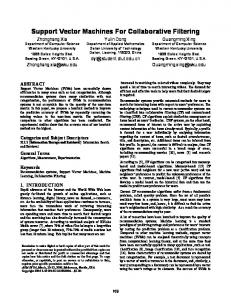
which is found to be superior to most existing object detection methods [11]. We first demonstrate an example in which the `observed' image is constructed by adding the `target' object to a background image and then adding white Gaussian noise. An image consisting of the values of the target kernel weights computed with the DFTRVM algorithm is shown in Fig. 1. Note that because of the RVM sparseness property, only few weights have non-zero values. The `target' object is the tank located at pixel (100, 50), where the bright white spot on the kernel weight image exists. When evaluating a detection algorithm it is important to consider the detection probability PD, which is the probability that an existing `target' is detected and the probability of false alarm PFA, which is the probability that a `target' is incorrectly detected. Any of these probabilities can be set to an arbitrary value by selecting an appropriate value for the threshold T. A receiver operating characteristics (ROC) curve is a plot of the probability of detection PD versus the probability of false alarm PFA, which provides a comprehensive way to demonstrate the performance of a detection algorithm. However, an ROC curve is not suitable for evaluating object detection algorithms because it only considers if an algorithm has detected an object or not; it does not consider if the object was detected in the correct location. Instead, we can use the localized ROC (LROC) curve, which is a plot of the probability of detection and correct localization PDL versus the probability of false alarm and considers also the location where a `target' has been detected. In order to evaluate the performance of the algorithm, we created 50 `observed' images by adding a `target' image to a random location of a background image, and another 50 `observed' images without the `target' object. White Gaussian noise was then added to each `observed' image. The DFT-RVM algorithm was then used to estimate the parameters of an RVM model with a `target' kernel and a Gaussian background kernel for each `observed' image, generating 100 kernel weight images. These kernel weight images were then thresholded for many different threshold values and estimates of the probabilities PDL and PFA were computed for each threshold value. Similar experiments were performed for the ARIR algorithm also. An LROC curve was then plotted for each algorithm, see Fig. 2. The area under the LROC curve, which is a common measure of the performance of a detection algorithm, is significantly larger for the DFT-RVM algorithm. It is important that the

LROC curve is high for small values of PFA, since usually the threshold is chosen so that only a small fraction of false detections are allowed [11].

Figure 2. LROC curves for the ARIR (left) and DFT-RVM (right) algorithms.

3.3. Applications on Computer-aided Diagnosis 3.3.1. Background Breast cancer is a common form of cancer diagnosed in women. One of the important early signs of breast cancer in mammograms is the appearance of microcalcification (MC) clusters, which appear in 30-50% of mammographically diagnosed cases [12]. MCs are calcium deposits of very small dimension and appear as a group of granular bright spots in a mammogram. As an example, Fig. 3 shows a mammogram image with a cluster of MCs. Individual MCs are sometimes difficult to detect because of the surrounding breast tissue, their variation in shape and small dimension. Because of its importance in breast cancer diagnosis, accurate detection and classification of MC clusters are very important problems.

(a)

(b)

Figure 3. (a) Mammogram in craniocaudal view. (b) Expanded view showing MCs.

3.3.2. Automatic detection of microcalcification clusters In recent years, there has been a great deal of research in development of computerized methods for automatic and accurate detection of MC clusters, which could potentially assist radiologists in diagnosis of breast cancer. A thorough review of various methods for MC detection reported in the literature can be found in [13]. In [14], we developed a support vector machine (SVM) approach for detection of clustered MCs in mammograms, and demonstrated that such an approach could outperform several well-known methods in the literature. While the SVM approach achieves the best detection performance, the computational complexity of the SVM classifier may prove to be burdensome in realtime or near real-time applications. In an SVM classifier, the decision function is determined by a subset of training samples (called support vectors); the computational complexity of the decision function is linearly proportional to the number of support vectors. As a consequence, too many a support vector can lead to a classifier (SVM) that is computationally expensive. This issue is especially important for MC detection, as modern digital mammography scanners can produce images at high resolutions, which may require significant computation time to process. To address this issue, in [15] we proposed to improve the computational efficiency of our previously developed SVM detection by using an alternative – relevance vector machine (RVM) – for MC detection. The advantage is that the RVM classifier can yield a decision function that is much sparser than the SVM while maintaining its detection accuracy. This can lead to significant reduction in the computational complexity of the decision function, thereby making it more suitable for real-time applications. Here MC detection is formulated as a binary classification problem. Specifically, at each location of a mammogram image, we apply an RVM classifier to determine whether an MC object is present or not. That is, for a given mammogram image, the MC detection process consists of the following two steps: 1) at each pixel location in the image, extract an input vector x to describe its surrounding image feature; 2) apply the RVM classifier f RVM (x) to decide whether x belongs to “MC present” class or “MC absent” class.

We define the input vector x to the RVM classifier to be formed by a small window of M × M pixels centered at the location of interest in a mammogram image. The choice of M should be large enough to cover an MC and yet small enough to avoid any interference from neighboring MCs. In the dataset used in this study, the mammograms were digitized at 0.05 mm/pixel, and M =15 was chosen empirically in our experiments. To suppress the background and thereby restrict the intra-class variations among the input samples, a high-pass filter with a narrow stop-band was applied to each mammogram image. The high-pass filter was designed to be a finite impulse response (FIR) filter with cutoff frequency wc=0.05 cycles/pixel and length 10. In summary, the input vector x is obtained at each pixel location as follows:

x = W [ Hf ] (42) where f denotes the entire mammogram image, H denotes the filtering operator, and W is the windowing operator. Note that for M = 15 , the dimension of x is 225. The training of the RVM classifier function consists of the following two steps: 1) collect training samples

{(xi , di ), i = 1, 2," , N }

from the existing

mammograms, 2) optimize the model parameters of the RVM classifier for best performance. To demonstrate the RVM classifier, we used a set of 141 mammograms from 66 clinical cases collected by the Department of Radiology at the University of Chicago. Each mammogram had one or more clusters of MCs which were histologically proven. These mammograms were digitized with a spatial resolution of 0.05 mm/pixel and 10-bit grayscale with a dimension of 3000 × 5000 pixels. The MCs in each mammogram were manually identified by a group of experienced radiologists. To save computation time, a section of 900 ×1000 pixels, containing all the identified MCs, was cropped from each mammogram such that it was free of nontissue areas. These section images were used in our subsequent experiments. In our study, we divided the dataset in a random fashion into two separate subsets, each containing 33 cases. Subsequently, mammograms in one subset were used for training the classifiers, and mammograms in the other subset were used exclusively for testing the classifiers. Thus, mammograms from the same case were used either for training or testing, but never for both.

The mammograms in the training subset were found to have a total of 1291 individual MCs. For each of these MCs, a window of M × M image pixels centered at its center was extracted; the vector formed by this window of pixels, denoted by xi , was then treated as an input pattern to the classifier for the “MC present” class ( d i = +1 ). This yielded a total of 1291 samples for the “MC present” class. Similarly, nearly twice as many (2232, to be exact) “MC absent” samples were collected ( d i = −1 ), except that their locations were selected randomly from the set of all “MC absent” locations in the training mammograms. In this procedure no sample window was allowed to overlap with any other sample window. For demonstration purpose, we show in Fig. 4 some examples of sample image windows for “MC present” and “MC absent” classes in the resulting training data set. To determine the fine-tuning parameters of the RVM classifier model for optimal performance, we apply a ten-fold cross validation in the training set. The best error level (4.89%) was obtained by an order-2 polynomial kernel. For the RVM classifier, the number of relevance vectors (produced during training) was found to be 65 (1.85% of the number of training samples). For comparison, we also trained an SVM classifier using the same data set. The number of support vectors was found to be 521 (14.79% of the number of training samples). Indeed, the RVM classifier is much sparser than the SVM. To gain further insight on the RVM classifier, we show in Fig. 5 the corresponding image windows for some relevance vectors from both “MC present” and “MC absent” classes; for comparison, we show in Fig. 6 the image windows for some support vectors of the SVM classifier. As can be seen, for the RVM the relevance vectors from the two classes are distinctly different. The “MC present” relevance vectors consist of MCs that are clearly visible, and the “MC absent” relevance vectors consist of image windows that do not show MC-like features at all. In a sense, the relevance vectors are formed by “easy-to-classify” samples from both classes. In contrast, for the SVM the support vectors from the two classes do not seem to be distinctly different, that is, the “MC present” support vectors could be mistaken for “MC absent” image regions, and vice versa. These support vectors are samples that appear to be “borderline”, “difficult-to-classify”. These results demonstrate that the two classifiers are quite different from each other.

“MC present” samples

15 ×15

Figure 4. Examples of

“MC absent” samples

image windows of training samples from the “MC present” and “MC absent” classes. These

are randomly selected from the training set.

“MC present” relevance vectors Figure 5. Examples of

15 × 15

“MC absent” relevance vectors

image windows of the relevance vectors (RVs) from the “MC present” and “MC absent”

classes. All the 19 “MC present” RVs are shown and only 25 of the 46 “MC absent” RVs are shown.

“MC present” support vectors Figure 6. Examples of

15 ×15

“MC absent” support vectors

image windows of the support vectors (SVs) from the “MC present” and “MC absent” classes.

The performance of the RVM classifier for detection of clustered MCs is summarized using free-response receiver operating characteristic (FROC) curves. An FROC curve [16] plots the correct detection rate (i.e. true positive fraction (TPF)) versus the average number of false-positives (FPs) per image varied over the continuum of the decision threshold. It provides a comprehensive summary of the trade-off between detection sensitivity and specificity. The trained classifiers were evaluated using all the mammograms in the test subset. The test results are summarized using FROC curves in Fig. 7. In particular, the RVM achieved a sensitivity of approximately 90% when the false positive rate is at one FP cluster on average per image. Interestingly, this sensitivity level is also similar to that achieved by the SVM. Compared to SVM, the RVM classifier has reduced the detection time from nearly 250 s to about 30 s per image, nearly an order of magnitude reduction. Experimental results showed that the RVM technique could greatly reduce the computational complexity of the SVM while maintaining its detection accuracy. This makes RVM more feasible for real-time processing of MC clusters in mammograms.

Figure 7. FROC curves of the different methods.

3.3.3. Classification of Microcalcification Clusters Once MCs are detected, another issue is how to classify them. Since these lesions appear in benign breast tissues as well as in malignant ones. They are often very difficult to diagnose accurately. It is reported that among those with radiographically suspicious, nonpalpable lesions who are sent for biopsy, only 15% to 34% are found to actually have malignancies [17][18]. There has been a great deal of research in recent years to develop computerized methods that potentially could assist radiologists differentiate benign from malignant MCs. In particular, Jiang et al [19] developed an automated computer scheme that was demonstrated to classify clustered

MCs more accurately than radiologists. This scheme made use of a feedforward artificial neural network (FFNN), which was trained to predict the likelihood of malignancy based on quantitative image features automatically extracted from the clustered MCs. It was subsequently demonstrated in [20] that when used as a diagnostic aid, this scheme could also lead to significant improvement in radiologists’ performance in distinguishing between malignant and benign clustered MCs. In [21] we investigated several state-of-the-art machine-learning methods including RVM, SVM, and Kernel Fisher’s discriminant for automated classification of clustered microcalcifications (MCs). In our study, classification of malignant from benign clustered MCs is treated as a two-class pattern classification problem, i.e., a microcalcification cluster (MCC) under consideration is either malignant or benign. The different classifier models were developed and tested using a data set collected by the Department of Radiology at the University of Chicago. This data set consisted of 697 mammograms from 386 clinical cases, of which all had lesions containing clustered microcalcifications which were histologically proven. Among them 75 were malignant, and the rest (311) were benign. Furthermore, most of these cases have two standard-view mammograms: mediolateral oblique (ML) and craniocaudal (CC) views. The clustered MCs were identified by a group of experienced researchers. For computer analysis, all the mammograms in the data set were digitized with a spatial resolution of 0.1 mm/pixel and 10-bit grayscale. The data set includes a wide spectrum of cases that are judged to be difficult to classify by radiologists. For automated classification, the following eight features [19][20], all computed from the mammogram images, were used to characterize an MCC: 1) the number of MCs in the cluster, 2) the mean effective volume (area times effective thickness) of individual MCs, 3) the area of the cluster, 4) the circularity of the cluster, 5) the relative standard deviation of the effective thickness, 6) the relative standard deviation of the effective volume, 7) the mean area of MCs, and 8) the second highest microcalcification-shape-irregularity measure. The numerical values of all these features were normalized to be within the range between 0 and 1. These features were selected to have intuitive meanings that correlate qualitatively to features used by radiologists [19]. This provides an important common ground for the computer scheme to achieve high classification performance and for radiologists to interpret the computer results.

For preparation of training and testing samples for the classifier models, the eight features are extracted for each MCC in the mammogram data set; the vector formed by the eight feature values, denoted by xi , is then treated as an input pattern, and is labeled as yi = +1 for a malignant case, and yi = −1 otherwise. Together,

( xi , yi ) forms an input-output pair. There are in total 697 such pairs obtained from the whole mammogram data set. These pairs are subsequently used for training and testing of the classifier models. To determine the fine-tuning parameters for each classifier model, we apply a leave-one-out cross validation procedure. To evaluate the performance of a classifier, we use the so-called receiver operating characteristic (ROC) analysis, which is now used routinely for many classification tasks. We list in Table I the estimate of Az and its standard deviation, obtained using the ROCKIT program [27], and the parametric settings resulted from the training procedure for the different classifier models. These results demonstrate that the kernel methods (RVM, SVM, and KFD) are similar in performance (in terms of Az ), significantly outperforming a well-established, clinically-proven CADx approach that is based on neural network. TABLE I. CLASSIFICATION RESULTS OBTAINED WITH DIFFERENT CLASSIFIER MODELS.

SVM

KFD

RVM

FFNN

Az

0. 8545

0.8303

0.8421

0.8007

Std. Dev.

0.0259

0.0254

0.0243

0.0266

Parameters

Order-2

Order-2

Order-2

3 layers,

polynomial

polynomial

polynomial

6 hidden

kernel,

kernel

kernel

neurons,

C=700

100 seeds

4. CONCLUSIONS The relevance vector machine (RVM) constitutes a powerful methodology for regression and classification tasks. It achieves very good generalization performance and yields sparse models that provide inference at moderate computational cost. However, during the training phase the inversion of a large matrix is required. This makes this methodology inappropriate for large datasets. This problem can be

partially overcome by a modified learning algorithm, based on building the desired model incrementally. For image data where a periodically sampled training set is available a methodology based on computations in the DFT domain has been described which can bypass these difficulties. Since RVM can be also used for classification tasks we present a successful example of RVM for microcalcification detection and classification. This example clearly demonstrates the advantages of RVM and illustrates its differences from SVM.

REFERENCES [1] V. Roth, “The Generalized LASSO”, Trans. on Neural Networks, vol 15, Jan 2004. [2] R. Tibshirani, “Regression shrinkage and selection via the LASSO”, J. Roy. Statist. Soc., vol. B 58, no. 1, pp. 267–288, 1996. [3] V. Vapnik, Statistical Learning Theory, New York: John Wiley, 1998. [4] Tipping M. E. “Sparse Bayesian Learning and the Relevance Vector Machine”, Journal of Machine Learning Research, pp. 211-244, 2001. [5] M. Figueiredo and A. Jain, “Bayesian learning of sparse classifiers,” in Proc. Computer Vision and Pattern Recognition, pp. 35–41, 2001. [6] Berger J.O. Statistical Decision Theory and Bayesian Analysis, 2nd Edition, Springer-Verlag, New York 1985. [7] C. Bishop, and M. Tipping, “Variational Relevance Vector Machines”, Proceedings of Uncertainty in Artificial Intelligence, 2000. [8] Tipping M. E., and Faul A. “Fast Marginal Likelihood Maximization for Sparse Bayesian Models” Proceedings of the Ninth International Workshop on Artificial Intelligence and Statistics, Jan 3-6, 2003 [9] J. L. Horner and P.D. Gianino, "Phase-only matched filtering", Applied Optics, 23(6), 812-816, 1984. [10] Q. Chen, M. Defrise and F. Decorninck, "Symmetric phase-only matched filtering of Fourier-Mellin transforms for image registration and recognition", Pattern Recognition and Machine Intelligence, 12(12), 1156-1198, 1994. [11] A. Abu-Naser, N. P. Galatsanos, M. N. Wernick and D. Shonfeld, “Object Recognition Based on Impulse Restoration Using the Expectation-Maximization

Algorithm”, Journal of the Optical Society of America, Vol. 15, No. 9, 23272340, September 1998. [12] Cancer Facts and Figures 1998. Atlanta, GA: American Cancer Society, 1998. [13] R. M. Nishikawa, “Detection of microcalcifications,” in Image-Processing Techniques for Tumor Detection, R. N. Strickland, ed, Marcel Dekker, Inc, New York, 2002. [14] I. El-Naqa, Y. Yang, M. N. Wernick, N. P. Galatsanos, and R. M. Nishikawa, “A support vector machine approach for detection of microcalcifications,” IEEE Trans. on Medical Imaging, vol. 21, 1552-1563, 2002. [15] L. Wei, Y. Yang, R. M. Nishikawa, M. N. Wernick and A. Edwards, “Relevance Vector Machine for Automatic Detection of Clustered Microcalcifications,” IEEE Trans. on Medical Imaging, vol. 24, 1278-1285, 2005. [16] P. C. Bunch, J. F. Hamilton, et al, “A free-response approach to the measurement and characterization of radiographic-observer performance”, J. Appl. Eng., vol. 4, 1978. [17] A. M. Knutzen and J. J. Gisvold, “Likelihood of malignant disease for various categories of mammographically detected, nonpalpable breast lesions,” Mayo Clin. Proc., vol. 68, pp. 454- 460, 1993. [18] D. B. Kopans, “The positive predictive value of mammography,” AJR, vol. 158, pp. 521-526, 1992. [19] Y. Jiang, R. M. Nishikawa, E. E. Wolverton, C. E. Metz, M. L. Giger, R. A. Schmidt, and C. J. Vyborny, “Malignant and benign clustered microcalcifications: Automated feature analysis and classification,” Radiology, vol. 198, pp. 671-678, 1996. [20] Y. Jiang, R. M. Nishikawa, R. A. Schmidt, C. E. Metz, M. L. Giger, and K. Doi, “Improving breast cancer diagnosis with computer-aided diagnosis,” Academic Radiology, vol. 6, pp. 22-33, 1999. [21] L. Wei, Y. Yang, R. M. Nishikawa, and Y. Jiang, “A study on several machinelearning methods for classification of malignant and benign clustered microcalcifications”, IEEE Trans on Medical Imaging, Vol. 24, No. 3, pp. 371380, March, 2005. [22] S. Chen, S. R. Gunn and C. J. Harris, “The relevance vector machine technique for channel equalization application,” IEEE Trans on Neural Networks, Vol. 12, No. 6, pp. 1529-1532, 2001.

[23] P. F. Yeung, H. S. Wong, B. Ma and H. H-S. Ip, “Relevance vector machine for content-based retrieval of 3D head models,” IEEE Intl. Conf. on Information Visualisation , pp. 425-429, July, 2005. [24] L. Carin and G. J. Dobeck, “Relevance vector machine feature selection and classification for underwater targets,” Proceedings of OCEANS 2003, Vol. 2, pp. 22-26, 2003. [25] D. G. Tzikas, A. Likas, N. P. Galatsanos, A. S. Lukic and M. N. Wernick, “Relevance vector machine analysis of functional neuroimages,” IEEE intel. Symposium on Biomedical Imaging, vol. 1, pp. 1004-1007, 2004. [26] D. Datcu and L. J. M. Rothkrantz, “Facial expression recognition with relevance vector machines,” IEEE intel. Conf. on Multimedia and Expo, pp. 193-196, 2005. [27] Metz CE, Herman BA, Roe CA. “Statistical comparison of two ROC curve estimates obtained from partially-paired datasets” Med Decis Making 18:110121, 1998.