CAREER grant IIS-0643298 and Chinese Scholarship Council. ... Engineering, Texas A&M University, College Station, TX 77843, United. States. ...... IEEE International Conference on Robotics and Automation, Orlando,. Florida, May 2006, pp.
A Two-View based Multilayer Feature Graph for Robot Navigation Haifeng Li, Dezhen Song, Yan Lu, and Jingtai Liu
Abstract— To facilitate scene understanding and robot navigation in a modern urban area, we design a multilayer feature graph (MFG) based on two views from an on-board camera. The nodes of an MFG are features such as scale invariant feature transformation (SIFT) feature points, line segments, lines, and planes while edges of the MFG represent different geometric relationships such as adjacency, parallelism, collinearity, and coplanarity. MFG also connects the features in two views and the corresponding 3D coordinate system. Building on SIFT feature points and line segments, MFG is constructed using feature fusion which incrementally, iteratively, and extensively verifies the aforementioned geometric relationships using random sample consensus (RANSAC) framework. Physical experiments show that MFG can be successfully constructed in urban area and the construction method is demonstrated to be very robust in identifying feature correspondence.
I. I NTRODUCTION When a mobile robot travels in a modern urban environment, the robot often needs visual signals from its onboard camera to assist navigation. A typical modern urban environment is usually rectilinear and consists of many structured objects and distinctive features such as vertical walls, parallel edges, orthogonal planes, etc. Extracting such features from video frames to form a quick scene understanding can directly benefit navigation tasks such as localization, mapping, obstacle avoidance, and motion planning. Here we design a multilayer feature graph (MFG) to facilitate the scene understanding in urban area. Nodes of an MFG are features such as scale invariant feature transformation (SIFT) feature points, line segments, lines, and planes while edges of the MFG represent different geometric relationships such as adjacency, parallelism, collinearity, and coplanarity. MFG also connects the features in two views and the corresponding 3D world coordinate system. Fig. 1 illustrates the MFG in the 3D world coordinate system. We design an MFG construction method using a feature fusion process which incrementally, iteratively, and extensively verifies the aforementioned geometric relationships using random sample consensus (RANSAC) framework. We have implemented MFG construction algorithm and tested it in physical experiments. Results show that MFG can be successfully constructed from raw image data. Since the process utilizes multiple types of geometric relationships, This work was supported in part by National Science Foundation under CAREER grant IIS-0643298 and Chinese Scholarship Council. H. Li and J. Liu are with the Institute of Robotics and Automatic Information System, Nankai University, Tianjin 300071, P. R. China. Emails: {lihf, liujt}@robot.nankai.edu.cn. D. Song and Y. Lu are with the Department of Computer Science and Engineering, Texas A&M University, College Station, TX 77843, United States. Emails: {ylu, dzsong}@cse.tamu.edu.
vv
1
2
l1
l2
p2
p1
v1
v2 3
1
2
Fig. 1. An illustration of the multilayer feature graph. Based on vanishing points, building facades, parallel line/line segment groups, and feature points, an MFG is a feature-based scene reconstruction which focuses on robot navigation needs. The camera frame at the top left corner is one of the input two views and the output is the MFG.
the feature correspondence outcome is significantly improved over existing feature matching methods. As an important part of MFG, the algorithm is able to detect all primary vertical planes with reasonable accuracy. II. R ELATED W ORK Our MFG is a novel scene understanding and knowledge representation method for vision-based robot navigation in urban area. A mobile robot usually has different ways of constructing and representing its surrounding environments, which usually depend on different sensors, 3D reconstruction schemes, and feature matching methods. The most common sensors for robot navigation include sonar arrays [1], laser range finders [2], [3], depth cameras [4], regular cameras [5]–[9], or their combinations [10], [11]. Simultaneous localization and mapping (SLAM) is the typical framework employed by robot navigation [12] to make decisions based on the sensory input. In a SLAM framework, the physical world is represented as a collection of “landmarks.” For example, landmarks are point clouds if a laser ranger finder or a depth camera is the primary sensor. In vision-based SLAM, SIFT feature points or its variants [5], [6], [13] and line features [7]–[9] are often employed as landmarks. Landmarks can be viewed as a rudimentary way of scene understanding which serves SLAM purposes well. Our MFG complements SLAM approaches because a better scene understanding method can also increase the robustness of localization results and make it easy to utilize prior knowledge such as existing maps. In computer vision and graphics field, 3D reconstruction
has been a very popular topic for research as well as commercial applications. Sensors used there also include laser range finder [14] and more often, aerial cameras [15]. Google Earth and Microsoft Virtual Earth are successful showcases for 3D reconstruction of city models [16]. Following the taxonomy of Seitz et al. [17], 3D reconstruction algorithms can be categorized into four classes: voxel approaches [18], level-set techniques [19], [20], line segment matching [21], polygon mesh methods [22], and algorithms that compute and merge depth maps [23], [24]. Unlike those methods, our MFG does not pursuit a full scale reconstruction and hence does not require intensive computation or suffers from occlusion, correspondence, and lighting problems in the field. Our MFG focuses on key features that represent building facades and orthogonal/parallel lines which are insensitive to illumination and shadow problems caused by natural lighting. In a closely related work, Cham et al. [25] identify vertical corner edges of buildings as well as the neighboring plane normals from a single ground-view omnidirectional image to estimate the camera pose. Recent work by Delmerico et al. [26] proposes a method to determine a set of candidate planes by sampling and clustering points from stereo images with RANSAC using estimated local normals. These methods provide the inspiration that planes are important and robust features to be extracted in reconstruction. However, our MFG does not rely on the depth information from existing stereo images or a specialized imaging device. MFG simply employs multiple types of features and utilizes multiple internal geometric relationships between features for better robustness and applicability. Properly matching multiple types of features across views is essential to MFG construction. Although point feature matching [13], [27] is relatively mature, line segment matching is very challenging due to inaccurate end points, occlusion, and complex correspondence. Schmid and Zisserman [28] utilize the epipolar constraints of line segment end points for matching, which requires the prior knowledge of epipolar geometry. The color-based methods [29]–[31] perform poorly when color features are not distinctive and hence are sensitive to illumination conditions. Other grouping matching methods [32], [33] are limited by either high computational complexity or sensitivity to inaccurate endpoints of line segments. Recently, Fan et al. [34] propose a line segment matching method by leveraging feature point correspondences in adjacent regions. This is the best available method for line segment matching and is named as “point-based line matching (PBLM)” in this paper. This method is promising but still misses many line segment matches due to lack of feature points. Inspired by this method, our MFG addresses these issues by introducing ideal lines and analyzing collinear and coplanarity relationships. Our group has worked on robot navigation using passive vision system in past decade. We have developed appearancebased method [35], investigated how depth error affects navigation [36], and used vertical line segments for visual odometry tasks [37], [38]. In the process, we have realized it is necessary to combine benefits of different features to
assist navigation which leads to this work. III. P ROBLEM D EFINITION A. Assumptions To formulate the problem and focus on the most relevant issues, we have the following assumptions. • • •
•
The robot is in a modern urban environment where rectilinear polygonal buildings dominate the scene. To assist scene understanding, the robot is equipped with a gravity sensor and knows its vertical direction. The intrinsic parameters of the finite perspective camera are known by pre-calibration. The lens distortion of the camera has been removed. The robot knows baseline distance for two views. This can be achieved with on-board inertial sensors or wheel encoders. These sensors are good at short distance measurement. It is worth noting that the measurement may contain error. We use the measurement as an initial input and the baseline distance will be refined during the image feature maturing process.
B. Notations, Coordinate Systems, and Problem Definition In this paper, all the coordinate systems are right hand systems. The superscript ′ denotes the corresponding notation in the second view. Notations in the format of (a, a′ ) refer to a corresponding pair of variables or parameters in the first and second views, respectively. Let us define • •
•
• •
{W } as a 3D Euclidean world coordinate system (WCS) with its x − z plane being horizontal, {C} and {C′ } as two 3D camera coordinate systems (CCS) for the first and the second views, respectively, (For each CCS, its origin is at the camera optical center, its z−axis coincides with the optical axis and points to the forward direction of the camera, its x−axis and y−axis are parallel to the horizontal and vertical directions of the CCD sensor plane, respectively.) {I} and {I ′ } as two 2D image coordinate systems (ICS) for the first and the second views, respectively, (For each ICS, its u−axis and v−axis are parallel to x and y axes of the corresponding CCS, respectively) Fr and Fr′ as the raw images taken at the first and the second views, respectively, and K as the intrinsic parameter matrix of the camera.
With these notations defined, our problem is, Definition 1: Given Fr and Fr′ , construct the MFG. Now let us introduce MFG. IV. M ULTILAYER F EATURE G RAPH Fig. 2 illustrates how MFG organizes different types of features according to their geometric relationships. The bottom layers of MFG are raw features such as SIFT points and line segments while the top layers of MFG contain planes describing the structure of the scene. To explain the structure of MFG, we begin with the raw feature extraction.
vanishing points
v2
v1
vv
parallelism
vertical planes
i
1
q
coplanarity ideal lines
la
lb
ld
lc
collinearity line segments
c
b
a
d adjacency
SIFT points
pa Fig. 2.
pb
pc
pd
The structure of the multilayer feature graph.
is the normal vector of πi , and di is the distance from the camera center to πi . Note that we do not include horizontal planes in the design because horizontal planes represent either road planes or building top planes. The former does not exist when road is not flat and the latter is not visible from a ground robot. If an ideal line is located in a vertical plane, an edge between the two nodes is established in MFG. A vertical plane must have at least two child nodes because two lines determine a plane when they are either intersecting or being parallel to each other. An ideal line may not necessarily have a parent node if it corresponds to an isolated linear object such as a light pole. An ideal line may have two parent vertical planes if it is a boundary line. D. Layer 5: Vanishing Points
A. Layers 1&2: Raw Features SIFT points and line segments are the raw features of MFG (see Fig. 2). Define P := {p1 , p2 , . . .} as the SIFT point feature set with pi being the i-th SIFT point feature. Line segments are extracted using the line segment detector (LSD) method [39]. Define ιi = [Ei,0 , Ei,1 ]T as the i-th line segment with its two end points: Ei,0 = [ui,0 , vi,0 ]T and Ei,1 = [ui,1 , vi,1 ]T . Let L = {ι1 , ι2 , . . . , ιn } denote a line segment set with each element being a line segment in ICS. Each SIFT point or line segment represents a node in MFG. If a SIFT point is in the neighborhood (will be defined later in the paper) of a line segment, then an edge between them is established with the line segment being the parent node. It is possible that a line segment node does not have any child SIFT nodes (ιd in Fig. 2). A SIFT node may have multiple parent line segment nodes (pb in Fig. 2). Note that SIFT points are only used to assist line segment matching in the paper. That is why we exam their adjacency to line segments. B. Layer 3: Ideal Lines To aggregate line segments and extract potential lines from the raw features, we introduce ideal lines. Definition 2: An ideal line is defined as a real or virtual line passing through a set of collinear line segments. An ideal line might/might not correspond to a real line in 3D space. Define L = {l1 , l2 , . . . , lm } as an ideal line set with li , i = 1, . . . m, being an ideal line in ICS. For a given set of collinear line segments {ιa , ιb , . . .}, its ideal line li is obtained by fitting the line through the end points of all line segments in the set using the maximum likelihood estimation (MLE) method [40]. As shown in Fig. 2, each line segment must have only one corresponding ideal line as its parent node. An ideal line may have multiple child line segment nodes. An ideal line usually has three representations: 3D format in {W } and two 2D formats in {I} and {I ′ } of the two views, respectively. C. Layer 4: Vertical Planes Vertical planes in {W } form layer 4. Let πi , i = 1, 2, . . . , q, denote vertical planes in {W } and πi = [ni , di ]T , where ni
In a vertical plane, there usually are many parallel ideal lines. Those parallel ideal lines intersect each other at vanishing points. Each vertical plane usually has two groups of parallel ideal lines: one horizontal group and one vertical group from building and window boundaries. Therefore, each vertical plane has two dominating vanishing points. Fig. 2 illustrates the relationship by connecting each vertical plane node to two parent vanishing point nodes. Since modern urban area is largely a rectilinear environment, there usually are three dominating vanishing points with one being vertical (denoted as vv ) and two being horizontal (denoted as v1 and v2 ). For simplicity, we use three vanishing points in the rest of the paper although the approach can be adaptive to varying numbers. Fig. 2 also shows that a vanishing point may correspond to parallel ideal line groups in different planes. For example, the vertical vanishing point node links to every vertical plane node with vertical ideal lines. V. MFG C ONSTRUCTION VIA F EATURE F USION Constructing MFG is nontrivial. It is a scene understanding process. Raw features in layers 1&2 and vanishing points in layer 5 are straightforward to obtain using existing methods. However, ideal lines and vertical planes, which represent structure of the scene at different granularity, are difficult to compute because proper correspondence between two views needs to be established. Fig. 3 illustrates the process of MFG construction, which is named as feature fusion. The process can be divided into three main components: parallelism, collinearity, and coplanarity verifications. A. Parallelism Verification The purpose of parallelism verification is to divide line segments and ideal lines into different parallel groups and find group correspondence across the two views. Since parallel lines intersect each other at vanishing points, vanishing points are natural classifiers for the parallelism verification. Steps 1-5 in Fig. 3 illustrate the procedure. In step 1, raw line segments are extracted using LSD. We then apply RANSAC framework to line segments to estimate vanishing points. Since we know the vertical direction from gravity
Points 0(a). Compute SIFT points
Line segments
Ideal lines
1. Line segments extraction
2. Vanishing point estimation
F 0(b). Putative SIFT point matching
L, L
3. Perspective correction
4. Ideal line generation
L, L'
5. Vanishing point matching
(P, P ' )
6. Initial line segment matching
Parallelism Verification
Collinearity Verification
9(b). Vertical line segment refinement
9(a). Plane estimation and guided matching for vertical ideal lines
10(b).Horizontal line segment refinement
10(a). Plane estimation and guided matching for horizontal ideal lines
a
MFG
vv
la 1
b
pb
v1
lb i
A block diagram for multilayer feature fusion.
sensors, it is easy to identify vanishing point vv which corresponds to vertical line segments. It is worth noting that vv must exist because urban buildings have many vertical boundaries. Horizontal vanishing points can be found by the following orthogonality check, ∥vv T ω vˆ i ∥ < ε ,
establish scene understanding. In fact, we need to establish cross view correspondence between line segments and ideal lines. However, one-to-one correspondence for line segments is impossible to achieve due to severe occlusion and noises. Collinearity verification is proposed to handle the challenge. B. Collinearity Verification
Coplanarity Verification
pa
Fig. 4. An example of vanishing point matching across F and F ′ . The line segments and ideal lines associated with the same vanishing points are drawn in the same color (black, blue and red). In this example, vertical lines appear vertical because F and F ′ are results of the perspective correction.
7. Initial ideal line matching
8. Ideal line-guided line segment matching
Fig. 3.
F'
'
Collinearity verification is to find the correspondences of ideal lines and hence line segments across two views. This process also establishes ideal lines and line segments in {W }. A corresponding pair of line segments or ideal lines must be in the same parallel groups defined by the same vanishing points, which can help us reduce the matching problem size. Since a corresponding pair of line segments in the two views do not necessarily have corresponding end points due to occlusion and camera perspective issues, checking end point correspondence is not viable. Also an one-to-one correspondence does not necessarily exist. In fact, many-toone and one-to-many mappings are not unusual. Collinearity verification is designed to handle these challenging issues. Steps 6-8 in Fig. 3 illustrate the process. We first find the initial candidate correspondences for line segments using the PBLM method [34] (step 6). For completeness, we brief the PBLM method using Fig. 5.
(1)
where vˆ i is a candidate horizontal vanishing point, ω = (KKT )−1 is the image of the absolute conic, and ε is a small positive threshold. After identifying vanishing points, we can perform the perspective correction [40] for both views to make v-axes of ICSs to be vertical and therefore all vertical lines appear vertical in the two views (step 3). We define F and F ′ as the first and second views after the perspective correction, respectively. Meanwhile, initial set of ideal lines in {I} and {I ′ } can be established using MLE and RANSAC as well (step 4). Ideal lines can be associated with line segments in each view based on the inlier set of the RANSAC output. With the three vanishing points, the ideal lines and line segments in each view can be classified into three groups. This allows us to match different parallel groups across two views by matching vanishing points [41] (step 5). Fig. 4 illustrates the result of the vanishing point matching. The correspondence between two views for parallel groups by vanishing point matching is still too gross to be used to
F
F'
Fig. 5. An example of initial line segment matching using PBLM in [34].
For line segment ι j , we define its neighbor region as Ne(ι j ). The doted rectangles in Fig. 5 are the neighbor regions. ι j bisects Ne(ι j ) which has a half side length of dt along the direction perpendicular to ι j . On the other hand, we apply SIFT to F and F ′ . If a SIFT point pi lies in the neighbor region, then we denote it as pi ∈ Ne(ι j ). The initial line segment matching uses putative SIFT point correspondences: for each putative point pair (pi , p′i ), if pi ∈ Ne(ιa ) and p′i ∈ Ne(ιb′ ), then the similarity between ιa and ιb′ increases by 1. The initial line segment matches are determined by thresholding the overall similarity. The pro of this method is that it does not depend on end point matching while the con is that it may miss many
potential matches due to lack of features. We need to refine the results using ideal lines. Steps 7 and 8 in Fig. 3 show the process. Using initial line segment correspondences, we can tentatively match the ideal lines: given two ideal lines lm and ln′ in two views, we can determine lm and ln′ as a corresponding pair if the following is true, ∃ιi ∈ lm , ι ′j
∈ ln′
(ιi , ι ′j ) ∈ Sι ,ι ′ ,
s.t.
l1
2
1
F Fig. 6.
' 1
l
' 1
a
4 a
d
b
8
2
6
4
b
7 3
d
c
c
1
6
1
7
3
5
5
F'
F (a) Vertical Features
(2)
where Sι ,ι ′ is the set of all initial line segment matches. In step 8, we use the matched ideal line pairs to search for more line segment matches missed by the initial matching in step 7. Fig. 6 shows an example, where (l1 , l1′ ) is a pair of corresponding ideal lines obtained from the matched line segment pair (ι1 , ι1′ ). (ι2 , ι2′ ) was not matched in the initial matching step due to lack of SIFT features in the neighbor region. There is no correspondence for ι3 in the second view due to occlusions. Applying MSLD [31] metric, the line segment correspondence (ι2 , ι2′ ) is found. Furthermore, (l1 , l1′ ) helps us find the many-to-many correspondence [(ι1 , ι2 , ι3 ), (ι1′ , ι2′ )] across two views. Note that not all line segment or ideal line correspondences are correct at this step. However, most wrong matches can be removed by checking coplanar relationship next.
3
8
2
' 2
F'
An example of ideal line-guided line segment matching.
8
3 4
b
8
3 4
d
7
d
5
c
b 6
6 1
a
1 5
a
c
2
2
F
F'
(b) Horizontal Features Fig. 7. Coplanarity verification. These ideal line and line segments are classified into two groups representing in different colors (black and red) according to their residing vertical planes.
K, R2×2 is the 2D rotation matrix, and t2×1 = [tx ,tz ]T denotes the translation between the two camera centers. According to [40], line πi = [nT2×1 , d]T introduces a 1D homography for corresponding points in the two views, H2×2 = K2×2 (R2×2 − t2×1 nT2×1 /d)K−1 2×2 ,
(3)
where R2×2 can be computed from one pair of horizontal vanishing point correspondence, t2×1 is measured by onboard sensors, and n2×1 is a unitary vector. Only n2×1 and d are the unknown variables to be estimated. H2×2 has 2 degrees of freedom. Let ui and u′i be the u−coordinates of vertical ideal lines li and li′ , respectively. Denote ui = [ui , 1]T and u′i = [u′i , 1]T as the homogeneous coordinates. From the definition of homography, we know u′i = H2×2 ui .
C. Coplanarity Verification So far, we have completed the construction of layers 1, 2, 3, and 5 of MFG. The remaining layer 4 consists of vertical planes, which represent building facades and are of great importance for robot navigation. Layer 4 only exists in {W }. Coplanarity verification is designed to classify the coplanar features and reconstruct these planes. The coplanar verification process associates ideal lines to their residing planes (i.e. forming edges between ideal lines and vertical planes in MFG in Fig. 2). The process also removes false correspondences and finds more correspondences missed by previous steps. 1) Coplanarity Verification for Vertical Features: This process is done in two stages. Step 9(a) in Fig. 3 refers to the first stage where we estimate vertical planes from vertical ideal lines and use the plane to verify vertical line matches. In a top-down view, a vertical plane is reduced to a single line πi = [nT2×1 , d]T on the x − z plane of {W }. All the vertical ideal lines are reduced to points on the plane. Also, the 2D camera degenerates into a 1D camera. For the two 1D views, we define the camera matrices as P2×3 = K2×2 [I2×2 |02×1 ] and P′2×3 = K2×2 [R2×2 |t2×1 ], respectively, where the intrinsic parameters of the 1D camera, K2×2 , can be easily determined from the 2D camera parameter matrix
7
(4)
Define Ha,b as the (a,b)-th entry of H2×2 . Opening (4) and combining the resulting two equations, we have ui H1,1 + H1,2 − ui u′i H2,1 − u′i H2,2 = 0.
(5)
Eq. (5) has two unknown variables. Given 2 pairs of coplanar vertical ideal lines, we can compute the minimal solution of H2×2 by solving the two equations. All coplanar vertical ideal lines can be found using RANSAC iteratively, which selects a subset of inliers to minimize the geometric error, ′ ′ ˆ (6) ∑ dg (ui , Hˆ −1 2×2 ui ) + dg (ui , H2×2 ui ), i
ˆ 2×2 is where dg (·) denotes the geometric distance and H ˆ 2×2 is used to verify the cross the estimation of H2×2 . H view vertical ideal line correspondences. It is clear that a correctly corresponded ideal line pair must satisfy the homography. Hence we can refine the cross view vertical ideal line correspondences by removing false correspondences and searching for new correspondences to increase vertical ideal ˆ 2×2 and line inlier set for each plane. The estimation of H the refinement process can be iterated until the cross view vertical ideal line correspondences are stable.
Correspondingly, the change of cross view vertical ideal line correspondence in the refinement process changes line segment correspondences in the lower layer. We refine vertical line segment correspondences, which is the second stage (step 9(b) in Fig. 3). Fig. 7(a) illustrates the sample output of this process. ˆ 2×2 also allows us to compute vertical plane in the topH down view. Define B = K−1 2×2 H2×2 K2×2 . According to (3), we can obtain d and n2×1 as follows, d=√
1 B R −B2,1 R1,1 2 B1,2 R2,2 −B2,2 R1,2 2 ( 1,1B1,12,1tz −B2,1 tx ) + ( B1,2 tz −B2,2 tx )
d(B1,1 R2,1 −B2,1 R1,1 ) B tz −B2,1 tx n2×1 = d(B1,21,1 R2,2 −B2,2 R1,2 ) , B1,2 tz −B2,2 tx
,
VI. E XPERIMENTS (7)
where Ba,b and Ra,b are the (a,b)-th entry of B and R2×2 , respectively. 2) Coplanarity Verification for Horizontal Features: Candidate vertical planes found in the previous step can be further refined using horizontal line features (see Fig. 7(b)). Horizontal line features can help remove false positive planes and improve accuracy of vertical planes. Furthermore, we can remove falsely matched horizontal features and group the inliers based on the vertical planes (step 10 in Fig. 3). A pair of corresponding lines (li , li′ ) in two views can be related by a 2D homography li = HT3×3 li′ . According to [40], the 2D homograph can be obtained as follows, H3×3 = K(R3×3 − t3×1 nT3×1 /d)K−1 ,
We have implemented our MFG construction algorithm using Matlab 2008b on a laptop PC with an Intel 2.26Ghz Core 2 Duo CPU, 3GB RAM, a 160GB hard disk and a Windows XP OS. In the physical experiments, we use a BenQ DCE1035 camera with a resolution of 640 × 480 pixels. For the testing dataset, we have taken 8 different pairs of image on Texas A&M campus. For each pair, the baseline distance between two views is 5.5 m. The orientation settings of the camera are set to ensure a good overlap between the two views. Fig. 8 illustrates the first view of the 8 pairs. The algorithm has not been optimized yet. The average time for constructing an MFG from one image pair is 42 sec.
1
2
3
4
5
6
7
8
(8)
where R3×3 denotes the 3D camera rotation, t3×1 = [tx ,ty ,tz ]T is the translation between camera center positions of the two views, and n3×1 = [nx , ny , nz ] is the normal vector of the plane. ny = 0 because the plane is vertical. Comparing H2×2 in (3) and H3×3 in (8), we find that R3×3 and n3×1 can be directly obtained from R2×2 and n2×1 , respectively. tx /d and tz /d are both known from H2×2 . Given H2×2 , there is only one degree-of-freedom left in H3×3 . Therefore, the minimal solution of H3×3 can be computed using one horizontal line correspondence and the ˜ 2×2 = resulting H2×2 from the previous step. Defining H −1 −1 ˜ K2×2 H2×2 K2×2 , H3×3 = K H3×3 K, we have H˜ 1,1 0 H˜ 1,2 ˜ 3×3 = −nxty /d 1 −nzty /d , H (9) H˜ 2,1 0 H˜ 2,2 ˜ 2×2 . In H ˜ 3×3 , the only where H˜ a,b is the (a, b)-th entry of H unknown is ty . Note that we use a˜ indicate variable a is in normalized coordinates in this paper. Define l˜i = KT li and l˜i′ = KT li′ where (li , li′ ) is a corresponding pair of horizontal ideal lines. Denote l˜i = [a1 , a2 , a3 ]T and l˜i′ = [a′1 , a′2 , a′3 ]T as the homogeneous coordinates of l˜ and l˜′ , respectively. Pair (l˜i , l˜i′ ) satisfies 2D ˜ T l˜i′ . Thus homography by l˜i = H 3×3 a2 a′1 H˜ 1,2 − a2 a′2 nzty /d + a2 a′3 H˜ 2,2 = a3 a′2 .
Combining (9) and (10), we can obtain the minimal solution of H3×3 . The coplanar horizontal lines can be found using RANSAC iteratively. The homography-guided refinement of correspondences for horizontal ideal lines and line segments are similar to the process for vertical features. Following the principle of the Gold Standard Algorithm approach in computer vision [40], the final inlier set of coplanar vertical and horizontal lines are used to re-estimate πi ’s using MLE to improve accuracy. With πi ’s obtained, this completes the construction of MFG.
(10)
Fig. 8.
Sample images of the dataset.
A. A Sample Output Our algorithm has successfully constructed MFG. As a sample output, Fig. 9 illustrates the intermediate output of correctly matched line segments for the 8-th pair in Fig. 8. Four vertical planes have been identified in the figure.
1 23 38 32 2 34 22 19 22 34 27 1 28 40 4 1425 7 33 35 45 19 42 3951 2629 13 1549 3 36 7 529 1146 48 47 84 50 44 83017 31 26 16 16 5 24 24 4
5 8 21 9 32 1 6 76
7 20
17
1 9 5238 46 468 47 829 71 30 3949 33 828 74 6 12 66 30 32241 33 657614 75 37 67 77 79 5341 26 3 37 4717 94 37 43 34 16 3 381 42 48 13 25 15 24 27 5 9 52 10 1211 14 6059 32 44 2 22 12 10 55 434 7 1950 20 218 45 2527 24 20 55 6 85 31 50 99 82 6359 1169 36 6 5 35 36 93 35 1018 5348 64 22 20 15 86 26 523046 108 105 5831 6 36 89 98 4934 90 72 3384 13 18 80 91 83 81 92 87 70 96 102 21 2123 37 18352318 88 10656 95 51 11 7 40 73 97 62 3121 43 40 100 144315 6041 6239529 61 424538 3 21101 2717 51 54 10 5716 58 54 6 9 9 5619 28 107 103 25 53 104 15 12 32 63 61 13 57 9 8 2844 23 78
1
15
62 37 8 11 21 1014 4 22 1 12 2 4 20 9
8
7 1 20 23 5 21 19 22 32 4 1 6 33 4542 6 35 7 13 3 84
313 5 16 17 10
50
44 5 24
19 4
37 469 39 33468 4729 22 3830 8 34 8 286 34 71 74 2740 30 38 12 66 657614 75 37 32 43 3 37 241 9453 41 33 2667 77 15 4328 47 17 32 5249 14257 79 316 1 38 48 2 4213 25 5 32 22 2 52 1211 14 1 27 6059 24 44 12 19 50 29 51 10 7 10 4 34 39 10 919 63 25 20 55 45 5911 9 85 64 218 55 2635 24 20 27 31 50 6 6999 82 3693 6 35 5348 22 5230 46 5 36 86 26 20 15 1549 105 583389 90 108 6 31 49 34 80 36 72 91 18 84 36 7 46 13 18 8398 102 81 52947 11 48 87 70 96 92 21 2123 37 106 56 18 352318 88 95 83017 517 40 26 3116 73 11 16 24 40 62 3121 43 100 15 97 1443 623929 604538 41 42 61 54 5 3 21101 271751 10 107 5716 54 6 9 9 5619 2858 15 103 25 53 12 32 63 61 1378 57 9 104 8 28 44 23 17 10
15
62 37 8 11 21 1014 4 1 22 12 2 4 920 19 5 3 13 16 17
7 8 8
7
Fig. 9. Sample output for the MFG construction. We use the same color (blue yellow, red, and green) for correctly matched line segments in the same residing vertical plane.
Testing the functionality is just the first step of experiments. Two more experiments have been conducted to verify MFG. The first experiment is to verify its robustness by checking if MFG can find better correspondence between
line segment features. This is important because the rest of MFG depends on the correspondence accuracy. B. Robustness of Line Segment Matching One key advantage of MFG is that it verifies line segments using multiple types of geometric relationships. If successful, the line segment correspondence is supposed to be more robust than the existing line segment matching method. Since the best available method for line segment matching is the PBLM in [34] and the MFG construction algorithm has adopted the approach to find initial correspondence in Section V-B, the comparison essentially tries to find if our parallelism, collinearity, and coplanarity verifications can improve the matching results. The threshold of SIFT point matching in PBLM is set to 0.85. We compared the number of total matches (TM) and correct ratios (CR) between the two methods. Table I shows the matching performance using the aforementioned dataset. The last two columns of the table refer to how much TM and CR of MFG are more than those of PBLM, respectively. It can be seen that MFG can identify significantly more correctly matched line segments than those of PBLM. Also, CRs of MFG are larger than those of PBLM for all cases except the second pair. TABLE I L INE SEGMENT MATCHING RESULTS : PBLM No. 1 2 3 4 5 6 7 8
PBLM TM CR 224 93.3% 157 94.9% 124 92.7% 186 93.5% 157 93.0% 219 93.6% 126 94.4% 194 92.3%
TM 297 289 178 282 274 302 189 314
MFG CR 95.6% 92.0% 96.2% 96.1% 95.3% 94.0% 94.7% 95.5%
VS .
MFG.
TM difference 73 132 54 96 117 83 73 120
CR difference 2.3% -2.9% 3.5% 2.6% 2.3% 0.4% 0.3% 3.2%
C. Vertical Plane Detection and Reconstruction Our second experiment is to verify if the MFG construction algorithm can properly identify vertical planes and to exam the accuracy of vertical plane reconstruction. Denote πˆi and π¯i as the estimation from the MFG construction and the ground truth of vertical plane πi , respectively. Ground truth π¯i is obtained by using three non-collinear 3D points lying in πi . The coordinates of the 3D points are obtained using a BOSCH GLR225 laser distance measurer with a range up to 70 m and measurement accuracy of ±1.5mm. Baseline distances are measured with a tape measure. Directly comparing πˆi to π¯i is not meaningful because the result depends on coordinate system and unit selections. To avoid the problem, we utilize the 3D point reconstruction error in comparison. Define x j as a 2D image point lying in πi . With the aid of camera intrinsic parameters and plane equations, we can reconstruct this point from π¯i and πˆi , respectively. Let X¯ j and Xˆ j be the corresponding results. We ∥X¯ −Xˆ ∥
define a relative error metric as ∥jX¯ ∥ j where ∥·∥ represents j the Euclidean distance. For each vertical plane, we manually
select 20 image feature points as even as possible to cover the whole plane region in the image. The mean value and standard deviation of the relative errors are shown in Table II for the dataset. TABLE II P ERCENTILE RELATIVE ERRORS OF THE RECONSTRUCTED 3D
π1 No. 1 2 3 4 5 6 7 8
mean 2.58 3.33 4.02 4.10 3.43 5.18 4.08 4.88
π2 std. dev. 0.82 0.48 1.28 1.03 0.14 0.74 0.16 0.29
mean 4.11 3.16 4.49 4.67 4.43 4.02 4.18 3.00
π3 std. dev. 1.18 0.88 0.92 0.41 0.28 0.64 0.43 0.48
POINTS .
π4
mean
std. dev.
4.37 2.64 5.20 4.41
0.28 0.44 0.47 0.15
mean
std. dev.
6.01
0.26
Tab. II shows that the algorithm has the ability to identify vertical planes in the images, which results in the different numbers of vertical planes for the image pairs in the dataset. The relative errors of points on planes are reasonably small which indicates that the estimate planes are reasonably accurate. The MFG construction algorithm design is successful. VII. C ONCLUSION AND F UTURE W ORK We reported a multilayer feature graph (MFG) to facilitate the robot scene understanding in urban areas. Nodes of an MFG were features such as SIFT feature points, line segments, lines, and planes while edges of the MFG represented different geometric relationships such as adjacency, parallelism, collinearity, and coplanarity. MFG also connected the features in two views and the corresponding 3D coordinate system. Our MFG construction method was a feature fusion process which incrementally, iteratively, and extensively verified the aforementioned geometric relationships using the RANSAC framework. We implemented the MFG construction method and tested it in physical experiments. Results showed that MFG can be successfully established and the feature correspondence outcomes were significantly improved over existing feature matching methods. The current result is just an initial step for MFG. In the future, we plan to address the N-View (N > 2) construction of MFG by combining bundle adjustment idea with error analysis into MFG. We will analyze computation complexity and develop efficient data structures for MFG. We will also investigate how to evolve MFG into an incremental update process so that it can be efficiently constructed for continuous image streams from mobile robots. Distributed and parallel implementation of MFG will be another direction to be explored. Applying MFG to GPS-less robot localization will be an immediate application if Google street view database is used. We will present these developments in future publications. ACKNOWLEDGMENT Thanks for C. Kim, W. Li, and H. Ge for their inputs and contributions to the Networked Robots Laboratory in Texas A&M University.
R EFERENCES [1] A. Elfes, “Sonar-based real-world mapping and navigation,” Robotics and Automation, IEEE Journal of, vol. 3, no. 3, pp. 249 –265, june 1987. [2] A. Diosi and L. Kleeman, “Laser scan matching in polar coordinates with application to slam,” in Intelligent Robots and Systems, 2005.(IROS 2005). IEEE/RSJ International Conference on. Alberta, Canada: IEEE, Aug. 2005, pp. 3317–3322. [3] V. Nguyen, A. Harati, A. Martinelli, R. Siegwart, and N. Tomatis, “Orthogonal slam: a step toward lightweight indoor autonomous navigation,” in Intelligent Robots and Systems, 2006 IEEE/RSJ International Conference on. Beijing, China: IEEE, Oct. 2006, pp. 5007–5012. [4] P. Henry, M. Krainin, E. Herbst, X. Ren, and D. Fox, “Rgb-d mapping: Using depth cameras for dense 3d modeling of indoor environments,” in the 12th International Symposium on Experimental Robotics, New Delhi & Agra, India, Dec. 2010. [5] E. Eade and T. Drummond, “Scalable monocular slam,” in IEEE Conference on Computer Vision and Pattern Recognition (CVPR) 2006, vol. 1. New York, NY, USA: IEEE Computer Society, June 2006, pp. 469–476. [6] K. Konolige and M. Agrawal, “Frameslam: From bundle adjustment to real-time visual mapping,” Robotics, IEEE Transactions on, vol. 24, no. 5, pp. 1066–1077, 2008. [7] P. Smith, I. Reid, and A. Davison, “Real-time monocular slam with straight lines,” in British Machine Vision Conference, vol. 1, Edinburgh, UK, Sep. 2006, pp. 17–26. [8] T. Lemaire and S. Lacroix, “Monocular-vision based SLAM using line segments,” in IEEE International Conference on Robotics and Automation, ICRA 2007. Roma, Italy: IEEE, April 2007, pp. 2791– 2796. [9] Y. Choi, T. Lee, and S. Oh, “A line feature based SLAM with low grade range sensors using geometric constraints and active exploration for mobile robot,” Autonomous Robots, vol. 24, no. 1, pp. 13–27, 2008. [10] L. Chen, T. Teo, Y. Shao, Y. Lai, and J. Rau, “Fusion of lidar data and optical imagery for building modeling,” International Archives of Photogrammetry and Remote Sensing, vol. 35, no. B4, pp. 732–737, 2004. [11] C. Rasmussen, “A hybrid vision + ladar rural road follower,” in IEEE International Conference on Robotics and Automation, Orlando, Florida, May 2006, pp. 156–161. [12] S. Thrun, W. Burgard, and D. Fox, Probabilistic Robotics. MIT Press, 2005. [13] H. Bay, T. Tuytelaars, and L. V. Gool, “Surf: Speeded up robust features,” in 9th European Conference on Computer Vision (ECCV), Graz, Austria, May 2006, pp. 404–417. [14] C. Frueh, S. Jain, and A. Zakhor, “Data processing algorithms for generating textured 3d building facade meshes from laser scans and camera images,” International Journal of Computer Vision, vol. 61, no. 2, pp. 159–184, 2005. [15] L. Zebedin, J. Bauer, K. Karner, and H. Bischof, “Fusion of featureand area-based information for urban buildings modeling from aerial imagery,” in Proceedings of the 10th European Conference on Computer Vision: Part IV. Springer-Verlag, 2008, pp. 873–886. [16] N. Cornelis, B. Leibe, K. Cornelis, and L. Van Gool, “3d urban scene modeling integrating recognition and reconstruction,” International Journal of Computer Vision, vol. 78, no. 2, pp. 121–141, 2008. [17] S. Seitz, B. Curless, J. Diebel, D. Scharstein, and R. Szeliski, “A comparison and evaluation of multi-view stereo reconstruction algorithms,” in IEEE Conference on Computer Vision and Pattern Recognition (CVPR) 2006. New York, NY, USA: IEEE Computer Society, June 2006. [18] G. Vogiatzis, P. Torr, and R. Cipolla, “Multi-view stereo via volumetric graph-cuts,” in Computer Vision and Pattern Recognition, CVPR 2005. IEEE Computer Society Conference on, vol. 2. San Diego, CA, USA: IEEE, June 2005, pp. 291–298. [19] H. Jin, S. Soatto, and A. Yezzi, “Multi-view stereo reconstruction of dense shape and complex appearance,” International Journal of Computer Vision, vol. 63, no. 3, pp. 175–189, 2005. [20] J. Pons, R. Keriven, and O. Faugeras, “Modelling dynamic scenes by registering multi-view image sequences,” in Computer Vision and Pattern Recognition, CVPR 2005. IEEE Computer Society Conference on, vol. 2. San Diego, CA, USA: IEEE, June 2005, pp. 822–827.
[21] H. Bay, V. Ferrari, and L. V. Gool, “Wide-baseline stereo matching with line segments,” in IEEE Computer Society Conference on Computer Vision and Pattern Recognition (CVPR), vol. 1, June 2005, pp. 329 – 336. [22] T. Yu, N. Xu, and N. Ahuja, “Shape and view independent reflectance map from multiple views,” International journal of computer vision, vol. 73, no. 2, pp. 123–138, 2007. [23] D. Bradley, T. Boubekeur, and W. Heidrich, “Accurate multi-view reconstruction using robust binocular stereo and surface meshing,” in Computer Vision and Pattern Recognition (CVPR), 2008 IEEE Conference on. Anchorage, AK: IEEE, June 2008. [24] D. Gallup, J. Frahm, and M. Pollefeys, “Piecewise planar and nonplanar stereo for urban scene reconstruction,” in Computer Vision and Pattern Recognition (CVPR), 2010 IEEE Conference on. San Francisco, USA: IEEE, July 2010, pp. 1418–1425. [25] T. Cham, A. Ciptadi, W. Tan, M. Pham, and L. Chia, “Estimating camera pose from a single urban ground-view omnidirectional image and a 2D building outline map,” in Computer Vision and Pattern Recognition (CVPR), 2010 IEEE Conference on. San Francisco, USA: IEEE, July 2010, pp. 366–373. [26] J. Delmerico, P. David, M. Adelphi, and J. Corso, “Building facade detection, segmentation, and parameter estimation for mobile robot localization and guidance,” in IEEE/RSJ International Conference on Intelligent Robots and Systems, IROS. San Francisco, California, USA: IEEE, Sep. 2011. [27] D. Lowe, “Distinctive image features from scale-invariant keypoints,” International journal of computer vision, vol. 60, no. 2, pp. 91–110, 2004. [28] C. Schmid and A. Zisserman, “The geometry and matching of lines and curves over multiple views,” International Journal of Computer Vision, vol. 40, no. 3, pp. 199–233, 2000. [29] J. Guerrero and C. Sagues, “Robust line matching and estimate of homographies simultaneously,” Pattern Recognition and Image Analysis, pp. 297–307, 2003. [30] H. Bay, V. Ferrari, and L. Van Gool, “Wide-baseline stereo matching with line segments,” in Proc. IEEE Int’l Conf. on Computer Vision and Pattern Recognition. San Diego, CA, USA: IEEE Computer Society, June 2005. [31] Z. Wang, F. Wu, and Z. Hu, “Msld: A robust descriptor for line matching,” Pattern Recognition, vol. 42, no. 5, pp. 941–953, May 2009. [32] M. Lourakis, S. Halkidis, S. Orphanoudakis et al., “Matching disparate views of planar surfaces using projective invariants,” Image and Vision Computing, vol. 18, no. 9, pp. 673–683, 2000. [33] Y. Deng and X. Lin, “A fast line segment based dense stereo algorithm using tree dynamic programming,” in Proc. Eur. Conf. on Computer Vision. Graz, Austria: Springer, May 2006, pp. 201–212. [34] B. Fan, F. Wu, and Z. Hu, “Line matching leveraged by point correspondences,” in Proc. IEEE Int’l Conf. on Computer Vision and Pattern Recognition. San Francisco, USA: IEEE, June 2010, pp. 390–397. [35] D. Song, H. Lee, J. Yi, and A. Levandowski, “Vision-based motion planning for an autonomous motorcycle on ill-structured roads,” Autonomous Robots, vol. 23, no. 3, pp. 197–212, Oct. 2007. [36] D. Song, H. Lee, and J. Yi, “On the analysis of the depth error on the road plane for monocular vision-based robot navigation,” in The Eighth International Workshop on the Algorithmic Foundations of Robotics, Guanajuato, Mexico, Dec. 7-9, 2008. [37] J. Zhang and D. Song, “On the error analysis of vertical line pair-based monocular visual odometry in urban area,” in IEEE/RSJ International Conference on Intelligent Robots and Systems, IROS. St. Louis, USA: IEEE, Oct. 2009, pp. 3486–3491. [38] J. Zhang and D.Song, “Error aware monocular visual odometry using vertical line pairs for small robots in urban areas,” in Special Track on Physically Grounded AI, the Twenty-Fourth AAAI Conference on Artificial Intelligence (AAAI-10), Atlanta, Georgia, USA, July 2010. [39] R. von Gioi, J. Jakubowicz, J. Morel, and G. Randall, “LSD: A Fast Line Segment Detector with a False Detection Control,” Pattern Analysis and Machine Intelligence, IEEE Transactions on, vol. 32, no. 4, pp. 722–732, 2010. [40] R. Hartley and A. Zisserman, Multiple View Geometry in Computer Vision, 2nd Edition. Cambridge University Press, 2004. [41] J. Leung and G. NcLean, “Vanishing point matching,” in Image Processing, 1996. Proceedings., International Conference on, vol. 1. Lausanne, Switzerland: IEEE, Sep. 1996, pp. 305–308.