In this contribution a feature-based resampling approach for industrial processes with periodic data is proposed. This approach is used for fault classification and.
More info about this article: http://www.ndt.net/?id=14075
6th European Workshop on Structural Health Monitoring - We.4.D.3
Feature-Based Resampling for Classification Using Discrete Wavelet Transform for Diagnostic Purposes of Industrial Processes with Periodic Data M.-S. SAADAWIA and D. SÖFFKER
ABSTRACT In this contribution a feature-based resampling approach for industrial processes with periodic data is proposed. This approach is used for fault classification and diagnostic purposes and based on the Discrete Wavelet Transform (DWT). The approach is used to define a set of reliable features which is used as signal dividers specifying the segments to be resampled. A real industrial example of process cycles with a periodic nature of signals is presented to demonstrate the efficiency of the approach compared to other usual approaches.
INTRODUCTION The cyclic nature of operation can be found in many production machines and systems. Such kind of operation is usually related to the periodic nature of data documented by corresponding data acquisition systems. For reliable diagnosis and prognosis systems, the operation cycles are considered as units. Here the time series data within one cycle operation are considered as features or source of features for classification. In many cases the length of the cycles is variable, which imposes difficulties in constructing the input matrix of the classifier algorithms such as Support Vector Machine (SVM) [1]. Related SVM-approaches require constant dimensions of the input feature matrix. This problem is solved usually by zero padding, entropy, and energy measures, which lead to either deterioration of the generalization and robustness of the solution or a loss of system information. In order to normalize the length of operation cycles, a process of resampling should be applied. The process cycle is usually composed of many segments related to Mahmud-Sami Saadawia, M.Sc.; Univ.-Prof. Dr.-Ing. Dirk Söffker, Chair of Dynamics and Control, University of Duisburg-Essen, Campus Duisburg, Lotharstr. 1-21, 47057 Duisburg, Germany.
1 License: http://creativecommons.org/licenses/by/3.0/
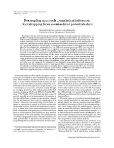
the process dynamics and related production parameters. The length of a segment is not necessarily coinciding with the length of the whole cycle as well as to those of the other segments. This is why a homogenous resampling is avoided and no reliable results can be obtained. In this contribution a feature-based resampling method is proposed, which requires the definition of reliable features of the signal. Discrete Wavelet Transform (DWT) [2] is used to locate a reliable set of features which is used as signal dividers specifying the segments to be resampled. The time series vectors of the sensor data considered in this paper measured from a real industrial example (Fig. 1) comprise the process cycles in a periodic nature of the signals [3]. A complete cycle of the considered production machine comprises actions of moving cylinders with different characteristics (Fig. 2). The sensor data include vibration velocity (V) and vibration acceleration (A) signals in addition to other system specific measurements. Vibration measurements are widely used in monitoring to support machinery maintenance decisions. The vibration velocity signal is a crucial variable to measure medium frequencies (until about 1 kHz), where the failure induced results from fatigue and wear out of surfaces. On the other hand, acceleration signals are more relevant in extracting transient, process-related, or impulse-like incidents, where the localized high frequencies are dominating for short times. Two other measurements are included in the example’s sensor data; the system hydraulic pressure (P) and the piston displacement of the monitored parts (D). Combining system hydraulic pressure and piston displacement provides implicit information about the friction and hence the tribological condition of the parts surfaces. Sys. pressure
3000
400 300 200
Disp.1
100
2500
0 -100
0
1000
2000
3000
4000
5000
6000
7000
8000
9000
Disp.3
10000
Displacement 3000
2000
1000 0 0
1000
2000
3000
4000
5000
6000
7000
8000
9000
10000
Vibration acceleration 1500 1000 500
Signal value
2000
Sys. pressure
1500
1000
Disp.2 Outlet
0 -500
500 0
1000
2000
3000
4000
5000
6000
7000
8000
9000
10000
7000
8000
9000
10000
Vibration velocity 4000 3000
0
Segment 1 starts here
2000 1000 0 -1000
0
1000
2000
3000
4000
5000
6000
Segment 16 ends here
Segment 7
-500
Time
Time
Figure 1. Raw data sample (example)
Figure 2. Machine operation cycle (example)
CLASSIFICATION INDICATORS In order to apply a successful classification process, the data must be prepared by careful transformation to extract the classification indicators. Redundant information should be excluded to avoid deterioration of the accuracy. Accordingly, the classification indicators containing the useful information should be presented in a recognizable structure suitable for classification, which is referred to as features. For classification purposes, the time series vectors of the sensor data (Fig. 1) do not conform to the cyclic nature of the considered machine. The classification indicators are the indicators of the system states to be classified, and these indicators might represent the process cycle as well as parts of it. As an example, Fig. 3 shows the vibration velocity of the operation cycles before and after a machine part
2
replacement. It can be seen, considering the signal intensity, that more classification indicators are located at the beginning of the cycles. In the case that classification is applied directly to the time series vectors, the other parts of the cycle will deteriorate the efficiency of the classification (Fig. 4). This is because no considerable difference between these points can be observed according to the different machine states. In the presented example, extraction of the operation cycles of the machine is a preliminary step for further extraction of features. Furthermore, it is important for the purpose of study to divide the process cycle into data segments. The operation cycle comprises actions of moving cylinders, and these actions have different importance, different shape, and accordingly, different characteristics of related real signals. Additionally, these actions have to be treated independently. Here in the example the machine cycle is divided into 16 data segments, (Fig. 2) each data segment has similar characteristics in all cycles. All these data segments of the machine process would give information about the behavior of the machine; however, some data segments are more informative and have more classification indicators than others. To recognize the segments which have more classification indicators, a feature space representing the two states of the machine is constructed using a training data set in the form of time series. In the feature space the points with the highest separability of the system states (the separable points in Fig. 4) are detected and re-allocated to the time series vector to specify the best candidate segments for classification. The data segments 1214 are found to be the best candidates to be considered.
Figure 3. Local changes in the cycles (example)
Figure 4. Local classification indicators (example)
FEATURE EXTRACTION OF OPERATION CYCLES In this section the proposed approach of feature based resampling is presented and applied along with other usual approaches for comparison purposes. Zero padding and homogenous resampling approaches For construction of the feature matrix as classifier input, cycles with constant lengths are required. Padding with zeros is an alternative method providing that changes in length are limited which is not the usual case in reality. Because of the reliability of the solution deteriorated by zero padding, in the presented example the zero padding is applied only for comparison purposes of the time series signals and their combinations. In order to consider cycles with equal lengths, a process of homogenous resampling is applied to the cycles. In this case the most usual length of the cycles is used as target length. The problem of this approach is that the lengths of the cycle
3
segments are not coinciding with the length of the cycles (Fig. 5). It is usual to have longer cycles with shorter individual segments. 300
Different lengths of cycles
200
Vibration acceleration
Features 100
0
-100
-200
-300
-400 0
10
20
30
40
50
60
70
Time
Figure 5: Cycles with different lengths (example)
Wavelet Transformation In wavelet analysis [2], signals are decomposed into wavelets of varying durations. These wavelets represent localized vibrations of a sound signal or localized variations of image details. Wavelets are used in a wide variety of signal processing tasks such as compression, removing noise, or enhancing recorded sound or image in various ways. Wavelets-based approaches are widely used in classification and recognition tasks as feature extraction tools [4, 5]. The performance of the wavelets is proved to be more flexible than other usual approaches such as STFT transform, where the size of the analysis window is restricted for all frequencies [6,7]. S
A
D1
A1
Lowpass Signal
Filters
A2
D2
D Highpass
A3
S1
Figure 6a: Discrete wavelet transform
D3
S2
S3 S4
Figure 6b: Wavelet decomposition tree
Figure 6c: Wavelet packet transform
Wavelet analysis is characterized with scales as function of frequencies and positions as function of time. It is also often characterized with approximations and details. Approximations (A in Fig. 6a) are the high-scale, low-frequency components of the signal, whereas details (D in Fig. 6a) are the low-scale, high frequency ones. Basically, the original signal is transformed into two sub-signals by two complementary filters (Fig. 6a). This process is iterated in the discrete wavelet analysis for successive approximations to realize the wavelet decomposition tree (Fig. 6b). In the reconstruction process the original signal is rebuilt by using the sub-signals (selectively in case of denoising) without loss of information. In the wavelet packet (WPT) analysis (Fig. 6c) the approximations as well as the details of the signal are successively decomposed into sub-signals. This leads to more possible decompositions and accordingly more possible representations of the original
4
signal; however the amount of information and the component selection process for reconstruction require more efficient techniques than those used for DWT. Entropy and energy approaches are used in combination with WPT. Energy can be used as a measure of the strength of a signal and equals to the sum of square of the signal magnitude, whereas entropy of the signal is a measure of randomness and uncertainty and used to describe the complexity of the system. Entropy and energy measures are used to detect the similarity between streams of data [8,9,10]. Signal
[S1....S8]
Input data of SVM
Energy or
WPT shannon entropy
[E1.....E8] or [H1.....H8]
Figure 7: The WPT energy and entropy
In the presented example of the cyclic data, the extracted cycle segments representing a cycle (signal S in Fig. 6c) are decomposed by WPT into different frequency bands using 6 depth Daubechies db4 wavelet. A group of sub-signals (AAA3 to DDD3 in Fig. 6c) is generated ranging from the low frequencies to the high frequency band. The different combinations of A and D indicate the position of nodes. Each node represents a certain degree of signal characteristics. The Shannon entropy and the total energy of each band signal are calculated (Fig. 7). The wavelet packet entropy or energy values on different frequency bands construct the feature vector, which reflects the information distribution of signals in frequency bands and used as the input vector to the SVM. Since one sub-signal corresponds to one entropy value or energy value, the advantage of combining WPT and entropy or energy measures is to have the length of the feature vector decoupled from the length of the original cycle. This means that different lengths of input cycles give a constant structure of the feature vector. On the other hand, since one sub-signal corresponds to one entropy or energy value, the feature vector contains only the information on frequency bands, i.e. these two methods only focus on describing the change in frequency domain. Feature-based Resampling Method In the case that two signals do not have the same form but the same entropy or energy values, difficulties in generalizing the solution with respect to the reliability of such high level of signal abstraction occurs. In the case of WPT and DWT, the length of the decomposed signals is related to the length of the original signal. In the presented example of cyclic signals, it can be seen from Fig. 7 that the cycle signals, which are usually of different lengths, have similar characteristics and type features. A resampling based on reliable signal features (nodes) is proposed to build the feature vector of the classifier. On the other hand, because of the noise and disturbances, it is sometimes difficult to detect features in the original signal which are similar in form and number in the cycles regardless of the state of the system.
5
Resampling of cycles decomposition
S 300
Different lengths of cycles
6 4
200
D1
A1
2 1
3
5
6
A2
4
D2
Cycle 2 2
20
0
-100
-200
-400 0
3 10
Original features
100
-300
5
1 0
Vibration acceleration
Detected features
Cycle 1
30
40
50
60
70
A3
10
20
30
40
50
60
70
Time
D3
Original signal of cycles S1
S2
S3 S4
Figure 8: Signal reconstruction in DWT and resampling
As the noise and disturbance are random, selective reconstruction of sub-signals in DWT can be applied to denoise the signal and detect the reliable features for resampling. Another possibility is to detect these features in the reconstructed signal from the selected components of the DWT and divide them into segments (6 segments in Fig. 8) and considered as the keys for the process of resampling (Fig. 8). In this way the time domain of the signal is changed and the corresponding information related to the time is disturbed. To solve this problem, the original positions of the discrete points in the reconstructed signal are stored in a matrix added to the input matrix of the SVM classifier. Here three level Daubechies db4 wavelet is used in the DWT decomposition. Signal comb. A P V D A-P A-V A-D P-V P-D V-D A-P-V A-P-D A-V-D P-V-D A-P-V-D
Table 1. Resulted classification accuracies Zero Homog. WPTWPTpadding res. Entropy Energy 94.54 % 86.21% 94.42 % 95.75 % 91.56 % 83.35% 83.89 % 89.05 % 96.96 % 93.01% 94.67 % 94.65 % 93.66 % 85.33% 88.78 % 92.89 % 95.53 % 92.68 % 93.64 % 97.36 % 93.17 % 90.15 % 96.06 % 92.26 % 94.48 % 97.14 % 93.23 % 93.32 % 95.41 % 89.51 % 91.68 % 97.34 % 92.78 % 95.17 % 97.44 % 93.44 % 90.15 % 96.23 % 92.18 % 92.96 % 97.67 % 93.02 % 94.29 % 97.44 % 92.82 % 95.24 % 97.76 % 93.45% 94.53 % 95.48 %
Feature-based resampling 94.35 % 97.50 % 96.79 % 95.17 % 94.67 % 96.42 % 94.85 % 96.80 % 98.56 % 97.11 % 96.87 % 94.95 % 97.00 % 97.02 % 97.32 %
CLASSIFICATION AND RESULTS A support vector machine classifier is applied to classify the states of the presented experimental example. The SVM method introduced by Cortes and Vapnik [1], is based on statistical learning theory and considered as one of the best techniques used in the field of pattern recognition. The learning problem setting of SVM [11] is to find the unknown nonlinear dependency mapping between the high dimensional
6
feature matrix and the output vector using the concept of maximum margin for better generalization. A decision function is used to classify the unknown data points according to the position and distance from the separating hyperplane (Fig. 9). Two classes are defined to train the SVM classifier [12]; the first one is the state before material change (old part), and the second is the state after material change (new part). A training data of 200 cycles, 100 cycles each class, were taken randomly from 4 places of the data. A linear kernel is considered because of the high number of attributes. The test set has a size 15874 cycles. The resulting classification accuracies for the four machine parameters (A, P, V, and D) and their possible combinations, using the different approaches discussed above are presented in Table 1. As mentioned before; the results of the direct application are added only for comparison because of the lack in the solution flexibility which results from the zero padding. In general, it can be seen that the results of the feature-based resampling are better than those of entropy and energy WPT. Additionally, the combination of signals improves the accuracy and the highest combination accuracy (P-D: 98.56%) is achieved by using the feature-based resampling approach. Optimal hyperplane
X2
State 1
Maximum margin
State 2
X1
Figure 9: Support vector machine (Feature space)
The resulting classification accuracies for the possible combinations of the DWT sub-signals (i.e. Approximations (Ax) and Details (Dx)) extracted from the four machine parameters (A, P, V, and D) are presented in Table 2. The results are based on the feature based resampling approach with and without consideration of the original positions (With/Without position) after resampling. Original positions are considered by connecting the two matrices of the resampled cycles and the original positions together. It should also be mentioned that the connected position matrix in Table 1 is optimized by a weighting factor in the feature matrix in order to improve the accuracy of the solution. No weighting factor was applied to the results in Table 2. It can be seen from Table 2, that the accuracy of classification is improved by considering the position information. It can also be seen that the optimal level for the Signal A
P
Table 2. Resulted classification accuracies of DWT components DWT Without With Signal DWT Without combination position position combination position A3 83.77% 83.85% V A3 94.00% A3+D3 87.63% 87.75% A3+D3 94.25% A3+D3+D2 90.31% 90.39% A3+D3+D2 94.37% A3+D3+D2 90.67% 90.70% A3+D3+D2 94.39% +D1 +D1 A3 92.33% 93.15% D A3 93.97% A3+D3 94.10% 94.21% A3+D3 92.72% A3+D3+D2 93.48% 93.81% A3+D2 91.57% A3+D3+D1 92.93% 93.31% A3+D1 91.95%
7
With position 94.01% 94.27% 94.38% 94.48% 95.17% 93.03% 91.78% 92.20%
classification (DWT combination) is different from machine parameter to another. This means that the extracted segment nodes, which not necessarily depend on some underlying system dynamics, are not only based on approximation indicatives. They are also based on details as well.
CONCLUSION In this work a feature-based resampling approach for industrial processes with periodic data is presented. The approach is used for fault classification and diagnostic purposes and based on the DWT to locate a set of reliable features which is used as signal dividers specifying the segments to be resampled. A real industrial example of process cycles with periodic nature of signals is presented to demonstrate the efficiency of the approach compared to other usual approaches. It can be shown that the results of the feature-based resampling are significantly better than those of entropy and energy WPT with considering preserving the position information. It can also be shown that the optimal level of wavelet decomposition is different between machine parameters, and depend strongly on approximation and detail indicatives as well. REFERENCES 1.
Cortes, C.; Vapnik,V.: Support Vector Networks, AT & T Labs Research, 1995.
2.
Walker, J.: A primer on wavelets and their scientific applications. Chapman and Hall/CRC, 2008.
3.
Saadawia, M.; Söffker, D.: Wavelet-based SVM system for evaluation of wear states and remaining life time. In: Chang, F. (Ed.): Structural Health Monitoring 2011, Stanford University, Stanford, CA, Sept. 13-15, 2011, pp. 1349-1356.
4.
Koley, C.; Purkait, P.; Chakravorti, S.: Wavelet-Aided SVM Tool for Impulse Fault Identification in Transformers. IEEE Transactions on power delivery, Vol. 21, No. 3, July, 2006.
5.
Supangat, R.; Ertugrul, N.; Soong, W.; Gray, D.; Hansen, C.; and Grieger, J.: Broken rotor bar fault detection in induction motors using starting current analysis. European Conference on Power Electronics and Applications (EPE), Dresden, Germany, 2005.
6.
Lee, J.; Lee, S.; Kim, I.; Min, H.; Hong, S.: Comparison between short time Fourier and wavelet transform for feature extraction of heart sound. Proceedings of the IEEE Region 10 Conference, TENCON 99, Vol. 2, 1999, pp. 1547-1550.
7.
Canal, M.: Comparison of Wavelet and Short Time Fourier Transform Methods in the Analysis of EMG Signals. Journal of Med. Systems, 2010.
8.
Omerhodzic, I. ; Avdakovic, S. ; Nuhanovic, A. ; Dizdarevic, K.: Energy distribution of EEG signals: EEG signal wavelet-neural network classifier. International Journal of Biological and Life Sciences, 6:4, 2010.
9.
Zhang, A.; Yang, B.; Huang, L.: Feature extraction of EEG signals using power spectral entropy. International Conference on Biomedical Engineering and Informatics, 2008.
10. Coifman, R.; Wickerhauser, M.: Entropy-based algorithms for best basis selection. IEEE Transactions on Information Theory. Vol. 38, No. 2, march 1992. 11. Abe, S.: Support vector machines for pattern classification. Springer-Verlag, London, 2005. 12. Chang, C.C.; Lin, C.J.: LIBSVM: a library for support vector machines. Software available at http://www.csie.ntu.edu.tw/~cjlin/libsvm, 2001.
8