SCHOOL OF COMPUTER STUDIES ... Division of Computer Science ..... For P 6= 2Q (integer valued Q) it is, of course, not possible to pair up all proces- sors for ...
University of Leeds
SCHOOL OF COMPUTER STUDIES RESEARCH REPORT SERIES Report 93.25
A Two-Way Parallel Partition Method for Solving Tridiagonal Systems by
C Walshaw & S J Farr
D iv isio n of C o m p u te r S cien ce June 1993
Abstract The Parallel Partition Method for tridiagonal systems is described.
It is
noted that, in the local reduction phase, the inherent parallelism is not exploited to the full and so a Two-Way Parallel Partition Method is introduced. new algorithm results in a reduced system of order
P=2 0 1
compared to
This
P
0
1
previously and in particular for 4 processors, a much lower arithmetic count. Both versions are tested and the results compared.
1
Introduction
1.1 The Parallel Solution of Tridiagonal Systems Many nearest neighbour problems (for example those involving spatial nite di�erence approximations) have at their heart a tridiagonal matrix. Their sparsity pattern suggests that, for large values of n, such systems are ideal candidates for parallelisation. However, the common methods for solving tridiagonal systems, such as Gaussian elimination or matrix decomposition, tend to be inherently sequential in nature and as a result, this topic was one of the earliest subjects investigated in the eld of parallel linear algebra. Amongst the rst such schemes were those introduced by Stone in the early seventies, [10] & [11] employing a recursive doubling algorithm. Another method, odd-even cyclic reduction, was developed by Golub and stabilised by Buneman, [2] & [3], and since its rst introduction for symmetric constant coe�cient matrices it has been extended to general non-symmetric tridiagonal systems, [12].
Figure 1: Matrix transformation for the partition algorithm In 1981 Wang, [17], introduced what he called a new (partition) method. This has also been referred to as the spike algorithm as it proceeds by a completely parallel local Gaussian elimination to transform the system from a tridiagonal one into 1
a diagonal one with spikes or ll-ins at the inter-processor boundaries. With one communication at the end of this local reduction phase, the result is a global order P 0 1 tridiagonal system in terms of the boundary variables (the unknowns at the inter-processor boundaries). Figure 1 shows an example matrix before and after the elimination phase where the dotted lines represent the inter-processor boundaries and the bold 2 symbols are the coe�cients of the O(P 0 1) system. This reduced system can then be solved globally with, for example, cyclic reduction or two-way Gaussian elimination and nally the internal values calculated each as a linear combination of up to two boundary variables. A variant, the method of Sameh et al., [9] & [6], uses no communication in the reduction phase but results in a pentadiagonal matrix. However, in a generalisation to narrow banded systems, Johnsson has shown, [4], that the extra communication is valuable and preserves positive de niteness and a form of diagonal dominance (albeit not in the classical sense { see [16] for further discussion). The majority of these partition algorithms have a common structure and can be split into three distinct phases which shall henceforth be referred to as:{ 1. The reduction phase { variables are eliminated to reduce the system to with an associated matrix usually known as the reduced matrix.
O(P ),
2. The reduced system is solved. 3. The back-substitution phase { the full solution is constructed from the variables of the reduced system. Of these, phases 1 and 3 can be carried out almost completely in parallel with no interprocessor communication. Phase 2 necessitates solving a system with one unknown per processor and is inherently a sequential operation. Since di�erent algorithms can be used for phases 1 and 2 (phase 3 being determined by these) such schemes are best described as [L][G] algorithms where [L] denotes the local algorithm of phase 1 and [G] the global phase 2. The competing methods and their implementation on di�erent architectures have all been comprehensively reviewed by Johnsson in [5]. He shows that a hybrid GECR (Gaussian Elimination locally, Cyclic Reduction globally) algorithm has similar arithmetic complexity to the full cyclic reduction algorithm and that the best method therefore depends on communication considerations. This report gives a description of the partition method and then goes on to develop a new and more e�cient version. Operation counts are established for both to 2
demonstrate the e�ciency and nally a comparison of timings for the two methods is given.
1.2 The Algorithms Three algorithms are presented in this paper, a two-way matrix factorisation algorithm, the Partition Algorithm, and the new Two-Way Partition Algorithm (sections 2-4 respectively). Each will be derived for the solution of the order n tridiagonal system 2 2 3 3 32 b c d x 1 1 1 1 66 6 7 6 7 7 6 7 6 7 7 66 a2 6 7 6 7 7 6 7 6 7 7 66 6 6 7 7 .. 7 = 6 .. 7 ... ... ... 6 7 Ax � 6 � d: (1) . 7 . 7 6 7 6 7 66 6 7 6 7 7 6 7 6 7 cn01 7 64 6 7 7 7 4 5 4 5 56 an
bn
xn
dn
For the purposes of this paper it is assumed that A is diagonally dominant and hence that the LU matrix decomposition algorithm can be used to factorise any submatrix of A. The techniques presented should, however, work for A symmetric & positive de nite and a Cholesky type decomposition. Either matrix type is very important; for more general matrices a pivoting strategy may be necessary and on a distributed memory network this can add such a large communication overhead as to completely kill any speed-up achieved by parallel solution. For the global solve of the reduced matrix in phase 2 of the partition algorithm several techniques, such as two-way Gaussian elimination, cyclic reduction and recursive doubling, are possible. However, the characteristics of the machine used for testing (see section 5.1.1 and [15, section 3.1.2] & [5, theorem 5.2]), together with the possibilities for reuse of code suggested the use of two-way matrix factorisation as described in section 2. The operation counts are based on this choice. Throughout, the assumption is made that the n equations are distributed on a chain of P processors. Secondly it is assumed that n � P so that each node has m = n=P unknowns assigned to it. Superscripts are used to denote the processor a particular value is stored on and subscripts the position in a vector.
1.3 Operation Counts For each algorithm an operation count is given and follows the generally accepted approximations for making theoretical timing estimations, see for example [5]. The machine dependent parameters are de ned as:{ 3
= time for one oating point operation; +, 0, 2 or 4 sc = start-up time for each inter-processor communication def tc = time to transmit one number. For matrices with multiple right hand sides, or which remain constant throughout many iterations, much work can be saved by generating a matrix decomposition once and storing it. In the following sections the square brackets [ & ] denote operations which, for constant matrices, need only be carried out once, rather than at every iteration. Alternatively, for multiple right hand sides, the costs that are not in square brackets are those required for each right hand side. ta
2
def
def
A Two-Way Matrix Factorisation Algorithm
In general, the classical algorithms for the solution of tridiagonal systems (such as Gaussian elimination and matrix decomposition methods) employ a forward sweep down through the variables followed by a backward sweep up. Whilst apparently sequential in nature, they actually have an inherent parallel degree of two, [8, page 22]. That is to say, two processes can be applied concurrently with no overlap of work. As an example, the system could be partitioned into a upper and lower half with each assigned to a processor. Then the upper processor can sweep down through the upper partition whilst the lower processor sweeps up through its partition. After an exchange of information, simultaneous back-substitution on each processor commences outwards from the centre. Alternatively consider a tridiagonal matrix distributed over a chain of processors, with each processor holding one variable. In this case the factorisation can sweep in along the chain from both ends and then out from the centre. This is not a new idea and, for example, two-sided Gaussian elimination was introduced by Babuska, [1, section 5], and a technique referred to as twisted factorisation described in [14]. However since this method is central to the Two-Way Partition Algorithm described below, full details of the two-way factorisation process are given. Henceforth this algorithm will be known as Two-Way (T W ) Decomposition and for convenience, these letters will be also used to refer to the two factorisation matrices.
4
2.1 The Method Consider the tridiagonal system (1) and let q = n=2. Echoing the LU decomposition algorithm, A will be factorised into the matrix product T W , where 3 2 u 7 66 1 7 7 66 a2 u2 7 7 66 ... ... 7 7 66 7 7 66 aq uq 7 7 6 T =6 7 7 66 uq+1 cq+1 7 7 66 ... ... 7 7 66 7 66 un01 cn01 7 7 5 4 un
and
W
2 66 1 v1 ... ... 66 66 1 vq01 66 66 1 vq = 66 66 vq+1 1 66 vq+2 1 66 ... ... 66 4 vn
1
3 7 7 7 7 7 7 7 7 7 7 7 : 7 7 7 7 7 7 7 7 7 5
Thus, in the upper partition, = b1 ; ui = bi 0 ai vi01 ;
u1
= c1=u1 ; vi = ci =ui ;
v1
i
= 2; . . . ; q ;
and similarly in the lower partition, = bn ; ui = bi 0 ci vi+1 ;
un
= an =un ; vi = ai=ui ;
vn
i=n
0 1; . . . ; q + 1:
Now let W x = z;
(2)
so that Tz =
d:
Then in the upper & lower partitions respectively, = d1 =u1 ; zn = dn =un ; z1
= (di 0 ai zi01)=ui ; zi = (di 0 ci zi+1 )=ui ; zi
5
i = 2; . . . ; q ; i=n
0 1; . . . ; q + 1:
From (2) the two central equations are + vq+1 xq + xq
= xq+1 =
vq xq+1
zq ; zq+1 ;
and to solve these the partitions must exchange information; zq [and vq for time dependent matrices] must be passed to the lower partition and zq+1 [vq+1] passed to the upper partition. Then xq ; xq+1 can be calculated from (1 0 vq vq+1 )xq = (1 0 vq vq+1 )xq+1 =
0 vqzq+1; zq+1 0 vq+1 zq :
zq
(3)
Finally, back-substitution gives = xi =
xi
0 vixi+1; zi 0 vi xi01 ;
zi
i=q
0 1; . . . ; 1;
i = q + 2; . . . ; n:
2.2 Stability of the algorithm Suppose A is strictly diagonally dominant. Then it is well known that A is nonsingular and the matrix can be factorised into an LU product, see for example [18, pages 122-124]. In addition this factorisation is strongly stable. The T W algorithm essentially comprises of two LU decompositions and thus is well de ned in this event. The only possible problem arises in the division by (1 0 vq vq+1) in equation (3). However, a simple check shows that jvij < 1 for all i and hence the decomposition is stable. A proof of this property is presented in [15, section 3.3].
2.3 Operation Count The arithmetic costs of this algorithm are:{
�
for the decomposition [3q 0 2]
�
for the inwards sweep 3q 0 2
�
for the central calculation 3 + [2]
�
for the outwards sweep 2q 0 2
2.3.1
Two Processors
The communication for a two processor algorithm requires 1 communication start-up (assuming the processors can exchange data simultaneously) and the transmission of 1 + [1] numbers. 6
The total cost for two processors is therefore:{
f5q 0 1 + [3q]gta + 1sc + f1 + [1]gtc:
(4)
If communication costs are small and n large, this is almost a linear speed-up over f5n 0 4 + [3n 0 3]gta, the cost of the sequential LU algorithm. 2.3.2
n
Processors
If instead there are n processors each assigned to one of the variables then the communication cost is modi ed slightly. There are n 0 1 communication start-ups; q 0 1 each for both inward and outward sweeps plus one extra for the central exchange. For each communication in the inward sweep and central exchange 1 + [1] numbers (zi & [vi]) are transmitted and in the outward sweep 1 number (xi) is transmitted. The total cost for n processors is therefore:{
f5q 0 1 + [3q]gta + f2q 0 1gsc + f2q 0 1 + [q]gtc: 3
(5)
The Partition Algorithm
Consider the solution of (1) on an array of P processors. The system can be distributed consecutively across the processors by partitioning it into P tridiagonal subsystems fS i : i = 1; . . . ; P g of order m interspersed with P 0 1 boundary equations fE i : i = 1; . . . ; P 0 1g. Thus m is de ned by the relation n = mP + P 0 1 and for simplicity it is assumed that n and P are such that m is an integer. In this way processor i is assigned the (relabelled) tridiagonal system ai1 e1xi01 + T i xi + cim emxi
= di
(S i )
where T i is a submatrix of A, e1 & em denote the standard unit basis vectors with [ej ]k = �jk and a11 = cPm = 0. The unknowns xi01 and xi denote the boundary variables and each of the boundary equations ai xim + bi xi + ci xi1+1
= di
(E i )
lies between the subsystems (S i) and (S i+1 ). The optimal assignment of (E i ) to a particular processor (to i or i + 1 for example) depends on the algorithm used in the phase 2 of the method.
7
3.1 The Method As described above the method has three phases: a local reduction phase to eliminate o�-diagonals in the subsystems (phase 1), the global solution of the reduced matrix for the boundary variables (phase 2), and (phase 3) the local back-substitution for the subsystem variables. 3.1.1
Phase 1
The (S i ) are rearranged to give xi as a linear combination of the two bounding variables xi01 and xi . Thus each processor `inverts' the matrix T i (for example via LU decomposition or Gaussian elimination) and uses it in (S i ) to obtain i = wi
x
0 rixi01 0 sixi
(S i )0
where = (T i)01 di ; i def = ai1(T i )01 e1; r i def s = cim (T i )01 em :
w
i
def
i01 and xi given by (S i )0 can now be substituted into The values for xi1, xi1+1 , xm m the boundary equations to yield
0airmi xi01 + (bi 0 aisim 0 cir1i+1)xi 0 cisi1+1xi+1 = di 0 aiwmi 0 ciw1i+1 and this can then be rewritten as the reduced O(P 0 1) tridiagonal system 2 2 3 3 32 1 ~b1 c~1 ~1 x d 66 6 7 7 6 7 6 7 7 6 7 66 a~2 6 7 7 6 7 6 7 7 6 7 66 6 7 6 7 .. 7 = 6 .. 7 ... ... ... 6 7 Rx � 6 : . 7 . 7 6 7 6 7 66 6 7 7 6 7 6 7 7 76 c~P 02 7 6 64 6 7 7 4 5 5 54 P 01 P 01 P 01 P 01 ~b a ~ x d~ The coe�cients are given by:{ ~i = a ~bi = c~i = d~i =
0airmi bi 0 ai sim 0 ci r1i+1 0cisi1+1 i 0 ci wi+1 di 0 aiwm 1 8
= 2; . . . ; P i = 1; . . . ; P i = 1; . . . ; P i = 1; . . . ; P i
01 01 02 0 1:
(E i )0
3.1.2
Phase 2
The second phase is the solution of this reduced system for the boundary variables. Again this can be accomplished in a number of ways, but, for the purposes of both the operation count and the results, the two-way matrix factorisation presented in section 2 is employed. 3.1.3
Phase 3
When each processor has the value of the two boundary variables of its local tridiagonal system it can then substitute them into (S i )0 to construct the solution. Thus the third phase can start locally as soon as the sweep has passed by.
3.2 Operation Count Assuming follows:-
LU
decomposition is used, the arithmetic costs of phases 1 & 3 are as Calculation Count Phase1 [Li ; U i ] [3(m 0 1)] i w 5m 0 4 [ri ] [4m 0 3] [si ] [m 0 1] Phase3 xi 4m
Notes
(1; 2) (1; 2) (2)
Notes:{ (1) Since T i ri = ai1 e1 and T isi = cim em , either the forward or the backward substitution (depending on the implementation of the LU decomposition) involves signi cantly fewer arithmetic operations than for a full right hand side such as i w . (2) Processor 1 need not calculate r1 and processor P need not calculate sP , so the cost of phase 3 for these two processors is just 2m. This may result in a saving for the algorithm since, being at either end of the chain for phase 2, they are the last to receive the boundary variables. However the saving is di�cult to generalise as it depends upon the size of m and on the relative costs of communication to arithmetic. Thus the total cost of vector operations in phases 1 and 3 is
f9m 0 4 + [8m 0 7]gta: 9
(6)
The calculation of the reduced matrix R and right hand side d~ requires 4 + [6] arithmetic operations per processor plus the transmission of 1 + [2] numbers. No communication start-ups are required as they can be included in the rst step of phase 2. This adds the cost
f4 + [6]gta + f1 + [2]gtc:
(7)
For phase 2, it can be seen from (5) that, writing q = (P 0 1)=2, the cost can be expressed as f5q + 2 + [3q]gta + f2qgsc + f2q + [q]gtc: (8)
The slight modi cation from (5) arises from solving 2q equations on 2q 0 1 processors. Thus, from (6)-(8), the complete cost, in terms of m and q , is
f9m + 5q + 2 + [8m + 3q 0 1]gta + f2q 0 1gsc + f2q + [q + 2]gtc:
(9)
3.3 Summary The algorithm given in this section shall henceforth be referred to as LU T W ; local LU decomposition, global T W decomposition. It is presented both to demonstrate this common strain of solver and to use as a building block to demonstrate the new version. In terms of n and P , the operation count can be summarised as P 0 1 communications with 17n=P + 4P arithmetic operations for time-dependent matrices and 9n=P + 5P=2 operations for constant ones. 4
The Two-Way Partition Algorithm
This method combines the algorithms of sections 2 & 3 to obtain a more e�cient algorithm for solving a tridiagonal system on an array of P processors. As a starting point consider the LU T W algorithm for P=2 processors and note that the local LU decomposition of phase 1 does not exploit the fullest parallelism possible. As seen in section 2 matrix factorisation of this type has a parallel degree of 2. Thus it is possible to assign each tridiagonal subsystem (S i ) to two processors and employ the T W algorithm for the local reduction. As a result a boundary equation is only required at every other inter-processor boundary and hence the reduced matrix is of order P=2 0 1 rather than P 0 1! A number of advantages manifest themselves:{ (i) It is immediate that the operation count in (9) is reduced. If n � P and P is small the gain is minimal, however, it can be seen that the algorithm LU T W is non optimal. 10
(ii) If implemented on a chain of processors with additional next-nearest neighbour connections, the number of communication start-ups can be reduced to P=2. This is possibly a signi cant saving. (iii) Algorithms of the form LU T W have often been demonstrated, see for example [5], [13] or [17], with a diagram showing a 4 processor version similar to gure 1 (page 1). These will usually have 3 (or sometimes 4) spikes or boundary ll-ins. However, using the T W algorithm for the rst phase results in only one ll-in { see gure 2. This has a consequence of reducing the operation count for phases 1 & 3 from 17n=P down to 14n=P [9n=P down to 7n=P for constant matrices] and is a signi cant saving for 3 or 4 processor implementations.
Figure 2: Two-way reduction for phase 1 using 4 processors It is also perhaps a more natural algorithm than LU T W since its restriction to two processors just results in the T W algorithm with an approximate arithmetic operation count of 4n, whereas the restriction of LU T W to two processors still results in boundary ll-ins and a count of 7n. This together with (iii) above makes it especially attractive for 4 or less processors, whilst (i) and in particular (ii) show general improvements.
4.1 The Method Again consider the solution of the tridiagonal system (1) on an array of P processors. For simplicity assume that P is even and that q = P=2. This time the system is distributed by dividing it up into q order 2m tridiagonal subsystems fS i : i = 2; 4; 6; . . . ; P g interspersed with q 0 1 boundary equations fE i : i = 2; 4; 6; . . . ; P 0 2g. Here m, the size of the tridiagonal block stored on each processor, is de ned by the relation n = 2mq + q 0 1. The subsystems are each assigned to two processors, so that each pair of processors i 0 1 & i store the system ai1e1xi01 + T i xi + ci2m e2mxi = di (S i ) 11
which is distributed by assigning the rst m equations to processor i 0 1 and the remaining m to processor i. Again the unknowns xi01 and xi denote the boundary variables and the boundary equation aixi2m + bi xi + ci xi1+2
= di
(E i )
lies in between the subsystems (S i ) and (S i+2 ). Phases 1 & 3 proceed in exactly the same way as in section 3.1, the only di�erence being that the calculation of wi , ri and si necessitates each pair of processors to use a T W factorisation with one communication exchange. Details of the matrix transformations and ll-in patterns of phase 1 are shown in gure 3. This shows the method implemented with two-way Gaussian elimination rather than decomposition but the concept is identical. The rst matrix shows the non-zeroes after the inward sweep and just before the communication exchange and the second shows them after the outward sweep. The inter-processor boundaries are marked with dotted lines.
Figure 3: Matrix transformations and ll-ins in phase 1 of algorithm T W T W
4.1.1
Phase 2
The reduced system is solved for the boundary variables, again by applying a T W decomposition to R. Since the order of the reduced system is q 0 1 (= P=2 0 1), the sweeps through the processor chain will employ half of the processors solely as communication relays. For machines with xed communication channels this may be the only possible implementation, but, if direct communication with next nearest neighbouring processors is possible, a further enhancement can be added. In this case, 12
if each boundary equation is stored on both sides of the inter-processor boundaries, the network can be divided into two independent parts, the even numbered processors, f2,4,. . . ,P 02g, and the odd numbered processors, f3,5,. . . ,P 01g, each with their own copy of the reduced matrix. Utilising the next nearest neighbour connections, both odd and even systems can then be solved simultaneously (with a T W decomposition) for a cost of approximately q communications start-ups, a considerable saving. Note that, as the outward sweeps nish, the values of x2 and xP 02 must be transmitted to processors 1 and P respectively to enable them to commence phase 3.
4.2 Stability of the algorithm Suppose A is strictly diagonally dominant. Then, since the T W algorithm is known to be stable, section 2.2, the only question is whether the reduced system inherits diagonal dominance from the full system. For the classical partition method, it is shown in [16] that this is indeed the case, regardless of the local reduction technique. Therefore, since a system reduced by local T W factorisation on P processors is identical to the reduced system after local LU factorisation on P=2 processors, it is readily seen that diagonal dominance is retained.
4.3 Odd Numbers of Processors
For P 6= 2Q (integer valued Q) it is, of course, not possible to pair up all processors for local T W factorisation. In this case one of the processors must employ LU decomposition whilst the rest use the two-way algorithm. This results in a reduced system of size (P 0 1)=2. Implementation is not di�cult as the T W code can be easily modi ed to do LU decomposition.
4.4 Operation Count The arithmetic costs of phases 1 & 3 are as follows:Calculation Count Phase1 [T i; W i ] [3m] i w 5m 0 1 i [r ] [4m 0 2] [ si ] [m] Phase3 xi 4m Notes:{ 13
Notes
(1) (1) (2)
(1) For processor i 0 1 the costs of ri and si are 4m 0 2 and processor i the costs are reversed. (2) Again for processors 1 and
P
m
respectively. For
the cost of phase 3 is just 2m.
In addition in phase 1 there is the cost of one communication exchange of 1 + [2] numbers (1 + [1] for the calculation of wi plus an extra [1] for one of the ll-ins). Thus the total cost of phases 1 and 3 is
f9m 0 1 + [8m 0 2]gta + 1sc + f1 + [2]gtc:
(10)
The calculation of the reduced matrix R and right hand side d~ again requires 4 + [6] arithmetic operations per processor plus the transmission of 1 + [2] numbers. A total of f4 + [6]gta + 1sc + f1 + [2]gtc: (11) For convenience in cost estimation for phase 2 assume that q is odd, so that the reduced system order q 01 is even. Then from (5) and writing l = (q 01)=2 = (P 02)=4 the cost can be expressed as
f5l 0 1 + [3l]gta + f2l 0 1gsc + f2l 0 1 + [l]gtc:
(12)
Finally at the end of phase 2, x2 must be transmitted to processor 1 and xP 02 to processor P , a cost of 1sc + 1tc : (13) Thus, from sums (10)-(13), the complete cost, in terms of
m
and l, is
f9m + 5l + 2 + [8m + 3l + 4]gta + f2l + 2gsc + f2l + 2 + [l + 4]gtc:
(14)
4.5 Summary Henceforth, using familiar taxonomy, this algorithm shall be referred to as T W T W { Two-Way decomposition locally, Two-Way decomposition globally. The operation counts can be summarised as P=2 + 1 communications with 17n=P + 2P arithmetic operations for time-dependent matrices or 9n=P + 5P=4 operations for constant ones. For 3 and 4 processor implementations this reduces to approximately 14n=P and 7n=P respectively, a substantial saving on the LU T W algorithm.
14
5
Results and Conclusions
Both algorithms have been implemented and timed extensively. Figure 4a (page 19) shows the cost in seconds for the solution of a system of size n = 50; 000 on varying numbers of processors. The timings presented here are for 4 to 32 processors in increments of 4. As a comparison, the cost of solving the same system using LU decomposition on a single processor is 1.886976 seconds which shows a maximum speed-up of 14.52 for T W T W on 32 processors. Since the arithmetic costs for T W T W (or any other partition method) are of the order 17n=P compared to 8n for LU , the maximum possible speed-up, neglecting any communication overhead, is about 8P=17 or 15.06 for 32 processors.
5.1 The Results The following results can be subdivided into di�erent cases dependent on P the number of processors. For 2 processors it is clear that the algorithm of choice is simply the T W decomposition, section 2, with no boundary variables. Since this does not fall into the category of an [L][G] (local-global) method no results are included here. The 4 processor case does have boundary variables but is somewhat di�erent to those with P > 4, section 4.5 and so these results are treated separately. 5.1.1
Hardware: The Meiko Computing Surface
The experiments were carried out on a Meiko Computing Surface consisting of 32 T800 transputers. This is a distributed memory MIMD machine with a con gurable network. The code was written in Meiko C with the message passing implemented using CSTools, [7]. Each processor has an on-board memory of 4MB and this limited the size of system that could be solved to approximately 23,500 equations per processor (i.e. 750,000 variables for 32 processors). The sequential LU code has much smaller memory requirements and runs with up to 62,000 equations. This latter memory limit made true speed-up gures impossible for systems of a larger size and so the results have been extrapolated to get approximate speed-up gures. 5.1.2
4 Processors
The operation counts show, sections 3.3 & 4.5, that the 4 processor T W T W algorithm has a lower arithmetic cost than LU T W (14n=P compared to 17n=P ) and this is clearly borne out by the actual timings. Figure 4b (page 19) shows the time for one solve for a number of di�erent sizes of system and it is clear that the n dependence 15
is smaller for T W T W . Figures 5a & 5b show the percentage reduction in time for T W T W over LU T W (i.e. 100 2 (tLUT W 0 tT W T W )=tLUT W ) and speed-up over the 1 processor LU algorithm respectively and for greater clarity these are drawn with n on a log10 scale. 5.1.3
More than 4 Processors
For P > 4 the arithmetic costs are approximately equivalent and it is the communication costs that are reduced by the T W T W algorithm. Figure 6a (page 19) shows the percentage reduction in time for T W T W over LU T W for 32 processors and varying sizes of system (again n is drawn on a log10 scale). Of course as the size of system increases, the arithmetical costs start to dominate and swamp any performance increase gained by communication. As a result, in all the tests, the percentage reduction in time appeared to reach an asymptotic limit of between 2-4% as the system size approached the maximum of 23,500 unknowns per processor. For smaller systems the gain in using T W T W over LU T W can be quite substantial, but this must be moderated by the overall e�ciency of the method. Figure 6b (page 19) show the corresponding speed-ups for the percentage di�erences shown in gure 6a. For example, if n = 10; 000 (log10 n = 4) T W T W is 17.7% faster than LU T W . However, for this system size T W T W is only 11.7 times faster than the sequential LU algorithm.
5.2 Conclusions The testing has revealed the T W T W algorithm to be generally more e�cient than LU T W . This is particularly noticeable for 4 or fewer processors where the algorithm is clearly seen to reduce the n dependence in the operation count. It is no more di�cult to implement than LU T W and the two experimental versions tested here used much of the same code. For large numbers of processors, the scalability issues of the algorithm lie in the global solve of the reduced system and hence the two-way partition method can be no worse than the original partition method. Future work in this area might involve the construction of an analogous algorithm for symmetric, positive-de nite systems with a Cholesky type matrix decomposition. In addition, further testing on di�erent machines is desirable and possibly the introduction of a di�erent algorithm such as Cyclic Reduction for the global solve. Acknowledgements
This algorithm was designed at the Mathematics Department, Heriot-Watt University, Edinburgh and bene ted greatly from the help of Dr. D. B. Duncan. 16
References
[1] I. Babuska. Numerical stability in problems of linear algebra. SIAM J. Numer. Anal., 9:53{77, 1972. [2] O. Buneman. A compact non-iterative Poisson solver. Tech. Rep. 294, Stanford University Institute for Plasma Research, Stanford, CA, 1969. [3] B. Buzbee, G. Golub, and C. Neilson. On direct methods for solving Poisson's equations. SIAM J. Numer. Anal., 7:627{656, 1970. [4] S. Lennart Johnsson. Solving Narrow Banded Systems on Ensemble Architectures. ACM Trans. Math. Soft., 11:271{288, 1985. [5] S. Lennart Johnsson. Solving Tridiagonal Systems on Ensemble Architectures. SIAM J. Sci. Stat. Comput., 8:354{392, 1987. [6] D. H. Lawrie and A. H. Sameh. The Computation and Communication Complexity of a Parallel Banded System Solver. ACM Trans. Math. Soft., 10:185{195, 1984. [7] Meiko Ltd., Bristol. Meiko CS Tools Manual, 1989. [8] James M. Ortega. Introduction to Parallel and Vector Solution of Linear Systems. Plenum Press, New York, 1988. [9] A. H. Sameh and D. J. Kuck. On Stable Parallel Linear System Solvers. J. ACM, 25:81{91, 1978. [10] Harold S. Stone. An E�cient Parallel Algorithm for the Solution of a Tridiagonal Linear System of Equations. J. ACM, 20:27{38, 1973. [11] Harold S. Stone. Parallel Tridiagonal Equation Solvers. ACM Trans. Math. Soft., 1:289{307, 1975. [12] Paul N. Swarztrauber. A Parallel Algorithm for Solving General Tridiagonal Equations. Math. Comp., 33:185{199, 1979. [13] Paul N. Swarztrauber and Roland A. Sweet. Vector and Parallel Methods for the Solution of Poisson's Equation. J. Comput. Appl. Math., 27:241{263, 1989. [14] H. A. van der Vorst. Large tridiagonal and block tridiagonal linear systems on vector and parallel computers. Parallel Comput., 5:45{54, 1987. 17
[15] C. H. Walshaw. Parallel Algorithms for Large Sparse Systems of Di�erential Equations. PhD thesis, Heriot-Watt University, 1991. [16] C. H. Walshaw. Diagonal Dominance in the Parallel Partition Method for Tridiagonal Systems. (submitted for publication), 1993. [17] H. H. Wang. A Parallel Method for Tridiagonal Equations. ACM Trans. Math. Soft., 7:170{183, 1981. [18] Burton Wendro�. Theoretical Numerical Analysis. Academic Press, New York, 1966.
18
1.1
1.6 "LUTW" "TWTW"
1
1.4 0.9 1.2 0.8 1 time/s
time/s
0.7 0.6
0.8
0.5 0.6 0.4 0.4 0.3 0.2
"LUTW" "TWTW"
0.2 0.1
0 0
5
10
15
20
25
30
35
0
10000
20000
30000
P
40000 n
50000
60000
70000
80000
Figure 4: Timings results for (a) n=50,000 & (b) P=4
28
2.6
26
2.4
24 2.2 22 speed-up
% reduction
2 20
18
1.8
1.6 16 1.4 14 1.2
12
10
"LUTW" "TWTW"
1 2
2.5
3
3.5 log n
4
4.5
5
2
2.5
3
3.5 log n
4
4.5
5
Figure 5: Results for 4 processors
50
16
45 14 40 12 35
speed-up
% reduction
10 30 25
8
20 6 15 4 10 2
"LUTW" "TWTW"
5 0
0 2
2.5
3
3.5
4 log n
4.5
5
5.5
6
2
2.5
3
Figure 6: Results for 32 processors 19
3.5
4 log n
4.5
5
5.5
6