Proceedings of the 8th World Congress on Intelligent Control and Automation July 6-9 2010, Jinan, China
A UKF Algorithm Based on the Singular Value Decomposition of State Covariance* Yulong Ma and Zhiqian Wang
Xingang Zhao, Jianda Han and Yuqing He
State Key Laboratory of Robotics, Shenyang Institute of Automation, CAS, Shenyang Graduate School of the Chinese Academy of Sciences, Beijing China
State Key Laboratory of Robotics Shenyang Institute of Automation, CAS Shenyang, Liaoning Province, China
{mayulong & wangzhiqian}@sia.cn
[email protected]
Abstract—One of the existing problems of General UKF is the stability problem due to the strong nonlinearity and the complexity of the system. When the algorithm can’t ensure the state covariance to be positive semidefinite, the precision will be decreased or even general UKF will be halted. Based on the singular value decomposition of state covariance, this paper proposes a modified UKF algorithm which can enhance the state covariance to be positive semidefinite. Comparing to the general UKF, the SVDUKF algorithm releases the condition of the positive semi-definite of state covariance. Numeric simulation experiments demonstrate the effectiveness of the algorithm. Index Terms - diagonal similar decomposition, symmetrical sample UKF, stability, positive semidefinite
o
I. INTRODUCTION
nline estimation technique aims mainly to obtain high precise states or parameters of a dynamic system with a set of noisy measured signals. Linear Kalman filter (KF) provides acceptable solutions in many situations [24]-[26]. However, in a larger of real applications, such as robots, industrial process, and even economy systems, the evolution of systems is governed by nonlinear functions, and this make the validity of KF is dropped greatly [27]. Thus, nonlinear estimation now constitutes an interesting and growing research area. In the past decades, many approximate optimal nonlinear estimation methods, including the extended Kalman filter (EKF) and the unscented Kalman filter (UKF), have been developed and applied to all kinds of practical nonlinear systems. Although EKF, which generalizes KF method to nonlinear systems by linearizing the nonlinear functions using Taylor series expansions, is most commonly used in real applications, it also exhibits several severe disadvantages, e.g. heavy computational burden due to the Jacobian Matrix and poor estimation precision for systems with high nonlinearities. In order to improve the performance of EKF method, researchers proposed a new KF based nonlinear estimation strategy – UKF[1]-[3]. UKF can deal with nonlinearities better on the basis of unscented transform (UT), a mechanism for propagating mean and covariance through a nonlinear transformation. It has been shown that UKF can approximate the posterior mean and covariance of the *
Gaussian random variable with a second order accuracy[15]. This makes UKF have higher precision than EKF algorithm. In recent years, UKF has obtained extensive attentions, and many researches on the performance of UKF can be found. These research works can be divided into two parts: 1) algorithm improvement; 2) applications. [8]-[12] present the applications of UKF algorithm in all kinds of fields. Such as, Chen et al. [8] studied UKF parameters estimation based on nonlinear observation and nonlinear kinetics model; Yamakita et al. [11] compared the recursive least squares, adaptive observer, EKF and UKF with a conclusion that the smaller error and higher precision algorithm is UKF; Ge Zhe-Xue et al. [12] brought forward a fault detect method based on UKF; UKF has been also introduced to the aircrafts modeling [9]. Besides the application researches, many researchers try to improve the performance of nominal UKF algorithm and many new version UKF algorithms are brought forward. For example, in 2001, square root UKF [13] was proved by Van der Merwe and Wan that the numeric stability and parameter estimation efficiency was higher (for special situation of parameter estimation is O(L2)). K. Xiong[15] proposed a revised UKF which could reach Cramér–Rao lower bound (CRLB) with a certain conditions. Song Qi [4] could estimate the covariance of noise online with the proposed Adaptive UKF (AUKF). Although UKF has been the focus of research of estimation online, there are still some to be improved with the algorithm. When the state covariance matrix is negative semidefinition, the estimation of states and outputs maybe complex, which is not consistent with the measurement. In this paper, a modified UKF, which is based on singular value decomposition, is proposed to ensure the positive semi definition of the state covariance matrix. Details of the modified UKF, proof of singular value decomposition of symmetrical matrix are presented in Section III. A brief mathematical formulation of the UKF is given in Section II. In Section Ⅳ discuss the numeric simulation. Section Ⅴ is the conclusion.
This work was supported by National Natural Science Fund of China (Grant No. 60705028, 60775056).
978-1-4244-6712-9/10/$26.00 ©2010 IEEE
5830
II. GENERAL UKF ALGORITHM
noises,
⎧ xk = f ( xk −1 , uk ) + vk (3) ⎨ ⎩ yk = Hxk + wk n r p where, xk ∈ R is the states vector, uk ∈ R and yk ∈ R are the input and output vectors at time instant k , respectively. vk and wk are the process noise and measurement noise
A. Unscented transformation (UT) Since UKF is based on the UT technique, a mechanism for propagating mean and covariance through a nonlinear transformation. We will first introduce the basic idea of UT. The unscented transformation (UT) is to calculate the statistics of a random variable which undergoes a nonlinear transformation [23]. Consider a random variable x (dimension N), which has mean x and covariance P, propagating through a nonlinear function, y = g(x). To calculate the statistics of y, matrix x of 2N+1 sigma points should be calculated as follow:
⎧x 0 = x ⎪ ⎨ x i = x + ( ( N + λ ) P )i ⎪ ⎩ x i = x + ( ( N + λ ) P )i − N
i = 1,..., N
E[vk ] = 0, E[ wk ] = 0, E[ wk wTj ] = Rk δ kj , E[vk vTj ] = Qk δ kj (1)
i = N ,..., 2 N
⎧ m λ ⎪ w0 = N + λ ⎪ λ ⎪ c + (1 − α 2 + β ) ⎨ w0 = N +λ ⎪ 1 ⎪ m c …, i = 1, 2N ⎪ wi = wi = 2( N + λ ) ⎩
such that
Here, we suppose that
each other. Nominal UKF algorithm for the associated noisy nonlinear system is described as follow, 1) Initialization
⎧⎪ x0=E[ x0 ] ⎨ T ⎪⎩ P0 = E ⎡⎣( x0 − x0 )( x0 − x0 ) ⎤⎦ ⎧ m λ ⎪ w0 = n + λ ⎪ λ ⎪ c + (1 − α 2 + β ) ⎨ w0 = λ + n ⎪ 1 ⎪ m c …, 2n i = 1, ⎪ wi = wi = 2(n + λ ) ⎩
(2)
where λ = ( N + κ )α − N ,α is the constant to control the Sigma point distribution, κ is a scaling parameter which is usually set to 0, and β is nonnegative constant. These sigma vectors are propagated through the nonlinear function, 2
y i = g (xi ) i = 0,..., 2 N Then the mean and covariance of y is approximated by a weighted sample mean and covariance of the posterior sigma points
where λ
(6)
= n(α 2 − 1) ,α is the constant to control the
χ k −1= ⎡⎣ xk −1 , xk −1 + (n + λ ) Pk −1 , xk −1 − (n + λ ) Pk −1 ⎤⎦
2N
i =0
2N
Py ≈ ∑ wim (y i − y )(y i − y )T
(3)
A simple sketch map of the UT method is shown in Fig 1. mean y=g(x)
covariance UT mean
(7) 3) Time update
⎧ χ k*|k −1 = f ( χ k −1 , uk ) ⎪ 2n ⎪ xˆ wim χ i*, k |k −1 = ⎪ k |k −1 ∑ i =0 ⎪ 2n ⎪ c T * * ⎨ Pk |k −1 = ∑ wi ( χ i , k |k −1 − xˆk |k −1 )( χ i ,k |k −1 − xˆk |k −1 ) + Q i =0 ⎪ * ⎪γ k |k −1 = h( χ k |k −1 ) ⎪ 2n ⎪ m ⎪ yˆ k |k −1 = ∑ wi γ i ,k |k −1 i =0 ⎩
i =0
covarianc e
UT covariance g(·) Sigma points
(5)
Sigma point distribution, and β is nonnegative constant. 2) Computation of the Sigma points
y ≈ ∑ wic y i
mean
vk , wk , xk are not correlative to
(8)
Transformed Sigma points
4)Measurement update
Fig. 1 Unscented transform
B. UKF Algorithm Consider the following nonlinear system with addictive
5831
⎧ ⎪ Pyk yk ⎪ ⎪ ⎪ Pxk yk ⎪⎪ ⎨ Kk ⎪ ⎪ Pk ⎪ x ⎪ k ⎪ ⎪⎩
exist orthogonal matrixes U and V such that
2n
= ∑ wic (γ i , k |k −1 − yk |k −1 ) ⋅ (γ i ,k |k −1 − yk |k −1 )T + Q n
⎡Σ 0⎤ T M =U ⎢ ⎥V ⎣0 0 ⎦
i =0 2n
= ∑ wic ( χ i , k |k −1 − xk |k −1 ) ⋅ (γ i , k |k −1 − yk |k −1 )T
The equation (10) is called singular value decomposition [22], where
i =0
= Pxk yk Py−k1yk
Σ = diag(σ 1 , σ 2 , σ 3 , σ r ) , σ i (i = 1, 2, r )
= Pk |k −1 − K k Pyk yk K kT
are all the nonzero singular values of M.
= xk |k −1 + K k ( yk − yk |k −1 )
n× n
Lemma: if M ∈ R is a real symmetrical positive semidefinite matrix, it can be decomposed as
(9) The computational cost of the UKF algorithm is similar as the EKF, but computational precision is much higher. Furthermore the Jacobian Matrix of the system function needs not to be computed any more. To reduce the computation burden, the sequence UKF [16] is used, which is in the measurement stage equation (9) is replaced by following equation (10)
⎧ Pk0 = Pk , k −1 ⎪ 0 ⎪ xk = xk ,k −1 ⎪ i i −1 i i i i −1 ⎪ xk = xk + K k ( yk − H k xk ) ⎪ i i −1 iT i i −1 iT i −1 (10) ⎨ K k = Pk H k ( H k Pk H k + Rk ) ⎪ i i i i −1 (i = 1, 2, m) ⎪ Pk = ( I − K k H k ) H k ⎪ x = xm k ⎪ k ⎪ Pk = Pkm ⎩ i i Where, H k is the i − th column of H k , yk is the i − th element of the measurement yk , K k is the i
i − th column of K k , xki and Pki are the i − th circle of the state vector xk and state covariance matrix Pk respectively. Although UKF has been the focus of research of estimation online, it requires initial value of state covariance should be nonnegative definition [1]-[3], which limit the application of the method.
⎡∑ M =U ⎢ ⎣0 ⎡ Σ =U ⎢ ⎣ 0
positive diagnal element.
□Proof: Because M is symmetrical and nonnegative definite, the eigenvalues of M are all nonnegative and real. From the definition of the singular value we find that the singular values are its eigenvalues, that is σ i ( M ) = λi ( M ) . Thereby
σ i2 x = M T Mx = M 2 x = MMx = M λi ( M ) x = λi2 ( M ) x T
and the eigenvectors of M M are that of M. Supposed that U is the orthogonal matrix composing of orthogonal eigenvectors of M, and V = U , we can get equation (11), which is singular value decomposition of M. Supposed
⎡ Σ 0⎤ T S =U ⎢ ⎥U ⎣ 0 0⎦ where Σ = diag(σ 1 , σ 2 , σ 3 , σ r ) σ i (i = 1, 2, r.r ≤ n) are all the nonzero singular values of M. Decomposing matrix M, we get
⎡∑ 0⎤ T M =U ⎢ ⎥U ⎣ 0 0⎦ = SS
A. Singular Value Decomposition of Symmetrical Positive definite Matrix the
real
symmetrical
matrix
0⎤ T U 0 ⎥⎦
(12) 0⎤ T ⎡ Σ 0⎤ T ⎥U U ⎢ ⎥U 0⎦ ⎣ 0 0⎦ where U is the orthogonal matrix. Σ is a diagnal matrix with
III. SINGULAR VALUE DECOMPOSITION BASED UKF (SVD-UKF)
Given
(11)
M ∈ R n× n ,
MM ≥ 0 , it must be a symmetrical matrix and its eigenvalues are all nonnegative. Define
Then we get the equation (12).
□
T
σ i2 = λi ( M T M ) Then σ i is called singular value of M [22], and here must
B. Algorithm based on singular value decomposition of state covariance matrix From theorem above, the state covariance matrix P is decomposed to chose the sigma points, which approximate the posterior mean and covariance of the Gaussian random variable, propagating mean and covariance through a
5832
nonlinear transformation. Replacing the equation (7) of the UKF algorithm, the new measurement update in algorithm is
⎧[U , D,V ] = fsvd ( Pk −1 ) ⎪⎪ T (13) ⎨C = U (n + λ ) D U ⎪ ⎪⎩ χ k −1 = [ xˆk −1 , xˆk −1 − C , xˆk −1 + C ] 2 2 2 2 where, D = diag(σ 1 , σ 2 , σ 3 , σ n ) , σ i (i = 1, 2, n) are the singular values of P (including 0).
(
)
mv =−Dcos β +Y sin β + XT cosα cos β +YT sin β +ZT sinα cos β − mg(cosα cos β sinθ −sin β sinφ cosθ
−sinα cos β cosφ cosθ) α = q −tan β( pcosα +r sinα) + −L+ ZT cosα − XT sinα +mg(cosα cosφ cosθ +sinαsinθ) mvcos β q = ( LI 2 + MI 4 + NI5 − p 2 ( I xz I 4 − I xy I5 ) + pq( I xz I 2 − I xz I 4 − Dz I5 ) − pr ( I xy I 2 + Dy I 4 − I yz I5 )
Fsvd(·) is the function to get the eigenvectors and singular values of the matrix (·).
+q 2 ( I yz I 2 − I xy I5 ) − qr ( Dx I 2 − I xy I 4 + I xz I5 ) −r 2 ( I yz I 2 − I xz I 4 )) / ΔI
C. The qualitative analysis of the stability Only the nonpositive semidefinition situation of the state covariance matrix is analyzed qualitative. When the state covariance matrix P is positive semidefinition, the new algorithm is consistent with the general UKF algorithm. While the state covariance matrix has at least one eigenvalue with negative real part, the new algorithm will work automatically to change the one-step predicted state covariance matrix to
⎡ Σ 0⎤ T ⎡ Σ Pk −1 = U ⎢ ⎥U U ⎢ ⎣ 0 0⎦ ⎣ 0 ⎡Σ 0⎤ T =U ⎢ ⎥U ⎣ 0 0⎦ where, Σ = diag(σ 1 , σ 2 , σ 3 ,
σ n ) , σ i (i = 1, 2,
λi ( P ) = λi ( P)
pq( I xz I1 − I yz I 2 − Dz I3 ) − pr ( I xy I1 + Dy I 2 − I yz I3 ) +q 2 ( I yz I1 − I xy I3 ) − qr ( Dx I1 − I xy I 2 + I xz I3 ) −r 2 ( I yz I1 − I xz I 2 )) / ΔI
r = ( LI3 + MI5 + NI 6 − p 2 ( I xz I5 − I xy I 6 ) +
0⎤ T ⎥U 0⎦
pq( I xz I3 − I yz I5 − Dz I 6 ) − pr ( I xy I3 + Dy I5 − I yz I 6 ) −r 2 ( I yz I3 − I xz I5 )) / ΔI
n)
are the singular values of P (including 0). Although P ≠ P ,
p = ( LI1 + MI 2 + NI3 − p 2 ( I xz I 2 − I xy I3 ) +
. This will ensure the
sigma point belong to the real field and enhance the positive semidefinition of the state covariance matrix P, so it releases the requirement of the state covariance matrix and ensure the precision of the estimation. IV. NUMERIC SIMULATION Used a fighter as the background, a nonlinear system model is built to validate the new algorithm. In this paper, the fixed-wing UAV model is used to verify the feasibility and validity of the proposed algorithm. The nonlinear function is as follows,
θ = q cos φ − r sin φ φ = p + q sin φ tan θ + r cos φ tan θ ψ = r cos φ sec θ + q sin φ sec θ β = p sin α − r cos α + ( D sin β + Y cos β − X T cos α sin β + YT cos β − ZT sin α sin β + mg (cos α sin β sin θ + cos β sin φ cos θ − sin α sin β cos φ cos θ )) / (mv) h = v(cos α cos β sin θ − sin β sin φ cos θ − sin α cos β cos φ cos θ ) where XT,YT and so on are the corresponding parameters of the fighter. Compact above equations as:
x = f ( x, u , t ) + v(t ) y = x + w(t )
where,
u and
(14)
x = [V , α , q, θ , p, φ , r ,ψ , β , h]T is the state vector,
y
are input and output vectors respectively,
u = [δ H δ lf δ rf δ Aδ F δ R ]T . f is the nonlinear differential function. v (t ) and w(t ) are the independent white noises. Euler method is used to discretize the system
xk +1 = xk + Tf ( x, u, t ) + Tv(t ) yk = xk + w(t )
(15)
where, T is the step time of the simulation. The simulator is built on the matlab7.5, the two UKF algorithms are both
5833
realized, and only the real part of equation (7) of general UKF algorithm is used to ensure program running (This will deteriorate the performance of the filter greatly, as shown in our simulation results). The initial values of the simulator:
beata 0 real genest SVDest
-0.02 -0.04 -0.06 beata(rad)
T = 0.1
x0 = [550, 0.0891,0.0891, 0,0,0,0,0,0,9800]
T
-0.08 -0.1 -0.12
To prove the superiority of SVDUKF, the initial values of the algorithms are initialized
-0.14
xˆ0 = 0.8 x0 Pˆ0 = −diag ([35;1;1;1;1;1;1;1;1;300]2 )
-0.16
0
10
20
30
40 time(s)
50
60
70
80
Fig.4 Estimation of angle of side-slip
Q = 10−8 I
h 10000
R = diag ([1.5;0.0015;0.0015;0.0015;0.0015;
real genest SVDest
9000
0.0015;0.0015;0.0015;0.0015;60]2 )
8000 7000
V
6000
700
600
h(m)
real genest SVDest
5000 4000 3000
500
2000 V(m/s)
400
1000 0
300
10
20
30
40 time(s)
50
60
70
80
200
Fig.5 Estimation of height
100
Figure 2~5 indicate that when errors exist in initial estimation values and the state covariance matrix is the situation of nopositive semidefinition, the two algorithm work much differently. Tab.1 lists the MSE of some state estimation error. All the results indicate that SVDUKF improve the stability and converge of the algorithm, and release the requirement to the positive semidefinition of state covariance matrix. In the table GENUKF is represented the general UKF algorithm and SVDUKF is represented the SVDUKF algorithm.
0
0
10
20
30
40 time(s)
50
60
70
80
Fig.2 Estimation of velocity alpha 0.1 real genest SVDest
0.09 0.08 0.07 0.06 alpha(rad)
0
Tab.1 comparison of MSE
0.05
Method
V(ft/s)
0.04
GENUKF ―― SVDUKF 337.47
0.03 0.02
α
(°)
β (°)
h(ft)
1.032×10⁻⁴ 8.66×10⁻⁴ —— 5.78×10⁻⁷ 1.995×10⁻⁵ 9.74×10⁵
0.01 0
0
10
20
30
40 time(s)
50
60
Fig.3 Estimation of angle of attack
70
V. CONCLUSION
80
A modified UKF algorithm is proposed, which is based on the singular value decomposition of state covariance (SVDUKF). The proposed algorithm is proved to be superiority to the general UKF algorithm by the numeric simulation. The positive semidefinition can be ensured in SVDUKF algorithm, so it releases the requirement of the state covariance matrix and ensure the precision of the estimation. There is deduction of the algorithm as well as qualitative analysis in the paper.
5834
REFERENCES [1]
[2] [3]
[4]
[5]
[6] [7] [8]
[9] [10]
[11]
[12]
[13]
[14] [15] [16] [17] [18]
[19] [20]
[21] [22]
R. E. Kalman. A new approach to linear filtering and prediction problems. Transactions of the ASME--Journal of Basic Engineering, 1960, 82(Series D): 35~45 S. J. Julier, J. K. Uhlmann, H. F. Durrant-Whyte. A new approach for filtering nonlinear systems. The Proceedings of the American Control Conference, Seattle, Washington, 1995: 1628~1632 E. A. Wan, R. Van der Merwe. The unscented kalman filter for nonlinear estimation. Proceeding of the Symposium 2000 on Adaptive System for Signal Processing, Communication and Control (AS-SPCC), Lake Louise, Alberta, Canada, 2000 Qi Song , Zhe Jiang, Jianda Han. Noise Covariance Identification Based Adaptive UKF with Application to Mobile Robot Systems. 2007 IEEE International Conference on Robotics and Automation Roma, Italy, 10-14 April 2007 Yanling Hao, Zhilan Xiong, Feng Sun, Xiaogang Wang. Comparison of Unscented Kalman Filters. Proceedings of the 2007 IEEE International Conference on Mechatronics and Automation August 5 - 8, 2007, Harbin, Chinathe Yang.F, Pan.Q, Liang.Y, Cheng.Y, Liu.W. Survey of Sampling Nonlinear Filter. Proceedings of the 25th Chinese control conference, August, 2009, Harbin Heilongjiang. Peng.D, Guo.Y, Xue.A. An interacting multiple model algorithm for a 3D high maneuvering target tracking. Control Theory&Applications.Vol.25 No.5 Y. Q. Chen, H. Thomas, Y. Rui. Parametric contour tracking using unscented Kalman filter. Proceedings of the 2002 International Conference on Image Processing (ICIP 2002), New York, USA, 2002, (3): 613-616 M. C. VanDyke, J. L. Schwartz, C. D. Hall. Unscented Kalman filtering for spacecraft attitude state and parameter estimation. on line: http://www.aoe.vt.edu/~cdhall/papers/AAS04-115.pdf, 2004 C. Song, H. Sharif, K. Nuli. A UKF-based link adaptation scheme to enhance energy efficiency in wireless sensor networks. The 15th IEEE International Symposium on Personal, Indoor and Mobile Radio Communications, 2004, (4): 2483~2488 M. Yamakita, Y. Musha, G. Kinoshita. Comparative study of simultaneous parameter-state estimations. Proceedings of the 2004 International Conference on Control Applications, Taiwan, 2004, (2): 1621~1626 Zhexue Ge, Yongmin Yang, Xingwei Wang, Zheng Hu. New UKF-Based Method for Sensor Bias Fault Detection in Stochastic Nonlinear System. Chinese Journal of Sensors and Actuators. 2005, 18(4): 910~914 R. Van der Merwe, E. A. Wan. The square-root unscented Kalman filter for state and parameter-estimation. In Proceedings of the International Conference on Acoustics, Speech, and Signal Process, Salt Lake City , 2001: 3461-3466 Zhao Fu-cai, Yin Cheng-you, hang Li. Transformation Wavelet Based Unscented Kalman Filter and Its Application. Radio Communications Technology Vol134 No14 2008 K. Xiong, H.Y. Zhanga, C.W. Chanb. Performance evaluation of UKF-based nonlinear filtering. Automatica 42 (2006) 261 – 270 Hui-ping Li, De-min Xu, Jiang Li jun and Fu-bin Zhang.Sequence Unscented Kalman Filtering Algorithm. Industrial Electronics and Applications, 2008. ICIEA 2008. 3rd IEEE Conference. 1374-1378 Pan Quan, Yang Feng, Ye Liang, Liang Yan, Cheng Yong-mei. Survey of a kind of nonlinear filters—UKF. Control and Decision. Vo l. 20 No. 5 Simon Julier, Jeffrey Uhlmann, and Hugh F. Durrant-Whyte. A New Method for the Nonlinear Transformation of Means and Covariances in Filters and Estimators. IEEE TRANSACTIONS ON AUTOMATIC CONTROL, VOL. 45, NO. 3, MARCH 2000 Simon J. Julier. The Scaled Unscented Transformation. Proceedings of the American Control Conference Anchorage, AK May 8-1 0,2002 Simon J. Julier, Jeffrey K. Uhlmann. Reduced Sigma Point Filters for the Propagation of Means and Covariance Through Nonlinear Transformations. Proceedings of the American Control Conference, Anchorage, AK May 8-10,2002 Simon Uulier, Jeffrey K.Uhlmann. A general method for approximating nonlinear transformations of probability distributions. Oxford, OX1 3PPJ United Kingdom. 1st November, 1996. Yunpeng Cheng. Matrix theory (2nd edition). Northwestern Polytechnical University Press, 2004.
[23] S . J. Julier and J. K. Uhlmann. A New Extension of the Kalman Filter to Nonlinear Systems. In Proc. r?fAem.sen.ve: The 11th Inr. Symp. On Aerospuce/Dejence Sensing, Simulation and Controls., 1997.
[24] Li Ju, Zhao Fang. Analysis for Kaiman Filter Used in Digital Differential Protection of Transformer. Journal of Zhejiang University(Engineering Science), Vol.6, 1989 . [25] Ji Liangzhao. A Z80 Single Board Computer Used to Accomplish Kalman Filter of Measured Radar Data and Digital Display. Journal of National University of Defense Technology, Vol.4,1985. [26] Fang Jiancheng,Shen GongXun. An Adaptive Federated Kalman Filter and Its Application at GPS/DR Integrated Navigation System in Land Vehicle. JOURNAL OF CHINESE INERTIAL TECHNOLOGY, vol.6,No.4,1998 . [27] Youmin Zhang, Guanzhong Dai, Hongcai Zhang. The Development of Kalman Filter Aigrithm. CONTROL THEORY AND APPLICATION, Vol.12, No.5, 1995
5835