In the covariance equation (4) of the conventional Kalman filter, assume that the ..... [201 F.T. Luk, "Computing the singular value decomposition on the. Illiac IV.
-
WP13 1650
KALMAN FILTER ALGORITHM BASED ON SINGULAR VALUE DECOMPOSITION Liang Wang, Gaetan Libert and Pierre Manneback Department of Computer Science Faculte Polytechnique de Mons, Rue de Houdain 9 7000 Mons, Belgium
Abstract: This paper develops a new algorithm for the discrete time linear filtering problem. The crucial component of this algorithm involves the computation of the singular value decomposition (SVD) of an unsymmetric matrix - without explicitly forming its left factor that has a high dimension. The presented algorithm has a good numerical stability and can handle correlated measurement noise without any additional transformation. This algorithm is formulated in the form of vector-matrix and matrixmatrix operations, so it is also useful for parallel computers. Details of the algorithm are provided and a numerical example is given. I. INTRODUCTION
The Kalman filter [14] has been one of the most widely applied techniques in the area of modem control, signal processing, and communication applications. By using a state space model, it facilitates the estimation of the unknown state vector recursively for each new observation. It is considered an optimal estimator because it provides a minimum variance estimate. Discussion and applications on Kalman filter can be found in many literature. The following equations define a discrete time state space system: = @k+l,kXk+GkWk
(1)
where x ~ E ' Wis the state vector, %E%'" is the measurement vector, wreW is the disturbance input vector, vk€R" is the measurement noise vector, *+,.,~Wnx", G k ~ ' W xand r Hlr~%jnxs are the system matrices. The disturbance w, and noise v, are assumed to be zero mean Gaussian white noise sequences with symmetric positive definite covariance matrices Q, and &, respectively. Furthermore, sequences w, and v, assumed to be statistically independent. The Kalman filter is then described by the following recursive equations under assumptions that matrices G,, €&,Q, and Rkare known: Time extrapolation:
(4)
Measurement update:
K, = P,H,T(H,P,H,+R,)-'
S = PIn such that
P = SST
where S is obtained in triangular form by the well-known Cholesky decomposition. Although equivalent algebraically to the conventional Kalman filter recursion, the square root approach exhibits improved numerical precision and stability, particularly in ill-conditioned problems. The advances in square root filtering up to 1971 have been summarized by Kaminski, Bryson and Schmidt [15]. Subsequently, Carlson [6] and Bierman [5] have introduced strictly algorithmic approaches to the square root filtering. Bierman also introduced the idea of using a UDL decomposition of the covariance matrix in place of the square root decomposition. This is a decomposition of the sort P = UDUT
where D is a diagonal matrix and U is an upper triangular matrix with 1's along its main diagonal. This factorization does not require taking scalar square roots and is superior in most respects to the basic square root algorithm [21]. Both the square root and the UDUTdecompositions may result in numerically stable filter algorithms. But these formulations can only be used if one has single dimension measurements with uncorrelated measurement noise. Generally one does not have this in practice. To handle correlated measurement noise, additional transformations have to be used which increase the computation cost. Moreover, these formulations cannot be effectively implemented on vector processors because their designs are virtually serial in structure. Extensions of the Potter and the Bierman methods to the multiple measurement case have been devised by several researchers [1][3][18]. Especially, in a recent paper by Hotop [13], the author gives a fresh Kalman filter formulation which is based on a special Givens orthogonal transformation. Hotop's algorithm has been shown to be very useful for parallel computers. In the sequel of this paper we will present an SVD-based Kalman filter algorithm which has the UDUT formulation as in the Bierman method. Like Hotop's algorithm, our algorithm is also suitable for parallel computers, but it has a higher numerical stability than Hotop's and other previous algorithms.
U)
where Pk is the covariance of estimation uncertainty, superscript + refers to values after the measurement update, and & is the Kalman gain matrix. The major disadvantage of the Kalman formulation is that the matrix subtraction in Eq.(6), representing the reduction in uncertainty
CH3229-2/92/0000-1224$1.OO 0 1992 IEEE
due to the measurement, can yield a result P c that is computationally not positive definite (or, at least, nonnegative) -- a theoretical impossibility. To circumvent this difficulty, Potter [2] introduced the idea of using a square mot of the covariance matrix in the algorithmic implementation. This is a matrix
11. SINGULAR VALUE DECOMPOSITION AND
ITS
COMPUTATION One of the basic and most important tools of modern numerical analysis, particularly numerical linear algebra, is the singular value iecomposition. For a survey of the theory and its many interesting 1224
applications, see Vandewalle and De Moor [22]. The singular value decomposition of an m-by-n matrix A(m2n), is a factorization of A into a product of three matrices. That is, there exist orthogonal matrices UE 'Prn and VE 3""" such that
A where AE %"
=
UAVT, A
=
1:]
and S=diag(o,,...,or) with o1 L ... 2 or > 0 .
The numbers (J,,...,or together with or+,=O ,...,o,=O are called the singular values of A and they are the positive square roots of the eigenvalues of ATA. The columns of U are called the left singular vectors of A(the orthonormal eigenvectors of AAT) while the columns of V are called the right singular vectors of A(the orthonormal eigenvectors of A ~ A ) . It is known that the singular values and singular vectors of a matrix are relatively insensitive to perturbations in the entries of the matrix, and to finite precision errors [24]. Furthermore, since the (3,'s are, in fact, the eigenvalues of a symmetric matrix, they are guaranteed to be well-conditioned so that, with respect to accuracy, we are in the best of possible situations [16]. In practice, if ATA is positive definite then (8) can be reduced to
A
=
U!:] V T
where S is an n-by-n diagonal matrix. Especially, if A itself is symmetric positive definite then we will have a symmetric singular value decomposition A = USUT = UDZUT (10) In our filter algorithm derivation, (9) and (10) will be of particularly real interest. The standard method for computing (8) is the Golub-KahanReinsch SVD algorithm ([9] and [lo]), in which the Householder transformation is fxst used to bidiagonalize the given matrix and then the QR method to compute the singular values of the resultant bidiagonal form. Recently, with the advent of massively parallel computer architectures, two classical SVD computation methods, that is, Hestenes algorithm (one-sided Jocabi) [12] and Kogbetliantz algorithm (two-sided Jocabi) [17], have gained a renewed interest for their inherent parallelism and vectorizability (see a good overview written by Berry and Sameh [4] summarizing parallel algorithms for the singular value and symmetric eigenvalue problems). For illustration, Table I gives the computation flops of Golub-KahanReinsch algorithm (G-K-R), row-oriented Hestenes algorithm (RHestenes), column-oriented Hestenes algorithm (C-Hestenes), and Kogbetliantz algorithm (Kogbetliantz) for random n-by-n mamces A whose elements are uniformly distributed in the interval (0, 1)(An initial QR step is done before the SVD procedures are applied to A).
All algorithms are implemented in the MATLAB environment and ran on a PC 486 [23]. It can be seen that the Golub-Kahan-Reinsch algorithm is most computationally efficient on the sequential machine. However, this algorithm will become less attractive on a parallel processor [20], while Hestenes algorithm and Kogbetliantz algorithm will be of importance there. Our present Kalman filter formulation is based on Golub-KahanReinsch algorithm and ran on the sequential machine. In a future paper we will discuss its parallel implementation on a transputer network in which Kogbetliantz's two-sided Jocabi algorithm will be used. 111. NEW KALMAN FILTER FORMULATION Time Extrapolation Formulation In the covariance equation (4) of the conventional Kalman filter, assume that the singular value decomposition of P; is available for all 4 and has been propagated and updated by the filter algorithm. Thus, we have p i = U'D'Zu;T f k
Eq.(4) can therefore be written as
Our goal is to find the factors U,, and D,, from Eq.(ll) such that Pk+I=U,,D,,ZU,+,T, where U factors are orthogonal and D factors are diagonal. Provided that there is no danger of numerical accuracy deterioration, one could, in a brute force fashion, compute P,,, and then apply the singular value decomposition of symmetric positive definite matrix which is given by Eq.(lO). However, it has been shown that this is not a good numerical exercise [lo]. Instead we define the following (s+n)-by-n matrix
and compute its singular value decomposition
Multiplying each side on the left by its transpose, we have @k+l,kuk*Dk+TDk+
u;T@:+l>
+
G k / a / a T G l
TABLE I AVERAGE NUMBER OF FLOPS FOR DIFFERENT SVD ALGORITHMS
I
n
Trials
4 6 8 10 20 30 40
100 100 100 100 10 10 10
G-K-R 1480 486 1 10992 20573 149700 488670 1 136000
R-Hestenes
C-Hestenes
2607 10686 27841 57939 537220 1973400 4867800
2918 11839 31061 63972 601350 2119208 5 162000
I
Kogbetliantz 3412 14017 35489 7557 1 686890 2428400 5950600 I
1225
Lompanng two siaes or 4 4 1 ~ ) . we get vk'
Comparing the result with (1l), we find that vk' and 4' are just the U,, and Q+l we are looking for. Here we want to point out that the (s+n)-by-(s+n) orthogonal matrix Ut' and its transpose Uk'Tare not needed directly in our algorithm and it is not necessary to store or compute them explicitly. Measurement Uudate Formulation
D i = (Di)-' (21) In this manner, a new measurement update formulation has been obtained. The crucial component of the update, like that of time extrapolation, involves the computation of the singular value decomposition of an unsymmetric matrix - without explicitly forming its left orthogonal factor that has a high dimension. For the Kalman gain an alternative expression may also be derived. Beginning with Q. (7) we have
In the conventional Kalman measurement update, substituting Eq. (7) into (6) yields
pk+ = pk- pkH:(HkPkH:+$
I-'
HkPk
Insertion of P,+(Pc)-' and R;'R, will not alter the gain. Thus, & can be written as
(13)
To obtain the new measurement update result, we will require use of the well-known matrix inversion lemma, valid for positive definite NandM (N+BMB?-' = N-'-N-'B(B TN'iB+M-')-'B 'N-' It follows from this and (13) that
(P; I-'
We now use Q. (14) for (P,')-'
=
+
H:R;'H,
and get
(14)
Kk = P i H : q i
Applying the singular value decomposition of symmetric positive definite matrix to Pc and Pk,respectively, we may get (uk'Dk'2
Uk+T)-l = (ukD,'u:)-'
+ H:R;'Hk
There is no need to obtain a formula for the singular value decomposition of &. The state vector measurement update is given by
In (15) let
L,L;
=
R;'
(16)
Together with the time extrapolation described in the above section and the measurement update of the covariance matrix and the state vector described here, a new Kalman filter algorithm is formulated, and it is summarized in Fig. 1.
be the Cholesky decomposition of the inverse of the covariance Algorithmic Details matrix. If the inverse is available then there is no difficulty. If the covariance mamx q is known, but not its inverse, then the reverse In this section we provide a few details and references for the new Cholesky decomposition &RHT=R, 5"upper triangular, can be algorithm summarized in Fig. 1. found(see, for example, [ 111). It then follows that &=RH?-' is the (i) Determine initial U, and D,,. In practice, the initial Po is required Cholesky decomposition in (16). generally assumed to be diagonal, in which case we set U,=I and Now considering the Im+n)-bv-n matrix D,=P,. If Pois not diagonal then a symmetric QR algorithm [ 111 can be used to compute the U, and Po,and about 9n' flops are required. (ii) Update U: and .D: The key to this step is the construction of the (m+n)-by-n matrix
[L2"j
and computing its singular value decomposition, we have
Multiplying each side on the left by its transpose yields
Dk-' + U : H:Lk LIHk U k =
vk' 0,' 'vk'
(18)
Then EQ.(15) can be written as (
')-' ( D k + )
-'( U,' )-'
= ( U:)-'
vk'
4' 'vk'
U;'
and then its S V D computation. Because of the iterative nature of the SVD algorithm it is difficult to give a reliable flop count. In terms of Golub and Van Loan's estimate, forming the explicit matrix product and doing a standard SVD(inc1uding accumulating the U and V factors) using the efficient Golub-Reinsch algorithm requires 4(1n+n)~n+8(m+n)n~+9dflops. In our filter formulation, only the right SVD factor V is needed, so the practical flop count is 4(m+n)n2+8n3=4mn2+12n3.Furthermore, if we nonce the fact that the above matrix has the form 1226
Enter %, U, and Do (U, and Do are obtained from the SVD of Po)
Compute gain
&:
K~=U;D;~U:~H:L,L;
Fig.1. New Kalman filter recursive loop.
* * * o o o
* * o * o o
* * o o * o
(iv) compute the extrapolations ~ + l , ~ k + and l , Dk+,.?k+l can be directly computed from Eq. (3) with trivial flops. U,+, and D,, can be obtained from the singular value decomposition of the (s+n)-by-n matrix
* * o o o *
where * denotes the non-zero element of the matrix, then we can further reduce the computation flops to approximately 5mnz+10n3by bidiagonalizing this matrix using both Givens rotations and Householder reflections(Here we assume that m is less than n, as it often does in practical Kalman filter applications). In the above matrix, L is the Cholesky decomposition of the inverse of the m-by-m covariance matrix R,, and its computation requires 1/3 m’ flops. If the covariance matrix Rk is known, but not its inverse, then L can be obtained from the reverse Cholesky decomposition, with an additional 1/3 m3 flops for computing the inverse of the Cholesky factor[8]. Especially, if the covariance matrix Rk cannot be always guaranteed to be positive definite then the numerical reliable SVD algorithm can be used for computing its inverse@seudo-inverse)@= [9]). In this case L=UkD’ where D’ is obtained from D by replacing each positive diagonal entry by its reciprocal, and approximately 9m’ flops are required for this process. JII summary, together with the approximate mzn+2mnz flops for computing the product of bTH,U,, this step requires approximately 1/3m3+m2n+7mn2+10n3 flops (Assume that the Cholesky decomposition of the inverse of Rk has been used here). (iii) Compute gain I(I, and update estimate.;? Computations of I1,1+~*-1. The a priori estimate and covariance for x are assumed to be zero and P=oZI. We can % o large because this parameter estimation problem is well defined even if there were no a priori information about x. To keep the number of free parameters to a minimum we take o=l/e. The results as they would be computed are tabulated in Table II. Here we want to point out that it is difficult for our filter formulation to give an analytic representation of E because the SVD computation in our algorithm needs a fairly sophisticated iterative implementation. Instead we let &=O after the factors in Eq. (15) have been clearly formed, so that a purely numerical result has to be given in Table 11 for our algorithm (This computation was done in MATLAB on PC 4616, and for convenience the printing result does not include the full fifteen decimal place output that was produced by the long precision computation on the machine). We believe that, however, such a handling does not destroy OUT illustration. Note first that the conventional Kalman algorithm computed covariance has completely degenerated and if further measurements were processed the estimates would soon become completely inaccurate. As expected, our algorithm. together with Potter's and Bierman's. agrees with the rounded exact result. Remember that in this example R has been normalized, and measurement noise has been assumed to be uncomlated. If not so additional transformations have to be done before Potter's and Bierman's algorithms can be
tzn.8m1
8567 -.5257
=
and
D+
[ *,d' .382€l
=
0
0
in our algorithm, are needed.
IV. CONCLUSIONS In this paper we developed a new Kalman filter algorithm which is based on the well-known singular value decomposition - one of the most important and fundamental working tools for the controlhystems community, particularly in the area of linear systems. SVD is essential for the numerical stability, and is unsurpassed when it comes to producing a numerical solution to a nearly singular system [ll][16], so it can be expected that the SVD-based new Kalman filter formulation willhave the highest accuracy and stability characteristics in all existing filter algorithms. Another advantage of the new Kalman formulation is the ability to handle comlated measurement noise without any additional transformations as might be used with the Potter and the Bierman algorithms. In many present day applications, measurements are generally designed to be uncomlated; and this may be a large source of error. Our algorithm can efficiently overcome this defect.
1228
rinuly, me presenteu aIgonthm is also suitable tor parallel computers because it is formulated in the form of matrix-matrix and matrix-vector operations. In a future paper we will discuss the parallel implementation of the new algorithm on a transputer network which will combine our recent research results on a shared memory multiprocessor [7].
[22] J. Vandewalle and B. De Moor, "A variety of applications of singular value decomposition in identification and signal processing," in E.F. Deprettere (ed.), SVD and Signal Processing: Algorithms, Applications and Architectures, Amsterdam: Elsevier Science Publishers B.V., 1988, pp. 43-91. 1231.L. Wang, G . Libert and P. Manneback, "Experience with computing the singular value decomposition of a real unsymmetric matrix,'' Technical Report, Dept. of Computer Science, FPMs, 1992.
REFERENCES A. Andrews, "A square root formulation of the Kalman covariance equations," AIAA J., vol. 6, pp. 1 165-1166, 1968. R.H. Battin, Astronautical Guidance, New York: McGraw-Hill, 1964. J.F. Bellantoni and K.W. Dodge, "A square-root formulation of the Kalman-Schmidt filter,'' AIAA J., vol. 5, pp. 1309-1314. 1967. M. Beny and A. Sameh, "An overview of parallel algorithms for the singular value and symmetric eigenvalue problems." JComput. Appl. Math., vol. 27, pp. 191-213, 1989. G.J. Bierman, Factorization Methods for Discrete Sequeiitiul Estimation, New York: Academic Press, 1977. N.A. Carlson, "Fast triangular formulation of the square root filter," AIAA Journal, vol. 11, pp. 1259-1265, 1973. E.M. Daoudi and G. Libert, "Parallel Givens factorization on a shared memory multiprocessor," in H. Brukhart (4. Lecture ). Notes in Commter Sciences, Vol. 457, New York: SpnngerVerlag, 1990, pp. 131-142. L. Fox, An Introduction to Numerical Linear Algebra, London: Clarendon Press, 1966. G.H.Golub and W. Kahan, "Calculating the singular values and pseudo-inverse of a matrix," SIAM J. Numer. Anal., vol. 2, pp. 205-224, 1965. [ 101 G.H. Golub and C. Reinsch, "Singular value decomposition and least squares solutions," Numer. Math., vol. 14, pp. 403-420, 1970. [ll] G.H. Golub and C.F.Van Loan, Matrix Computations, Second Edition, London: The Johns Hopkins Press Ltd., 1989. [ 121 M.R. Hestenes, "Inversion of matrices by biorthogonalization . vol. 6, pp. 51and related results," J. Soc. Indust. A p ~ l Math., 90,1958. [13] H.J. Hotop, "New Kalman filter algorithms based on orthogonal transformations for serial and vector computers," Parallel Computing, vol. 12, pp. 233-247, 1989. [ 141 R.E. Kalman, "A new approach to linear filtering and prediction problems," Trans. ASME (J. Basic Eng.2, vol. 82D. pp. 35-50, 1960. [15] P.G. Kaminski, A.E. Bryson and S.F. Schmidt, "Discrete square root filtering: a survey of current techniques," IEEE Trans. Automat. Contr., vol. AC-16, pp. 727-735, 1971. [ 161 V.C. Klema and A.J. Laub, "The singular value decomposition: its computation and some applications." IEEE Trans. Automat. -, vol. AC-25, pp. 165-176, 1980. 11 I J E. nogoemantz, boiution OX unear equauons by diagonahzahon of coefficient matrices,vol. 13,pp. 123-132. 1955. [I81 J.M. Jover and T. Kailath, "A parallel architecture for Kalman filter measurement update and parameter estimation," Automatica, vol. 22, pp. 43-57, 1986. [I91 A.J. Laub, M.T. Heath, C.C. Paige and R.C. Ward, "Computation of system balancing transformations and other applications of simultaneous diagonalization algorithms," Trans. Automat. Contr., vol. AC-32, pp. 115-121, 1987. [201 F.T. Luk, "Computing the singular value decomposition on the Illiac IV." ACM Trans. Math. Software, vol. 6, pp. 524-539, 1980. [211 P.S. Mayback, Stochastic Models. Estimation. and Control, Vol. 1. New York Academic Process, 1979.
(241 J. H. Wilkinson, The Abebraic Eigenvalue Problem, Oxford:
1229
Clarendon Press, 1965.