A unified approach to visual servo control - Nonlinear Controls and

Mechatronics 22 (2012) 436–443

Contents lists available at SciVerse ScienceDirect

Mechatronics journal homepage: www.elsevier.com/locate/mechatronics

Teach by zooming: A unified approach to visual servo control q S.S. Mehta a,⇑, V. Jayaraman b, T.F. Burks b, W.E. Dixon c a

Research and Engineering Education Facility, University of Florida, 1350 N. Poquito Rd., Shalimar, FL-32579, United States Department of Agricultural and Biological Engineering, University of Florida, Gainesville, FL-32611, United States c Department of Mechanical and Aerospace Engineering, University of Florida, Gainesville, FL-32611, United States b

a r t i c l e

i n f o

Article history: Available online 23 December 2011 Keywords: Teach by zooming Teach by showing Visual servo control Nonlinear control

a b s t r a c t Traditionally, a visual servo control problem is formulated in the teach by showing framework with an objective to regulate a camera based on a reference (or desired) image obtained by a priori positioning the same camera at the desired task-space location. A new strategy is essential for a variety of applications where it may not be possible to position the camera a priori at the desired position/orientation. In this paper, a visual servo control approach, called ‘‘teach by zooming’’, is formulated where the objective is to position/orient a camera based on a reference image obtained by another camera. For example, a fixed camera providing a wide area view of the scene can zoom in on an object and record a desired image for another camera. A non-linear Lyapunov-based controller is designed to regulate the image features acquired by an on-board camera to the corresponding image feature coordinates in the desired image acquired by the fixed camera in the presence of uncertain camera calibration parameters. The proposed control formulation becomes identical to the well-known teach by showing controller when the camerain-hand can be located a priori to the desired position/orientation; thus enabling control in a wide range of applications. Experimental results for regulation control of a 7 degrees-of-freedom robotic manipulator are provided to demonstrate the performance of the proposed visual servo controller.  2011 Elsevier Ltd. All rights reserved.

1. Introduction Exact knowledge of the camera calibration parameters is required to relate the pixelized image-space information to the task-space. Inevitable discrepancies in the calibration matrix may result in an erroneous relationship between the image-space and task-space. In addition, an acquired image is a function of both the task-space position of a camera and the intrinsic calibration parameters; hence, perfect knowledge of the intrinsic camera parameters is also required to relate the relative position of a camera through respective images as it moves. A typical visual servo control problem is constructed as ‘‘teach by showing’’ (TBS) problem, in which a camera is a priori positioned at the desired location to acquire a reference image and then the camera is repositioned at the same desired location by means of visual servo control. TBS control formulation requires that the calibration parameters do not change in order to reposition the camera to the same task-space

q This research is supported in part by the Department of Energy, Grant number DE-FG04-86NE37967, as part of the DOE University Research Program in Robotics (URPR). ⇑ Corresponding author. Tel.: +1 850 833 9350; fax: +1 850 833 9366. E-mail addresses: siddhart@ufl.edu (S.S. Mehta), venkatj@ufl.edu (V. Jayaraman), tburks@ufl.edu (T.F. Burks), wdixon@ufl.edu (W.E. Dixon).

0957-4158/$ - see front matter  2011 Elsevier Ltd. All rights reserved. doi:10.1016/j.mechatronics.2011.11.010

location given a matching image. See [1–4] for further explanation and an overview of the TBS problem formulation. A variety of applications may prohibit the use of TBS controller, i.e., it may not be possible to acquire a reference image by a priori positioning an on-board camera at the desired location. As stated in [5], TBS problem formulation is ‘‘camera-dependent’’ due to the assumption that intrinsic camera parameters remain unchanged between the teaching stage and servo control. In [5,6], projective invariance is used to construct an error function that is invariant of the intrinsic parameters meeting the control objective despite variations in the intrinsic parameters. A camera can be repositioned with respect to a non-planar target, requiring at least 6 feature points, where local asymptotic stability of the equilibrium point is achieved, i.e., the transformed points in an invariant space must be in the neighborhood of the desired features. However, the goal is to construct an error system in an invariant space, and unfortunately, as stated in [5,6], several control issues and rigorous stability analysis of the invariant space approach have been left unresolved. The contribution of presented work is in the development of a new visual servo control approach, called ‘‘teach by zooming’’ (TBZ) control [7,8], to position/orient a camera based on a reference image obtained by another camera. The presented controller is unified in the sense that the underlying mathematical framework remains unchanged even when the problem is formulated as TBS control, i.e., when the same camera is used to acquired a reference

S.S. Mehta et al. / Mechatronics 22 (2012) 436–443

image and perform servo control. TBZ problem can be envisioned as a fixed camera providing a wide area view of the scene that can be used to zoom in on an object of interest and record the desired image for another camera. Camera independent TBZ control strategy can be attractive to applications such as navigating ground or air vehicles based on desired images taken by other ground or air vehicles (e.g., a satellite captures a ‘‘zoomed in’’ desired image that is used to navigate a camera on-board an unmanned aerial vehicle or smart-munition, a camera can view the entire tree canopy and zoom in to acquire a desired image of a fruit product for high speed robotic harvesting). The advantage of TBZ control formulation is that the fixed camera can be mounted so that the complete taskspace is visible, can selectively zoom in on objects of interest, and can acquire a desired image that corresponds to a desired position and orientation for an on-board camera. TBZ controller in this paper is designed to regulate image features acquired by an on-board camera to the corresponding image feature coordinates in a reference image acquired by a zooming fixed camera. The challenge lies in developing a meaningful taskspace relationship using images acquired from different cameras to achieve not only the image-space regulation but also the desired task-space control objective. As stated in [5], since the reference and current images are obtained using different cameras, irrespective of the visual servo control method, even if the image coordinates match it can not be guaranteed that the task-space objective of positioning a camera at the desired pose with respect to a target is achieved. Also, it is assumed that parametric uncertainty exists in the camera calibration, and hence, the ability to construct a meaningful relationship between the estimated and actual rotation matrix is problematic as the estimated rotation matrix may not lie on SO3 . Generally, image-based visual servo (IBVS) control methods are considered to be computationally inexpensive and robust to camera calibration errors [4,9] than homography-based methods since the control objective is written in terms of image coordinates regulation. For the proposed problem, IBVS control objective can be established in terms of regulation of the current image coordinates to the ‘virtual’ image coordinates that achieve the desired task-space positioning objective. The virtual image coordinates can be obtained by expressing the desired image coordinates from a reference image captured by a fixed camera in terms of an on-board camera. It can be shown that the resulting virtual image coordinates are functions of the calibration parameters of both the on-board and fixed camera, and therefore IBVS methods may not demonstrate robustness with respect to uncertainties in the intrinsic camera parameters. In addition, it is well known that IBVS control may result in unrealizable and suboptimal task-space trajectories, the interaction matrix or image Jacobian J may become singular during servoing thus resulting in system instability, a local minima may be reached for certain image-space trajectories, and the solution of J (or J+) requires timevarying depth measurements [10,11]. To overcome these challenges, the control objective is formulated in terms of normalized Euclidean coordinates that are invariant to changes in the calibration parameters by defining a virtual camera at the desired task space location and by expressing the desired normalized Euclidean coordinates as a function of the mismatch in the camera calibration. This is a physically motivated relationship, since an image is a function of both the Euclidean camera position and the camera calibration. Since the estimates of only the static camera calibration parameters, e.g., corresponding to the minimum zoom setting, are required, it is not necessary to calibrate the fixed camera for different focal lengths. The main contribution of the presented TBZ problem formulation is that it guarantees global exponential stability of the equilibrium point while servoing with cameras having different intrinsic calibration matrices with an uncertainty in the parameters.

437

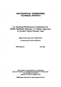
This paper builds on our previous efforts that have investigated the advantages of multiple cameras working in a non-stereo pair. Specifically, in [12,13], a new cooperative visual servoing approach was developed and experimentally demonstrated that using information from both an uncalibrated fixed camera and an uncalibrated on-board camera enables the on-board camera to track an object moving in the task-space with an unknown trajectory. A crucial assumption in [12,13] is that the camera and the object motion is constrained to a plane so that the unknown distance from the camera to the target remains constant. However, in contrast to [12,13], an on-board camera motion in this paper is not restricted to a plane. In our previous work [14], exponential regulation of an on-board camera is achieved despite uncertainty in the calibration parameters in contrast to asymptotic stability result in [15] by formulating a model-free rotation and composite translation controller. The proposed controller differs from [14,15] in the sense that the reference image need not be obtained using the same camera, i.e., it does not rely on the TBS paradigm. Further, TBZ control objective is formulated so that we can leverage the control development and stability analysis in [14] to achieve exponential regulation of an on-board camera in contrast to local asymptotic stability result proved in [5]. The developed controller is also invariant to the time-varying camera calibration parameters of a fixed camera since only constant parameter estimates are utilized in the control development, thus allowing the desired trajectory to be encoded using a stationary zooming-camera with e.g., time-varying focal length. Experimental results for regulation control of a 7 degrees-of-freedom (DOF) robotic manipulator are provided to demonstrate the performance of TBZ control. 2. Model development Consider the orthogonal coordinate systems F ; F f , and F  as depicted in Fig. 1. Coordinate system F is attached to an on-board camera (e.g., a camera held by a robot end-effector, a camera mounted on a vehicle) and F f is attached to a fixed camera that has an adjustable focal length to zoom in on an object. A captured image is defined by both the camera calibration parameters and the Euclidean position of the camera; therefore, the feature points of an object as seen in an image acquired by the fixed camera after zooming in on the object can be expressed in terms of F f in one of two ways: a different calibration matrix can be used due to the change in the focal length, or the calibration matrix can be held constant and the Euclidean position of the camera is changed to a virtual camera position and orientation. The position and orientation of the virtual camera is described by the coordinate system F  . A reference plane p is defined by four target points Oi "i = 1, 2, 3, 4 where the three dimensional (3D) coordinates of Oi expressed  i ðtÞ; m  fi and in terms of F ; F f , and F  are defined as elements of m  i 2 R3 as m

Fig. 1. Camera coordinate frame relationships, where frame F is attached to an onboard camera, F f is attached to a fixed camera, and F  represents a virtual camera.

438

S.S. Mehta et al. / Mechatronics 22 (2012) 436–443

 i ¼ ½ Xi m

Yi

Zi 

T T

 fi ¼ ½ X fi Y fi Z fi  m    i ¼ X fi Y fi Z i T : m

ð1Þ

The Euclidean-space is projected onto the image-space, so the  i ðtÞ; m  fi , and m  i normalized coordinates of the targets points m can be defined as

 i h Xi m ¼ Zi Zi  fi h X fi m mfi ¼ ¼ Zfi Z fi h   m X mi ¼ i ¼ Zfi i Zi mi ¼

Yi Zi

iT

1

Y fi Z fi Y fi Z i

1 1

iT

ð2Þ

iT

Assumption 1. The unknown target depth Z i ðtÞ; Z i , and Zfi > e, where e 2 R denotes a positive definite constant. It represents a standard assumption for vision-based systems that is consistent with the fact that a camera can view objects in front of the image plane. Based on (2) the normalized Euclidean coordinates of mfi can be related to  mi as 

Z i Z i ; ; 1 mi Z fi Z fi

mfi ¼ diag

ð3Þ

where diag {  } denotes a diagonal matrix of given arguments. In addition to having normalized task-space coordinates, each target point will also have pixel coordinates that are acquired from an on-board camera, expressed in terms of F , denoted by ui ðtÞ; v i ðtÞ 2 R, and are defined as elements of pi ðtÞ 2 R3 as

vi

pi , ½ ui

T

ð4Þ

1 :

The pixel coordinates pi(t) and the normalized task-space coordinates mi(t) are related by the following global invertible transformation (i.e., the pinhole model):

pi ¼ Ami :

ð5Þ

Constant pixel coordinates, expressed in terms of F f (denoted ufi ; v fi 2 R) and F  (denoted ui ; v i 2 R) are respectively defined as elements of pfi 2 R3 and pi 2 R3 as

pfi , ½ ufi

v fi

1

T

pi , ½ ui

v i

T

1 :

ð6Þ

The pinhole model can also be used to relate the pixel coordinates pfi and pi ðtÞ to the normalized task-space coordinates mfi and mi ðtÞ as

pfi ¼ Af mfi

ð7Þ

pi ¼ A mfi or pi ¼ Af mi :

ð8Þ

In (8), the first expression is where the Euclidean position and orientation of the camera remains constant and the camera calibration matrix changes, and the second expression is where the calibration matrix remains the same and the Euclidean position and orientation is changed. In (5) and (8), the intrinsic calibration matrices A, Af, and A 2 R33 denote the following constant invertible intrinsic camera calibration matrices:

3 k1 k1 cot / u0 60 k2 v 0 75 A,4 sin / 0 0 1 2 kf 1 kf 1 cot /f u0f 6 kf 2 Af , 6 v 0f 4 0 sin /

In (9), u0 ; v 0 2 R and u0f ; v 0f 2 R are the pixel coordinates of the principal point of an on-board camera and fixed camera, respectively. Constants k1 ; kf 1 ; k1 ; k2 ; kf 2 ; k2 2 R represent the product of camera scaling factors and focal length, and /, /f 2 R are the skew angles between the camera axes for an on-board camera and fixed camera, respectively. Since the intrinsic calibration matrix of a camera is difficult to accurately obtain, the development in this paper is based on the assumption that the intrinsic calibration matrices are unknown. Since Af is unknown, the normalized Euclidean coordinates mfi cannot be determined from pfi using Eq. (7). Since mfi cannot be determined, then the intrinsic calibration matrix A⁄ cannot be computed from (8). For the TBZ problem formulation, pi defines the desired image-space coordinates. Since the normalized Euclidean coordinates mi are unknown, the control objective is defined in terms of servoing an on-board camera so that the images correspond. If the image from an on-board camera and the zoomed image from a fixed camera correspond, then the following expression can be developed from (5) and (8):

mi ¼ mdi , A1 Af mi

ð10Þ

3

where mdi 2 R denotes the normalized Euclidean coordinates of the object feature points expressed in F d . F d denotes the coordinate system attached to an on-board camera when the image taken from an on-board camera corresponds to the image acquired from a fixed camera after zooming in on an object. Hence, the control objective for uncalibrated TBZ problem can be formulated as the desire to force mi(t) to mdi. Given that mi ðtÞ; mi , and mdi are unknown, the ^ i ðtÞ; m ^ i , and m ^ di 2 R3 are defined to facilitate the subseestimates m quent control development [15]

b 1 p ¼ Am e i ^i ¼ A m i  1  b p ¼A e f m ^ ¼A m

ð11Þ

b 1 p A i

ð13Þ

i

^ di ¼ m

f

i

ð12Þ

i

e di ¼ Am

b A b f 2 R33 are constant, best-guess estimates of the intrinwhere A; sic camera calibration matrices1 A and Af, respectively. The calibrae A e f 2 R33 are defined as tion error matrices A;

2

e 11 A 6 1 e b A,A A¼4 0 0 2e A f 11 ef , A b 1 Af ¼ 6 A 4 0 f 0

3 e 13 A e 23 7 5 A

e 12 A e A 22 0

ð14Þ

1

e f 12 A e f 22 A 0

e f 13 3 A e f 23 7 5: A

ð15Þ

1

Remark 1. For the standard TBS visual servo control problem where the camera calibration parameters do not change between the teaching phase and the servo phase, i.e., A = Af, the coordinate frames F d and F  are identical.

2

f

2

0 k1

6 A , 6 40 0

0 k1 cot /f k2 sin /f

0

1 u0f

3. Homography development

7 7 5

ð9Þ

 i þ xf  i ¼ Rm m

ð16Þ

3 7

v 0f 75: 1

The following expression can be obtained based on the relationship between coordinate frames F and F  (see Fig. 1):

3

1 b and A b can be obtained by approximate camera calibration or by The estimates A f referring to the manufacturer specifications.

439

S.S. Mehta et al. / Mechatronics 22 (2012) 436–443

where RðtÞ 2 R33 and xf ðtÞ 2 R3 denote the rotation and translation, respectively, between F and F  . By utilizing (1) and (2), the expression in (16) can be expressed as

mi ¼

  Zi T ðR þ xh n Þ m Z i |fflfflfflfflfflfflfflffl{zfflfflfflfflfflfflfflffl} i |fflffl{zfflffl} H

ð17Þ

ai

x ðtÞ



where xh ðtÞ , fd 2 R3 and d 2 R denotes an unknown constant distance from F  to p along the unit normal n⁄. The following relationship can be developed by substituting (17) and (8) into (5) for mi(t) and mi , respectively:  i Gpi

pi ¼ a

ð18Þ 33

where G 2 R is the projective homography matrix defined as GðtÞ , AHðtÞA1 f . The expressions in (5) and (8) can be used to rewrite (18) as

mi ¼ ai A1 GAf mi :

ð19Þ

The following expression can be obtained by substituting (10) into (19):

mi ¼ ai Hd mdi

ð20Þ 1

where Hd(t) , A G(t)A denotes the Euclidean homography matrix that can be expressed as

Hd ¼ Rd þ xhd nTd

where xhd ¼

xfd : dd

ð21Þ

In (21), Rd ðtÞ 2 R33 and xfd ðtÞ 2 R3 denote the rotation and translation, respectively, from F to F d . The constant dd 2 R in (21) denotes the distance from F d to p along the unit normal nd 2 R3 . Since mi(t) and mi cannot be determined because the intrinsic camera calibra^ i ðtÞ and m ^ di detion matrices and Af are uncertain, the estimates m fined in (11) and (12), respectively, can be utilized to obtain the following:

b dm ^ i ¼ ai H ^ di : m

ð22Þ

b d ðtÞ 2 R33 denotes the following estimated Euclidean In (22), H homography [15]:

The control objective is to ensure that the position and orientation of the camera coordinate frame F is regulated to F d . Based on Section 3, the control objective is achieved if

Rd ðtÞ ! I3

ð29Þ

and one target point is regulated to its desired location in the sense that

mi ðtÞ ! mdi and Z i ðtÞ ! Z di :

ð30Þ

To control the position and orientation of F , a relationship is required to relate the linear and angular camera velocities to the linear and angular velocities of the vehicle/robot (i.e., the actual kinematic control inputs) that enables an on-board camera motion. This relationship is dependent on the extrinsic calibration parameters as [15]



vc

xc

¼

Rr

½ t r   Rr

0

Rr



vr

ð31Þ

xr

where v c ðtÞ; xc ðtÞ 2 R3 denote the linear and angular velocity of the camera, v r ðtÞ; xr ðtÞ 2 R3 denote the linear and angular velocity of the vehicle/robot, Rr 2 R33 denotes the unknown constant rotation between an on-board camera and robot end-effector frames, and ½t r  2 R33 is a skew symmetric form of t r 2 R3 , which denotes the unknown constant translation vector between an on-board camera and vehicle/robot frames.

ð23Þ

^ i ðtÞ and m ^ di can be determined from (11) and (13), a set of Since m b d ðtÞ (see [16] for linear equations can be developed to solve for H additional details regarding the set of linear equations). The expression in (23) can also be expressed as [16]

b d þ ^xhd n bd ¼ R ^ Td : H

ð24Þ

b d ðtÞ 2 R33 , is reIn (24), the estimated rotation matrix, denoted R lated to Rd(t) as below

e dA e 1 ; b d ¼ AR R

ð25Þ ^ Td n

3

and ^xhd ðtÞ 2 R ; 2 R denote the estimate of xhd(t) and nd, respectively, and are defined as

e hd ^xhd ¼ c Ax 1 e T ^d ¼ A nd n

c

ð26Þ ð27Þ

5.1. Rotation controller To quantify the rotation between F and F d (i.e., Rd(t) given in (21)), a rotation error-like signal, denoted by ex ðtÞ 2 R3 , is defined by the angle axis representation as

ex ¼ uh

ð32Þ 3

where uðtÞ 2 R represents a unit rotation axis, and hðtÞ 2 R denotes the rotation angle about u(t) that is assumed to be constrained to the region

0 6 hðtÞ 6 p:

ð33Þ

The parameterization u(t)h(t) is related to the rotation matrix Rd(t) as 2

Rd ¼ I3 þ sin h½u þ 2 sin

h 2 ½u 2 

ð34Þ

where [u] denotes the 3  3 skew-symmetric matrix associated with u(t). The open-loop error dynamics for ex(t) can be expressed as

where c 2 R denotes the following positive constant

c ¼ k Ae T nd k:

4. Control objective

5. Control development

e 1 : e dA b d ¼ AH H

3

To address this issue, additional information (e.g., at least four vanishing points) can be used. For example, as the reference plane p approaches infinity, the scaling term d⁄ also approaches infinity, and xh ðtÞ; ^ xh ðtÞ approach zero. Hence, (24) can be used to conclude b d ðtÞ ¼ R b d ðtÞ on the plane at infinity, and the four vanishing that H b d ðtÞ. Once point pairs can be used along with (22) to determine R b R d ðtÞ has been determined, various techniques (e.g., see [17,19]) can be used along with the original four image point pairs to deter^ d ðtÞ. mine ^ xhd ðtÞ and n

ð28Þ

b d ðtÞ can be computed, standard techniques cannot Although H b d ðtÞ into the rotation and translation combe used to decompose H b d ðtÞ is not a true rotation ponents in (24). Specifically, from (25) R matrix, and hence, it is not clear how standard decomposition algorithms (e.g., the Faugeras algorithm [17,18]) can be applied.

e_ x ¼ Lx Rr xr

ð35Þ 33

where Lx ðtÞ 2 R

is defined as

! h sincðhÞ ½u2 : Lx ¼ I3  ½u þ 1  2 2 sinc h 2

ð36Þ

440

S.S. Mehta et al. / Mechatronics 22 (2012) 436–443

where me ðtÞ 2 R3 denotes the extended coordinates of an image point on p expressed in terms of F and is defined as2

In Eq. (36) the sinc (h) term is given by (37) as,

sincðhÞ ¼

sinðhÞ h

ð37Þ

Since the rotation matrix Rd(t) and the rotation error ex(t) defined in (32) are unmeasurable, an estimated rotation error ^ex ðtÞ 2 R3 is defined as

^ ^h ^ex ¼ u

ð38Þ

^ ðtÞ 2 R3 ; ^ where u hðtÞ 2 R represent estimates of u(t) and h(t), b d ðtÞ is similar to Rd(t) (i.e., R b d ðtÞ has the same respectively. Since R ^ ðtÞ and ^ trace and eigenvalues as Rd(t)), the estimates u hðtÞ can be related to u(t) and h(t) as [15]

e ^h ¼ h u ^ ¼ l Au where

ð39Þ

lðtÞ 2 R denotes the following unknown function 1

l¼ e : k Auk

ð40Þ

The relationship in (39) allows ^ex ðtÞ to be expressed in terms of the unmeasurable error ex(t) as

e x: ^ex ¼ l Ae

ð41Þ

Given the open-loop rotation error dynamics in (35), the control input xr(t) is designed as

xr ¼ kx Rb Tr ^ex

ð42Þ

b r 2 R33 denotes where kx 2 R denotes a positive control gain, and R a constant best-guess estimate of Rr. Substituting (41) into (42) and substituting the resulting expression into (35) gives the following expression for the closed-loop error dynamics [15]:

e x e r Ae e_ x ¼ kx lLx R

ð43Þ

e r 2 R33 is defined as where the extrinsic rotation estimation error R

e r ¼ Rr R bT : R r

me , ½ me1 ðtÞ me2 ðtÞ me3 ðtÞ T ¼

mde , ½ mde1

ð45Þ

provided the following inequality is satisfied:

e P b kxk2 for 8x 2 R3 e r AÞx xT ð R 0

ð46Þ

where

x

T

! 

T e e e e T T e e T R r A þ ð R r AÞ e e Rr A x ¼ x Rr A x ¼ x x 2

ð47Þ

for 8x 2 R3 ; and b0 2 R denotes the minimum eigenvalue as below

(

b0 ¼ kmin

) e þ ðR e T er A e r AÞ R : 2

ð48Þ

ev ¼

h

X1 Z1

ev , me  mde

ð49Þ

2 To develop the translation controller a single feature point can be utilized. Without loss of generality, the subsequent development will be based on the image point O1, and hence, the subscript 1 will be utilized in lieu of i.

lnðZ 1 Þ

iT

ð50Þ

h

mde3 T ¼

X d1 Z 1

Y d1 Z 1

 iT ln Z 1

ð51Þ

1

Y1 Z1

 YZd1

ln

1

 iT Z1 Z 1

ð52Þ

where the ratio ZZ1 can be computed from (17) and the decomposi1 tion of the estimated Euclidean homography in (22). Since m1(t) and md are unknown (since the intrinsic calibration matrices are unknown), ev(t) is not measurable. Therefore, the estimate of the translation error system given in (52) is defined as

h ^ e1  m ^ de1 ^ev , m

^ de2 ^ e2  m m

ln

 iT Z1 Z 1

ð53Þ

^ e1 ðtÞ; m ^ e2 ðtÞ; m ^ de1 ; m ^ de2 2 R denote estimates of me1(t), where m me2(t), mde1, mde2, respectively. To develop the closed-loop error system for ev(t), we take the time derivative of (52) and then substitute (42) into the resulting expression for xr(t) to obtain

e r ^ex e_ v ¼ Lv Rr v r þ kw ðLv ½t r  þ Lv x Þ R 3x3

where Lv ðtÞ; Lv x ðtÞ 2 R

2

Lv ,

ð54Þ

are defined as

3

1 0 me1 16 7 4 0 1 me2 5 Z1 0 0 1 me1 me2

6 Lv x , 4 1 þ m2e2 me2

1  m2e1 me1 me2 me1

ð55Þ

me2

3

7 me1 5:

ð56Þ

0

To facilitate the control development, the unknown depth Z1(t) in (55) can be expressed as

Z1 ¼

1

a1

Z 1

ð57Þ

where a1 is given by the homography decomposition. An estimate for Lv(t) can be designed as

2 3 ^ e1 1 0 m 1 6 b ^ e2 7 Lv ¼ 4 0 1 m 5; b1 Z 0 0 1

ð58Þ

b 1 ðtÞ 2 R is devel^ e1 ðtÞ; m ^ e2 ðtÞ were introduced in (53), and Z where m oped based on (57) as

a1

The difference between the actual and desired 3D Euclidean camera position, denoted by the translation error signal ev ðtÞ 2 R3 , is defined as

mde2

 XZd1

b1 ¼ 1 Z b : Z 1

5.2. Translation controller

Y1 Z1

where ln () denotes the natural logarithm. Substituting (50) and (51) into (49) yields

2

kex ðtÞk 6 kex ð0Þk expðkx lb0 tÞ

X1 Z1

and mde 2 R3 denotes the extended coordinates of the corresponding desired image point on p in terms of F d as

ð44Þ

Property 1. The kinematic control input given in (42) ensures that ex(t) defined in (32) is exponentially regulated in the sense that [14]

h

ð59Þ

b  is an estimate of the constant unknown Remark 2. In (59), Z 1  depth Z 1 and is assumed to be known with an uncertainty. However, the constant parameter Z 1 can also be estimated online in a direct adaptive framework [16].

Based on the structure of an error system in (54) and subsequent stability analysis, the following composite translation controller can be developed

441

S.S. Mehta et al. / Mechatronics 22 (2012) 436–443

ω1 [deg/s]

Fig. 2. (A) Robotics Research K-1607 manipulator in a camera-in-hand configuration; (B) initial and (C) final position of the feature points as viewed by the camera-in-hand (green points) and the overlaid desired feature points captured by the fixed camera (red points). (For interpretation of the references to colour in this figure legend, the reader is referred to the web version of this article.)

[deg]

100

e

ω1

50 0 −50

0

20

40

60

80

100

250 0 −250 −500

0

20

40

time [s]

ω2 [deg/s]

[deg]

100 50

e

ω2

0 −50

0

20

40

60

80

100

−50 40 time [s]

60

80

100

−500

0

20

40

eν1

80

100

60

80

100

250 0 −250 −500

0

20

40

Fig. 5. Rotation velocity control input about x-axis (x1(t)), y-axis (x2(t)), and z-axis (x3(t)) of the camera coordinate frame.

b 1 ðtÞ is defined in (59). In (60), kv ðtÞ 2 R denotes a positive gain and Z function defined as

0.5 0 0

20

40

60

80

100

kv ¼ kn0 þ

time [s]

b2 Z 1 ^ e1 ; m ^ e2 Þ f ðm

ð61Þ

^ e1 ; m ^ e2 Þ is a positive where kn0 2 R is a positive constant, and f ðm ^ e1 and m ^ e2 . function of m

0.5

eν2

60

0 −250

time [s]

Fig. 3. Rotation error plot indicating angular error about x-axis (ex1(t)), y-axis (ex2(t)), and z-axis (ex3(t)) of the camera coordinate frame.

−0.5

ω3 [deg/s]

eω3 [deg]

0

20

100

time [s]

50

0

80

250

time [s]

−100

60

time [s]

0 −0.5

0

20

40

60

80

100

time [s]

Property 2. The kinematic control input given in (60) ensures that the composite translation error signal ev(t) defined in (52) is exponentially regulated in the sense that [14]

eν3

1

kev ðtÞk 6

0 −1

0

20

40

60

80

100

time [s] Fig. 4. Linear error plot indicating discrepancy between the extended normalized Euclidean coordinates of the target between the current and desired configurations.

v r ðtÞ ¼ kv Rb Tr bL Tv ^ev 

 T^ b 2 þ kn2 Z b 2 k^ev k2 R bT b kn1 Z 1 1 r L v ev

ð60Þ

b T ; ^ev ðtÞ, and b where R L v ðtÞ are introduced in (42), (53), and (58), r respectively, kn1 ; kn2 2 R denote positive constant control gains,

  pffiffiffiffiffiffiffi 1 f 2f0 kB k exp  1 t 2

ð62Þ

provided (46) is satisfied, where B 2 R3x3 is a constant invertible matrix, and f0 ; f1 2 R denote positive constants. 6. Experimental results An experiment was performed using a Robotics Research K1607 7-DOF robotic manipulator, as shown in Fig. 2A, to demonstrate the performance of the TBZ controller given in (42) and (60). The robot end-effector was equipped with a SONY CCD block camera and a mvBlueFox CCD camera fitted with a variable focal length lens served as a fixed camera. Location of the camera-in-

442

S.S. Mehta et al. / Mechatronics 22 (2012) 436–443

the camera-in-hand and end-effector frame, i.e., the extrinsic camb r and ^tr defined in (31), are measured era calibration parameters R to be

ν1 [in/s]

200 0 −200

0

20

40

60

80

100

ν2 [in/s]

time [s] 200 0

−200

0

20

40

60

80

100

60

80

100

ν3 [in/s]

time [s] 1000 500 0 −500

0

20

40

time [s] Fig. 6. Linear velocity control input along x-axis (v1(t)), y-axis (v2(t)), and z-axis (v3(t)) of the camera coordinate frame.

e (t) [pixel] p1

400 200 0 −200 −400

3 1 0 0 6 b r ¼ 4 0 0:9974 0:0724 7 R 5; 0 0:0724 0:9974

ð63Þ

^t r ¼ ½ 100:3 48:0 48:0 T :

ð64Þ

b r and ^tr are obtained using the commercial grade The estimates R digital level and laser range finder, respectively, within the accuracy of the sensors. Since the z-axis of camera frame F is parallel to the x-axis of robot end-effector frame there exists a rotation Rx(n) about the x-axis of end-effector frame by an angle n 2 R that will align camera frame to the end-effector frame. The extrinsic calibration b r 2 R33 in (63) is then obtained as Rx(n) by measuring matrix R the constant angle n. The translation estimate ^t r given in (64) is obtained by measuring the components of position vector corresponding to the origin of the camera coordinate frame F in the end-effector frame using a laser range finder. The control objective is to regulate the camera-in-hand to the position/orientation of the virtual camera coordinate frame representing the zoomed in position/orientation of the fixed camera. The control gains kn0, kn1, kn2, and kw were adjusted to the following values to yield the best performance

kn0 ¼ 40 kn1 ¼ 26:6 kn2 ¼ 26:6 kw ¼ 6:0: 0

20

40

60

80

100

60

80

100

time [s]

ep2(t) [pixel]

2

200 100 0 0

20

40

time [s] Fig. 7. Image space error ep(t) showing the difference in pixel coordinates between the current and reference images along the image x- and y-axes.

hand and fixed camera was selected such that a set of four coplanar features can be viewed by both the cameras. The focal length of the fixed camera was varied (zoomed in) to obtain the feature points pi corresponding to the desired position/orientation, while a pyramidal implementation of the Lucas Kanade (KLT) feature tracker provided the time-varying feature points pi(t) for the camera-in-hand. In an event where the camera-in-hand can be located a priori to the desired position/orientation of a robotic manipulator, the feature points pi as well as pi(t) are obtained by the camera-in-hand and the TBZ control law presented in (42) and (60) becomes identical to TBS controller. Caltech camera calibration toolbox for Matlab was used to obtain the estimates of intrinsic calibration parameters for both the cameras. The principal point image coordinates for the camera-in-hand and fixed camera are considered to be u0 = 345, v0 = 245 and u0f = 302, v0f = 272, respectively; k1 ¼ 868; k2 ¼ 878; kf 1 ¼ 571; kf 2 ¼ 571; k1 ¼ 1596; k2 ¼ 1597 denote the product of focal length and scaling factors for an on-board camera, fixed camera, and fixed camera after zooming, respectively; and / = /f = 1.53 (rad) is the skew angle for each camera. The intrinsic parameters k1 and k2 , corresponding to the zoomed-in position of the lens, were computed to evaluate the correctness of servo control and were not used in the control formulation. The constant rotation and translation between

ð65Þ

The feature points viewed by the camera-in-hand before and at the end of the servo control are shown in Figs. 2B and 2C, respectively, along with the location of desired feature points captured by the fixed camera. The resulting rotation and unitless translation errors are depicted in Figs. 3 and 4, respectively. The angular and linear control input velocities xr(t) and tr(t) defined in (42) and (60), respectively, are shown in Figs. 5 and 6. It can be observed from Figs. 3 and 4 that the rotation and translation error between camera coordinate frames F and F  vanishes exponentially, thus regulating the camera-in-hand to the position/orientation of the virtual camera coordinate frame representing the zoomed in position/orientation of the fixed camera; Figs. 5 and 6 show that the linear and angular velocity control inputs remain bounded during the closed-loop operation. The image-space error ep ðtÞ 2 R3 between the desired and current image coordinates of the target point O1 is defined as

ep ðtÞ ¼ ½ ep1

ep2

ep3 T ¼ p1 ðtÞ  p1 :

ð66Þ

Fig. 7 shows the plot of the image error ep(t) defined in (66) to demonstrate the regulation result in an image-space. 7. Conclusion A unified visual servo control approach – teach by zooming – is presented to address the control problem in applications where the camera cannot be a priori positioned to the desired position/orientation to acquire a reference image. Specifically, the TBZ control objective is formulated to position/orient an on-board camera based on a reference image obtained by another camera. In addition to formulating the TBZ control problem, another contribution of this paper is to illustrate how to preserve a symmetric transformation from the projective homography to the Euclidean homography for problems when the corresponding images are taken from different cameras with calibration uncertainty. To this end, a desired camera position/orientation is defined where the images correspond, but the Euclidean position differs as a function of the mismatch in the calibration of the cameras. Applications of this

S.S. Mehta et al. / Mechatronics 22 (2012) 436–443

strategy could include navigating ground or air vehicles based on the desired images taken by other ground or air vehicles (e.g., a satellite captures a ‘‘zoomed in desired image that is used to navigate an unmanned aerial vehicle (UAV), a camera can view the entire tree canopy and zoom in to acquire a desired image of a fruit product for high speed robotic harvesting). Experimental results are provided to demonstrate the performance of the developed controller.

References [1] Corke P. Visual control of robot manipulators – a review. World scientific series in robotics and automated systems, vol. 7. World Scientific Press; 1993. [2] Hashimoto K. A review on vision-based control of robot manipulators. Adv Robot 2003;17(10):969–91. [3] Malis E, Chaumette F, Bodel S. 2-1/2D visual servoing. IEEE Trans Robot Automat 1999;15(2):238–50. [4] Hutchinson S, Hager G, Corke P. A tutorial on visual servo control. IEEE Trans Robot Automat 1996;12(5):651–70. [5] Malis E. Visual servoing invariant to changes in camera-intrinsic parameters. IEEE Trans Robot Automat 2004;20(1):72–81. [6] Malis M. Vision-based control using different cameras for learning the reference image and for servoing. In: Proceedings of the IEEE/RSJ international conference on intelligent robots and systems, vol. 3; 2001. p. 1428–33. [7] Dixon W. Teach by zooming: a camera independent alternative to teach by showing visual servo control. In: Proceedings of the IEEE/RSJ international conference on intelligent robots and systems, vol. 1; 2003. p. 749–54.

443

[8] Mehta S, Dixon W, Burks T, Gupta S. Teach by zooming visual servo control for an uncalibrated camera system. In: Proceedings of the AIAA guidance, navigation and control conference and exhibit; 2005. p. AIAA–2005–6095. [9] Espiau B. Effect of camera calibration errors on visual servoing in robotics. In: 3rd International symposium on experimental robotics; 1993. p. 187–93. [10] Chaumette F, Hutchinson S. Visual servo control: i – basic approaches. IEEE Robot Automat Mag 2006;13(4):82–90. [11] Chaumette F. Potential problems of stability and convergence in image-based and position-based visual servoing. In: Kriegman D, Hager G, Morse A, editors. The confluence of vision and control. Lecture notes in control and information sciences, vol. 237. Berlin/Heidelberg: Springer; 1998. p. 66–78. [12] Dixon W, Love L. Lyapunov-based visual servo control for robotic deactivation and decommissioning. In: The 9th biennial ANS international spectrum conference; 2002. [13] Dixon W, Zergeroglu E, Fang Y, Dawson D. Object tracking by a robot manipulator: a robust cooperative visual servoing approach. In: Proceedings of the IEEE international conference on robotics and automation, vol. 1; 2002. p. 211–6. [14] Fang Y, Dixon W, Dawson D, Chen J. An exponential class of model-free visual servoing controllers in the presence of uncertain camera calibration. Int J Robot Automat 2006;21(4):247–55. [15] Malis E, Chaumette F. Theoretical improvements in the stability analysis of a new class of model-free visual servoing methods. IEEE Trans Robot Automat 2002;18(2):176–86. [16] Fang Y, Behal A, Dixon W, Dawson D. Adaptive 2.5D visual servoing of kinematically redundant robot manipulators. In: Proceedings of the 41st IEEE conference on decision and control, vol. 3; 2002. p. 2860–5. [17] Faugeras O, Lustman F. Motion and structure from motion in a piecewise planar environment. Int J Pattern Recogn Artif Int 1988;2(3):485–508. [18] Faugeras O. The geometry of multiple images. MIT Press; 2001. [19] Zhang Z, Hanson A. Scaled euclidean 3D reconstruction based on externally uncalibrated cameras. In: Proceedings of the international symposium on computer vision; 1995. p. 37–42.