Barbalat's Lemma [62] can then be used to prove the result given in (33). Based on the controller in (26) and (27) and the adaptive law in (28), the resulting ...
1
Adaptive Visual Servo Control G. Hu, N. Gans, and W. E. Dixon Department of Mechanical and Aerospace Engineering, University of Florida, Gainesville, Florida
C ONTENTS I
Glossary
2
II
Definition of the Subject and Its Importance
3
III
Introduction
3
IV
Visual Servo Control Methods IV-A Geometric Relationships . . . . . . . . . IV-B Image-based Visual Servo Control . . . . IV-C Position-Based Visual Servo Control . . . IV-D Homography-Based Visual Servo Control IV-E Simulation Comparisons . . . . . . . . .
V
VI
VII
. . . . .
. . . . .
. . . . .
. . . . .
. . . . .
. . . . .
. . . . .
. . . . .
. . . . .
. . . . .
5 5 7 8 9 9
Compensating for Projection Normalization V-A Adaptive Depth Compensation in Homography-Based Visual Servo Control V-A.1 Open-Loop Error System . . . . . . . . . . . . . . . . . . . . . . V-A.2 Controller and Adaptive Law Design . . . . . . . . . . . . . . . V-A.3 Closed-Loop Stability Analysis . . . . . . . . . . . . . . . . . . . V-B Adaptive Depth Compensation in Image-Based Visual Servo Control . . . . V-B.1 Open-Loop Error System . . . . . . . . . . . . . . . . . . . . . . V-B.2 Controller and Adaptive Law Design . . . . . . . . . . . . . . . V-B.3 Closed-Loop Stability Analysis . . . . . . . . . . . . . . . . . . .
. . . . . . . .
. . . . . . . .
. . . . . . . .
. . . . . . . .
. . . . . . . .
. . . . . . . .
. . . . . . . .
. . . . . . . .
. . . . . . . .
10 10 11 11 11 12 12 14 15
Visual Servo Control via an Uncalibrated Camera VI-A Jacobian Estimation Approach . . . . . . . . . . . . . . . . . . . . VI-B Robust Control Approach . . . . . . . . . . . . . . . . . . . . . . . VI-B.1 State Estimation . . . . . . . . . . . . . . . . . . . . . . VI-B.2 Control Development and Stability Analysis . . . . . . . VI-C Adaptive Image-Based Visual Servo Control Approach . . . . . . . VI-C.1 Open-Loop Error System . . . . . . . . . . . . . . . . . VI-C.2 Controller and Adaptive Law Design . . . . . . . . . . VI-D Adaptive Homography-Based Visual Servo Control Approach . . . VI-D.1 Problem Statement and Assumptions . . . . . . . . . . . VI-D.2 Euclidean Reconstruction Using Vanishing Points . . . . VI-D.3 Open-Loop Error System . . . . . . . . . . . . . . . . . VI-D.4 Rotation Controller Development and Stability Analysis VI-D.5 Translation Control Development and Stability Analysis
. . . . . . . . . . . . .
. . . . . . . . . . . . .
. . . . . . . . . . . . .
. . . . . . . . . . . . .
. . . . . . . . . . . . .
. . . . . . . . . . . . .
. . . . . . . . . . . . .
. . . . . . . . . . . . .
. . . . . . . . . . . . .
15 16 16 16 17 18 19 20 21 21 21 22 23 24
Future Directions
References
. . . . .
. . . . .
. . . . .
. . . . .
. . . . .
. . . . .
. . . . .
. . . . .
. . . . .
. . . . .
. . . . .
. . . . .
. . . . .
. . . . .
. . . . .
. . . . . . . . . . . . .
. . . . .
. . . . . . . . . . . . .
. . . . .
. . . . . . . . . . . . .
. . . . .
. . . . . . . . . . . . .
. . . . . . . . . . . . .
25 27
2
I. G LOSSARY Camera-in-hand configuration The camera-in-hand configuration refers to the case when the camera is attached to a moving robotic system (e.g., held by the robot end-effector). Camera-to-hand configuration The camera-to-hand configuration refers to the case when the camera is stationary and observing moving targets (e.g., a fixed camera observing a moving robot end-effector). Euclidean Reconstruction Euclidean reconstruction is the act of reconstructing the Euclidean coordinates of feature points based on the two-dimensional image information obtained from a visual sensor. Extrinsic calibration parameters The extrinsic calibration parameters are defined as the relative position and orientation of the camera reference frame to the world reference frame (e.g., the frame affixed to the robot base). The parameters are represented by a rotation matrix and a translation vector. Feature point Different computer vision algorithms have been developed to search images for distinguishing features in an image (e.g., lines, points, corners, textures). The three-dimensional Euclidean-space representation of a point in the two-dimensional image-plane is called a feature point. Feature points are selected based on contrast with surrounding pixels and the ability for the point to be tracked from frame to frame. Sharp corners (e.g., the windows of a building), or center of a homogenous region in the image (e.g., the center of car headlights) are typical examples of feature points. Homography The geometric concept of homography is a one-to-one and on-to transformation or mapping between two sets of points. In computer vision, homography refers to the mapping between points in two Euclidean-planes (Euclidean homography), or to the mapping between points in two images (projective homography). Image Jacobian The image-Jacobian is also called the interaction matrix, feature sensitivity matrix, or feature Jacobian. It is a transformation matrix that relates the change of the pixel coordinates of the feature points on the image to the velocity of the camera. Intrinsic calibration parameters The intrinsic calibration parameters map the coordinates from the normalized Euclidean-space to the imagespace. For the pinhole camera, this invertible mapping includes the image center, camera scale factors, and camera magnification factor. Pose The position and orientation of an object is referred to as the pose. The pose has a translation component that is an element of R3 (i.e., Euclidean-space), and the rotation component is an element of the special orthogonal group SO(3), though local mappings of rotation that exist in R3 (Euler angles, angle/axis) or R4 (unit quaternions). Pose of an object has specific meaning when describing the relative position and orientation of one object to another or the position and orientation of an object at different time instances. Pose is typically used to describe the position and orientation of one reference frame with respect to another frame. Projection Normalization The Euclidean coordinates of a point are projected onto a two-dimensional image via the projection normalization. For a given camera, a linear projective matrix can be used to connect pixel coordinates on the image-plane to the corresponding points in the Euclidean-space. This relationship is not bijective because there exist infinite number of Euclidean points that have the same normalized coordinates, and the depth information is lost during the normalization. Unit Quaternion The quaternion is a four dimensional vector which is composed of real numbers (i.e., q ∈ R4 ). The unit quaternion is a quaternion subject to a nonlinear constraint that the norm is equal to 1. The unit quaternion can be used as a globally nonsingular representation of a rotation matrix. Visual Servo Control System
3
Control systems that use information acquired from an imaging source (e.g., a digital camera) in the feedback control loop are defined as visual servo control systems. In addition to providing feedback relating the local position and orientation (i.e., pose) of the camera with respect to some target, an image sensor can also be used to relate local sensor information to an inertial reference frame for global control tasks. Visual servoing requires multidisciplinary expertise to integrate a vision system with the controller for tasks including: selecting the proper imaging hardware; extracting and processing images at rates amenable to closed-loop control; image analysis and feature point extraction/tracking; recovering/estimating necessary state information from an image; and operating within the limits of the sensor range (i.e., field-of-view). Lyapunov Function A Lyapunov function is a continuously differentiable positive definite function with a negative semi-definite time-derivative. II. D EFINITION OF THE S UBJECT AND I TS I MPORTANCE Control systems that use information acquired from an imaging source in the feedback loop are defined as visual servo control systems. Visual servo control has developed into a large subset of robotics literature because of the enabling capabilities it can provide for autonomy. The use of an image sensor for feedback is motivated by autonomous task execution in an unstructured or unknown environments. In addition to providing feedback relating the local position and orientation (i.e., pose) of the camera with respect to some target, an image sensor can also be used to relate local sensor information to an inertial reference frame for global control tasks. However, the use of image-based feedback adds complexity and new challenges for the control system design. Beyond expertise in design of mechanical control systems, visual servoing requires multidisciplinary expertise to integrate a vision system with the controller for tasks including: selecting the proper imaging hardware; extracting and processing images at rates amenable to closed-loop control; image analysis and feature point extraction/tracking; recovering/estimating necessary state information from an image; and operating within the limits of the sensor range (i.e., field-of-view). While each of the aforementioned tasks are active topics of research interest, the scope of this chapter is focused on issues associated with using reconstructed and estimated state information from an image to develop a stable closed-loop error system. That is, the topics in this chapter are based on the assumption that images can be acquired, analyzed, and the resulting data can be provided to the controller without restricting the control rates. III. I NTRODUCTION The different visual servo control methods can be divided into three main categories including: image-based, position-based, and approaches that use of blend of image and position-based approaches. Image-based visual servo control (e.g., [1]–[5]) consists of a feedback signal that is composed of pure image-space information (i.e., the control objective is defined in terms of an image pixel error). This approach is considered to be more robust to camera calibration and robot kinematic errors and is more likely to keep the relevant image features in the fieldof-view than position-based methods because the feedback is directly obtained from the image without the need to transfer the image-space measurement to another space. A drawback of image-based visual servo control is that since the controller is implemented in the robot joint space, an image-Jacobian is required to relate the derivative of the image-space measurements to the camera’s linear and angular velocities. However, the image-Jacobian typically contains singularities and local minima [6], and the controller stability analysis is difficult to obtain in the presence of calibration uncertainty [7]. Another drawback of image-based methods are that since the controller is based on image-feedback, the robot could be commanded to some configuration that is not physically possible. This issue is described as Chaumette’s conundrum (see [6], [8]). Position-based visual servo control (e.g., [1], [5], [9]–[11]) uses reconstructed Euclidean information in the feedback loop. For this approach, the image-Jacobian singularity and local minima problems are avoided, and physically realizable trajectories are generated. However, the approach is susceptible to inaccuracies in the taskspace reconstruction if the transformation is corrupted (e.g., uncertain camera calibration). Also, since the controller does not directly use the image features in the feedback, the commanded robot trajectory may cause the feature points to leave the field-of-view. A review of these two approaches is provided in [5], [12], [13]. The third class of visual servo controllers use some image-space information combined with some reconstructed information as a means to combine the advantages of these two approaches while avoiding their disadvantages
4
(e.g., [8], [14]–[23]). One particular approach was coined 2.5D visual servo control in [15]–[18] because this class of controllers exploits some two dimensional image feedback and reconstructed three-dimensional feedback. This class of controllers is also called homography-based visual servo control in [19]–[22] because of the underlying reliance of the construction and decomposition of a homography. A key issue that is pervasive to all visual servo control methods is that the image-space is a two-dimensional projection of the three-dimensional Euclidean-space. To compensate for the lack of depth information from the twodimensional image data, some control methods exploit additional sensors (e.g., laser and sound ranging technologies) along with sensor fusion methods or the use of additional cameras in a stereo configuration that triangulate on corresponding images. However, the practical drawbacks of incorporating additional sensors include: increased cost, increased complexity, decreased reliability, and increased processing burden. Geometric knowledge of the target or scene can be used to estimate depth, but this information is not available for many unstructured tasks. Motivated by these practical constraints, direct approximation and estimation techniques (cf. [4], [5]) and dynamic adaptive compensation (cf. [19]–[22], [24]–[28]) have been developed. For example, an adaptive kinematic controller has been developed in [24] to achieve a uniformly ultimately bounded regulation control objective provided conditions on the translation velocity and bounds on the uncertain depth parameters are satisfied. In [24], a three dimensional depth estimation procedure has been developed that exploits a prediction error provided a positive definite condition on the interaction matrix is satisfied. In [20], [26], [27], homography-based visual servo controllers have been developed to asymptotically regulate a manipulator end-effector and a mobile robot, respectively, by developing an adaptive update law that actively compensates for an unknown depth parameter. In [19], [21], adaptive homography-based visual servo controllers have been developed to achieve asymptotic tracking control of a manipulator end-effector and a mobile robot, respectively. In [22], [28], adaptive homography-based visual servo controllers via a quaternion formulation have been developed to achieve asymptotic regulation and tracking control of a manipulator end-effector, respectively. In addition to normalizing the three-dimensional coordinates, the projection from the Euclidean-space to the image-space also involves a transformation matrix that may contain uncertainties. Specifically, a camera model (e.g., the pinhole model) is often required to relate pixel coordinates from an image to the (normalized) Euclidean coordinates. The camera model is typically assumed to be exactly known (i.e., the intrinsic calibration parameters are assumed to be known); however, despite the availability of several popular calibration methods (cf. [29]–[35]), camera calibration can be time consuming, requires some level of expertise, and has inherent inaccuracies. If the calibration parameters are not exactly known, performance degradation and potential unpredictable response from the visual servo controller may occur. Motivated by the desire to incorporate robustness to camera calibration, different control approaches that do not depend on exact camera calibration have been proposed (cf. [18], [36]–[51]). Efforts such as [36]–[40] have investigated the development of methods to estimate the image and robot manipulator Jacobians. These methods are composed of some form of recursive Jacobian estimation law and a control law. Specifically, a visual servo controller is developed in [36] based on a weighted recursive least-squares update law to estimate the image Jacobian. In [37], a Broyden Jacobian estimator is applied and a nonlinear least-square optimization method is used for the visual servo control development. In [38], the authors used a nullspace-biased Newton-step visual servo strategy with a Broyden Jacobian estimation for online singularity detection and avoidance in an uncalibrated visual servo control problem. In [39] and [40] a recursive least-squares algorithm is implemented for Jacobian estimation, and a dynamic Gauss-Newton method is used to minimize the squared error in the image plane. In [41]–[47], robust and adaptive visual servo controllers have been developed. The development of traditional adaptive control methods to compensate for the uncertainty in the transformation matrix is inhibited because of the time-varying uncertainty injected in the transformation from the normalization of the Euclidean coordinates. As a result, initial adaptive control results were limited to scenarios where the optic axis of the camera was assumed to be perpendicular with the plane formed by the feature points (i.e., the time-varying uncertainty is reduced to a constant uncertainty). Other adaptive methods were developed that could compensate for the uncertain calibration parameters assuming an additional sensor (e.g., ultrasonic sensors, laser-based sensors, additional cameras) could be used to measure the depth information. More recent approaches exploit geometric relationships between multiple spatiotemporal views of an object to transform the time-varying uncertainty into known time-varying terms multiplied by an unknown constant [18], [48]– [52]. In [48], an on-line calibration algorithm was developed for position-based visual servoing. In [49], an adaptive
5
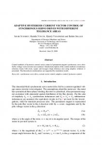
controller was developed for image-based dynamic control of a robot manipulator. One problem with methods based on the image-Jacobian is that the estimated image-Jacobian may contain singularities. The development in [49] exploits an additional potential force function to drive the estimated parameters away from the values that result in a singular Jacobian matrix. In [52], an adaptive homography-based controller was proposed to address problems of uncertainty in the intrinsic camera calibration parameters and lack of depth measurements. In Section VI-D, a combined high-gain control approach and an adaptive control strategy are proposed to regulate the robot end-effector to a desired pose asymptotically with considering this time-varying scaling factor. Robust control approaches based on static best-guess estimation of the calibration matrix have been developed to solve the uncalibrated visual servo regulation problem (cf. [18], [44], [50], [51]). Specifically, under a set of assumptions on the rotation and calibration matrix, a kinematic controller was developed in [44] that utilizes a constant, best-guess estimate of the calibration parameters to achieve local set-point regulation for the six degreeof-freedom visual servo control problem. Homography-based visual servoing methods using best-guess estimation are used in [18], [50], [51] to achieve asymptotic or exponential regulation with respect to both camera and hand-eye calibration errors for the six degree-of-freedom problem. This chapter is organized to provide the basic underlying principles of both historic and recent visual servo control methods with a progression to open research issues due to the loss of information through the image projection and the disturbances due to uncertainty in the camera calibration. Section IV provides an overview of the basic methodologies. This section includes topics such as: geometric relationships and Euclidean reconstruction using the homography in Section IV-A; and image-based visual servo control, position-based visual servo control, and hybrid visual servo control approaches in Sections IV-B-IV-D. In Section V, an adaptive technique that actively compensates for unknown depth parameters in visual servo control is presented. Specifically, this adaptive compensation approach has been combined with the homography-based visual servo control scheme and image-based visual servo control scheme to generate asymptotic results in Section V-A and V-B, respectively. In Section VI, several visual control approaches that do not require exact camera calibration knowledge are presented. For example, in Section VI-A, a visual servo controller that is based on a Jacobian matrix estimator is described. In Section VI-B, a robust controller based on static best-guess estimation of the calibration matrix is developed to solve the regulation problem. In Section VI-C, an adaptive controller for image-based dynamic regulation control of a robot manipulator is described based on a depth-independent interaction matrix. In Section VI-D, a combined high-gain control approach and an adaptive control strategy are used to regulate the robot end-effector to a desired pose based on the homography technique. IV. V ISUAL S ERVO C ONTROL M ETHODS The development in this chapter is focused on the development of visual servo controllers for robotic systems. To develop the controllers, the subsequent development is based on the assumption that images can be acquired, analyzed, and the resulting data can be provided to the controller without restricting the control rates. The sensor data from image-based feedback are feature points. Feature points are pixels in an image that can be identified and tracked between images so that the motion of the camera/robot can be discerned from the image. Image processing techniques can be used to select coplanar and non-collinear feature points within an image. For simplicity, the development in this chapter is based on the assumption that four stationary coplanar and non-collinear feature points [53] denoted by Oi ∀i = 1, 2, 3, 4 can be determined from a feature point tracking algorithm (e.g., KanadeLucas-Tomasi (KLT) algorithm discussed in [54] and [55]). The plane defined by the four feature points is denoted by π as depicted in Fig. 1. The assumption that feature points lie on a plane is not restrictive and does not reduce the generality of the results. For example, if four coplanar target points are not available then the subsequent development can also exploit methods such as the virtual parallax algorithm (e.g., see [16], [56]) to create virtual planes from non-planar feature points. A. Geometric Relationships The camera-in-hand configuration is depicted in Fig. 1. In Fig. 1, F denotes a coordinate frame that is considered to be affixed to the single current camera viewing the object, and a stationary coordinate frame F ∗ denotes a constant (a priori determined) desired camera position and orientation that is defined as a desired image. The Euclidean ¯ i (t) ∈ R3 and m ¯ ∗i ∈ R3 , coordinates of the feature points Oi expressed in the frames F and F ∗ are denoted by m respectively, as £ £ ¤T ¤T m ¯ i , xi (t) yi (t) zi (t) m ¯ ∗i , x∗i yi∗ zi∗ , (1)
6
Oi n* mi d*
π
m*i
F∗
xf, R
F Fig. 1.
Coordinate frame relationships between a camera viewing a planar patch at different spatiotemporal instances.
where xi (t), yi (t), zi (t) ∈ R denote the Euclidean coordinates of the ith feature point, and x∗i , yi∗ , zi∗ ∈ R denote the Euclidean coordinates of the corresponding feature points in the desired/reference image. From standard Euclidean geometry, relationships between m ¯ i (t) and m ¯ ∗i can be determined as m ¯ i = xf + Rm ¯ ∗i ,
(2)
where R (t) ∈ SO(3) denotes the orientation of F ∗ with respect to F , and xf (t) ∈ R3 denotes the translation vector from F to F ∗ expressed in the coordinate frame F . The normalized Euclidean coordinate vectors, denoted by mi (t) ∈ R3 and m∗i ∈ R3 , are defined as iT £ ¤T h xi yi 1 mxi myi 1 mi = , (3) zi zi ∙ ∗ ¸ T ¤T £ ∗ xi yi∗ 1 mxi m∗yi 1 m∗i = , . (4) zi∗ zi∗ Based on the Euclidean geometry in (2), the relationships between mi (t) and m∗i can be determined as [53] ´ xf zi∗ ³ R + ∗ n∗T m∗i mi = zi | d , {z } |{z} αi H
(5)
where αi (t) ∈ R is a scaling term, and H(t) ∈ R3×3 denotes the Euclidean homography. The Euclidean homography is composed of: a scaled translation vector which is equal to the translation vector xf (t) divided by the distance d∗ ∈ R from the origin of F ∗ to the plane π ; the rotation between F and F ∗ denoted by R (t); and n∗ ∈ R3 denoting a constant unit normal to the plane π . Each feature point Oi on π also has a pixel coordinate pi (t) ∈ R3 and p∗i ∈ R3 expressed in the image coordinate frame for the current image and the desired image denoted by £ £ ¤T ¤T pi , ui vi 1 p∗i , u∗i vi∗ 1 , (6) where ui (t), vi (t), u∗i , vi∗ ∈ R. The pixel coordinates pi (t) and p∗i are related to the normalized task-space coordinates mi (t) and m∗i by the following global invertible transformation (i.e., the pinhole camera model) pi = Ami
p∗i = Am∗i ,
(7)
7
where A ∈ R3×3 is a constant, upper triangular, and defined as [57] ⎡ α −α cot ϕ ⎢ β A,⎢ ⎣ 0 sin ϕ 0 0
invertible intrinsic camera calibration matrix that is explicitly ⎤ ⎡ ⎤ u0 a11 a12 a13 ⎥ ⎣ v0 ⎥ a22 a23 ⎦ , (8) ⎦= 0 0 0 1 1
where a11 , a12 , a13 , a22 , a23 ∈ R. In (8), u0 , v0 ∈ R denote the pixel coordinates of the principal point (i.e., the image center that is defined as the frame buffer coordinates of the intersection of the optical axis with the image plane), α, β ∈ R represent the product of the camera scaling factors and the focal length, and ϕ ∈ R is the skew angle between the camera axes. Based on the physical meaning, the diagonal calibration elements are positive (i.e., a11 , a22 > 0). Based on (7), the Euclidean relationship in (5) can be expressed in terms of the image coordinates as ¡ ¢ pi = αi AHA−1 p∗i | {z } , (9) G
where G(t) ∈ R3×3 denotes the projective homography. Based on the feature point pairs (p∗i , pi (t)) with i = 1, 2, 3, 4, the projective homography can be determined up G(t) where g33 (t) ∈ R denotes the bottom right element of G(t)) [19]. Various methods to a scalar multiple (i.e., g33 (t) can then be applied (e.g., see [58], [59]) to decompose the Euclidean homography to obtain the rotation matrix xf (t) R(t), scaled translation , normal vector n∗ , and the depth ratio αi (t). d∗ B. Image-based Visual Servo Control As described previously, image-based visual servo control uses pure image-space information (i.e., pixel coordinates) in the control development. The image error for the feature point Oi between the current and desired poses is defined as ∙ ¸ ui (t) − u∗i eii (t) = ∈ R2 . ∗ vi (t) − vvi
The derivative of eii (t) can be written as (e.g., see [3]–[5]) ∙ ¸ vc , e˙ ii = Lii ωc where Lii (mi , zi ) ∈ R2n×6 is defined as ⎡ ¸ −1 ∙ a11 a12 ⎢ zi Lii = ⎣ 0 a22 0
0 1 − zi
mxi zi myi zi
mxi myi 1 + m2yi
(10)
¢ ¡ − 1 + m2xi −mxi myi
myi −mxi
⎤
⎥ ⎦,
and vc (t), ω(t) ∈ R3 are linear and angular velocities of the camera, respectively, expressed in the camera coordinate frame F . If the image error is defined based on the normalized pixel coordinates as ¸ ∙ mxi (t) − m∗xi ∈ R2 eii (t) = myi (t) − m∗yi
then the derivative of eii (t) can be written as (e.g., see [13]) ⎡ ⎤ ¢ ¡ mxi 1 ¸ ∙ myi 0 mxi myi − 1 + m2xi − v ⎢ zi ⎥ c z i . e˙ ii = ⎣ (11) ⎦ 1 myi ωc 0 − 1 + m2yi −mxi myi −mxi zi zi £ ¤T The image error for n (n ≥ 3) feature points is defined as ei (t) = eTi1 (t) eTi2 (t) · · · eTin (t) ∈ R2n . Based on (10), the open-loop error system for ei (t) can be written as ∙ ¸ vc , e˙ i = Li (12) ωc
8
£ ¤T where the matrix Li (t) = LTi1 (t) LTi2 (t) · · · LTin (t) ∈ R2n×6 is called the image Jacobian, interaction matrix, feature sensitivity matrix, or feature Jacobian (cf. [2]–[5]). When the image Jacobian matrix is nonsingular at the desired point (i.e., ei (t) = 0), and the depth information zi (t) is available, a locally exponentially result (i.e., ei (t) → 0 exponentially) can be obtained by using the controller ∙ ¸ vc = −ki L+ (13) i ei , ωc
where ki ∈ R is a positive control gain, and L+ i (t) is the pseudoinverse of Li (t). See [13] for details regarding the stability analysis. In the controller (13), zi (t) is unknown. Direct approximation and estimation techniques (cf. [4], [5]) have been developed to estimate zi (t). For example, an approximate estimate of Li (t) using constant zi∗ at the desired pose has been used in [4]. Besides the direct approximation and estimation approaches, dynamic adaptive compensation approaches (cf. [19]–[22], [24]–[28]) have also been developed recently to compensate for this unknown depth information, which will be represented in Section V. C. Position-Based Visual Servo Control The feedback loop in position-based visual servo control (e.g., [1], [5], [9]–[11]) uses Euclidean pose information that is reconstructed from the image information. Various methods can be applied (cf. [5], [60], [61]) to compute the pose estimate based on the image information and a priori geometric knowledge of the environment. The resulting outcome of these methods are the translation vector xf (t) and rotation matrix R(t) between the current and desired poses of the robot end-effector. The rotation matrix can be further decomposed as a rotation axis u(t) ∈ R3 and a rotation angle θ(t) ∈ R. The pose error ep (t) ∈ R6 can be defined as ¸ ∙ xf , ep (t) = uθ where the corresponding open-loop error system can then be determined as ∙ ¸ vc , e˙ p = Lp ωc where Lp (t) ∈ R6×6 is defined as Lp =
In (15), Lω (u(t), θ(t)) ∈ R3×3 is defined as [15] Lω = I3 −
∙
R 0 0 Lω
⎛
⎜ θ [u]× + ⎜ ⎝1 − 2
¸
(14)
(15)
. ⎞
sinc (θ) ⎟ 2 µ ¶⎟ ⎠ [u]× . θ sinc 2 2
(16)
Based on the open-loop error system in (14), an example position-based visual servo controller can be designed as ∙ ¸ vc (17) = −kp L−1 p ep ωc
provided that Lp (t) is nonsingular, where kp ∈ R is a positive control gain. The controller in (17) yields an asymptotically stable result in the sense that ep (t) asymptotically converges to zero. See [13] for details regarding the stability analysis. A key issue with position-based visual servo control is the need to reconstruct the Euclidean information to find the pose estimate from the image. Given detailed geometric knowledge of the scene (such as a CAD model) approaches such as [5], [60], [61] can deliver pose estimates. When geometric knowledge is not available, homography-based Euclidean reconstruction is also a good option. Given a set of feature points as stated in Section IV-A and based on (5) and (7), the homography H(t) between the current pose and desired pose can be obtained if the camera calibration
9
matrix A is known. Various methods can then be applied (e.g., see [58], [59]) to decompose the homography to obtain xf (t) xf (t) the rotation matrices R(t) and the scaled translation vector . If is used in the control development, then ∗ d d∗ either d∗ should be estimated directly or adaptive control techniques would be required to compensate for/identify the unknown scalar. D. Homography-Based Visual Servo Control The 2.5D visual servo control approach developed in [15]–[18] decomposes the six-DOF motion into translation and rotation components and uses separate translation and rotation controllers to achieve the asymptotic regulation. This class of controllers is also called homography-based visual servo control in [19]–[22] because of the underlying reliance of the construction and decomposition of a homography. The translation error signal ev (t) ∈ R3 can be chosen as a combination of image information (or normalized Euclidean information) and reconstructed Euclidean information as µ ¶ ¸T ∙ zi ∗ ∗ ev = mxi − mxi myi − myi ln , (18) zi∗ where the current and desired Euclidean coordinates are related to the chosen feature point Oi . The rotation error signal eω (t) ∈ R3 is typically chosen in terms of the reconstructed rotation parameterization as eω = uθ.
The corresponding translation and rotation error system can be written as
where Lω (t) was defined in (16), ⎡ 1 αi ⎣ Lv = − ∗ 0 zi 0
e˙ v = Lv vc + Lvω ωc
(19)
e˙ ω = Lω ωc ,
(20)
and Lv (t), Lvω (t) ∈ R3×3 are defined as ⎤ ⎡ ⎤ mxi myi −1 − m2xi myi 0 −mxi 1 −myi ⎦ Lvω = ⎣ 1 + m2yi −mxi myi −mxi ⎦ . 0 1 −myi mxi 0
(21)
The rotation and translation controllers can be designed as
ω c = −kL−1 ω er = −keω vc =
−L−1 v (kev
(22)
− kLvω eω )
to yield an asymptotically stable result. There are some other control approaches that combine image-space and reconstructed Euclidean information in the error system such as [8], [23]. The partitioned visual servo control approach proposed in [8] decouples the z-axis motions (including both the translation and rotation components) from the other degrees of freedom and derives separate controllers for these z-axis motions. The switched visual servo control approach proposed in [23] partitions the control along the time axis, instead of the usual partitioning along spatial degrees of freedom. This system uses both position-based and image-based controllers, and a high-level decision maker invokes the appropriate controller based on the values of a set of Lyapunov functions. E. Simulation Comparisons The controllers given in (13), (17), and (22) are implemented based on the same initial conditions. The errors asymptotically converge for all three controllers. The different image-space and Euclidean trajectories in the simulation are shown in Fig. 2. Subplots (1)-(3) of Fig. 2 are two-dimensional image-space trajectories of the four feature points generated by the controllers (13), (17), and (22), respectively. The trajectories start from the initial positions and asymptotically converge to the desired positions. A comparison of the results indicate that the image-based visual servo control and homography-based visual servo control have better performance in the image-space (see subplots (1) and (3)).
500
500
450
450
450
400
400
400
350
350
350
300
300
300
250
v [pixle]
500
v [pixle]
v [pixle]
10
250 200
200
150
150
150
100
100
100
50
50
50
0
0
0
100
200 300 u [pixle]
400
500
0
100
200 300 u [pixle]
400
0
500
0
−2
−1.5
−1.5
−1.5
−1 −0.5
z [m]
−2
−1 −0.5
0 1
−1
−1
0 1
(4)
1 0
x [m]
500
−1
0 1 0
400
−0.5
1
y [m]
200 300 u [pixle]
(3)
−2
0
100
(2)
z [m]
z [m]
(1)
Fig. 2.
250
200
y [m]
0 −1
−1
x [m]
1 0 y [m]
0 −1
(5)
−1
x [m]
(6)
Simulation results for image-based, position-based, and combined visual servo cotnrol approaches.
Also, since the position-based visual servo controller does not use image-features in the feedback, the feature points may leave the camera’s field-of-view (see subplot (2)). Subplots (4)-(6) of Fig. 2 are the three-dimensional Euclidean trajectories of the camera generated by the controllers (13), (17), and (22), respectively. Since the position-based visual servo control uses the Euclidean information directly in the control loop, it has the best performance in the Euclidean trajectory (subplot (5)), followed by the homography-based controller (subplot (6)). The image-based visual servo controller in subplot (4) generates the longest Euclidean trajectory. Since image-based visual servo controller doesn’t guarantee the Euclidean performance, it may generate a physically unimplementable trajectory. V. C OMPENSATING FOR P ROJECTION N ORMALIZATION A key issue that impacts visual servo control is that the image-space is a two-dimensional projection of the threedimensional Euclidean-space. To compensate for the lack of depth information from the two-dimensional image data, some researchers have focused on the use of alternate sensors (e.g., laser and sound ranging technologies). Other researchers have explored the use of a camera-based vision system in conjunction with other sensors along with sensor fusion methods or the use of additional cameras in a stereo configuration that triangulate on corresponding images. However, the practical drawbacks of incorporating additional sensors include: increased cost, increased complexity, decreased reliability, and increased processing burden. Recently, some researchers have developed adaptive control methods that can actively adapt for the unknown depth parameter (cf. [19]–[22], [24]–[28]) along with methods based on direct estimation and approximation (cf. [4], [5]). A. Adaptive Depth Compensation in Homography-Based Visual Servo Control As in [19]–[22], [26]–[28], homography-based visual servo controllers have been developed to achieve asymptotic regulation or tracking control of a manipulator end-effector or a mobile robot, by developing an adaptive update law that actively compensates for an unknown depth parameter. The open-loop error system and control development are discussed in this section.
11
1) Open-Loop Error System: The translation error signal ev (t) is defined as in Section IV-D. However, the rotation ¤T £ ∈ R4 where q0 (t) ∈ R and qv (t) ∈ R3 (e.g., error signal is defined as a unit quaternion q(t) , q0 (t) qvT (t) see [22], [28]). The corresponding translation and rotation error systems are determined as ¯ v vc + zi∗ Lvω ω c zi∗ e˙ v = −αi L (23) and
∙
q˙0 q˙v
¸
1 = 2
∙
−qvT q0 I3 + qv×
¸
ωc,
(24)
¯ v (t) ∈ where the notation qv× (t) denotes the skew-symmetric form of the vector qv (t) (e.g., see [22], [28]), and L 3×3 is defined as R ⎤ ⎡ 1 0 −mxi ¯ v = ⎣ 0 1 −myi ⎦ . (25) L 0 0 1 ¯ v (t) is measurable and can be used in the controller development directly. The structure of (25) indicates that L 2) Controller and Adaptive Law Design: The rotation and translation controllers can be developed as (e.g., see [15], [19], [22], [28]) ω c = −Kω qv (26) 1 ¯ −1 vc = L (Kv ev + zˆi∗ Lvω ω c ) , (27) αi v where Kω , Kv ∈ R3×3 denote two diagonal matrices of positive constant control gains. In (27), the parameter estimate zˆi∗ (t) ∈ R is developed for the unknown constant zi∗ , and is defined as (e.g., see [19], [22], [28]) ·
zˆi∗ = γ i eTv Lvω ωc ,
(28)
where γ i ∈ R denotes a positive constant adaptation gain. Based on (23)-(28), the closed-loop error system is obtained as 1 T q Kω qv q˙0 = (29) 2 v ¢ 1¡ q˙v = − q0 I3 + qv× Kω qv (30) 2 zi∗ e˙ v = −Kv ev + z˜i Lvω ωc , (31) where z˜i (t) ∈ R denotes the following parameter estimation error: z˜i = zi∗ − zˆi∗ .
(32)
3) Closed-Loop Stability Analysis: The controller given in (26) and (27) along with the adaptive update law in (28) ensures asymptotic translation and rotation regulation in the sense that kqv (t)k → 0 and
kev (t)k → 0 as t → ∞.
To prove the stability result, a Lyapunov function candidate V (t) ∈ R can be defined as z∗ 1 2 V = i eTv ev + qvT qv + (1 − q0 )2 + z˜ . 2 2γ i i The time-derivative of V (t) can be determined as ¡ ¢ V˙ = eTv (−Kv ev + z˜i Lvω ωc ) − qvT q0 I3 + qv× Kω qv − (1 − q0 )qvT Kω qv − z˜i eTv Lvω ω c ,
(33)
(34)
(35)
where (29)-(32) were utilized. The following negative semi-definite expression is obtained after simplifying (35): (36) V˙ = −eTv Kv ev − qvT Kω qv .
Barbalat’s Lemma [62] can then be used to prove the result given in (33). Based on the controller in (26) and (27) and the adaptive law in (28), the resulting asymptotic translation and rotation errors are plotted in Fig. 3 and Fig. 4, respectively. The image-space trajectory is shown in Fig. 5, and also in Fig. 6 in a three-dimensional format, where the vertical axis is time. The parameter estimate for zi∗ is shown in Fig. 7.
12
ev1
0 −0.02 −0.04 −0.06
0
2
4
6
8
10
0
2
4
6
8
10
0
2
4
6
8
10
ev2
0 −0.05 −0.1
ev3
0 −0.2 −0.4
Time [sec]
Fig. 3.
Unitless translation error ev (t).
q0
1 0.8 0.6 0
2
4
6
8
10
0
2
4
6
8
10
0
2
4
6
8
10
0
2
4
6
8
10
qv1
0.5 0 −0.5
qv2
0.5 0 −0.5
qv3
0 −0.5 −1
Time [sec]
Fig. 4.
Quaternion rotation error q(t).
B. Adaptive Depth Compensation in Image-Based Visual Servo Control This section provides an example of how an image-based visual servo controller can be developed that adaptively compensates for the uncertain depth. In this section, only three feature points are required to be tracked in the image to develop the error system (i.e., to obtain an image-Jacobian with at least equal rows than columns), but at least four feature points are required to solve for the unknown depth ratio αi (t). 1) Open-Loop Error System: The image error ei (t) defined in Section IV-B can be rewritten as ⎡ ⎤ ⎡ ⎤ mx1 (t) − m∗x1 ex1 ⎢ my1 (t) − m∗y1 ⎥ ⎢ ey1 ⎥ ⎢ ⎥ ⎢ ⎥ ⎢ mx2 (t) − m∗x2 ⎥ ⎢ ex2 ⎥ ⎢ ⎢ ⎥ ⎥, ei (t) = ⎢ (37) ∗ ⎥,⎢ ⎥ m (t) − m e y2 y2 y2 ⎢ ⎥ ⎢ ⎥ ⎣ mx3 (t) − m∗ ⎦ ⎣ ex3 ⎦ x3 ey3 my3 (t) − m∗y3
13
138 136 134
vi [pixel]
132 130 128 p2(0) p1(0)
126 p3(0)
p4(0)
124 122 120
122
124
126
128 u [pixel]
130
132
134
136
i
Fig. 5. Image-space error in pixles between p(t) and p∗ . In the figure, “O” denotes the initial positions of the 4 feature points in the image, and “*” denotes the corresponding final positions of the feature points.
10
Time [sec]
8 6 4 2 0 140 135
140
p1(0) p2(0)
130
p4(0) 125
v [pixel] i
p3(0) 120
120
135 130
125 ui [pixel]
Fig. 6. Image-space error in pixles between p(t) and p∗ shown in a 3D graph. In the figure, “O” denotes the initial positions of the 4 feature points in the image, and “*” denotes the corresponding final positions of the feature points.
when three feature points are used for notation simplicity. The definition of image error ei (t) is expandable to more than three feature points. The time derivative of ei (t) is given by ∙ ¸ vc e˙ i (t) = Li (38) , ωc
14
0.6004 0.6002 0.6 0.5998
[m]
0.5996 0.5994 0.5992 0.599 0.5988 0.5986
0
2
4
6
8
10
Time [sec]
Fig. 7.
Adaptive on-line estimate of zi∗ .
where the image Jacobian Li (t) is given by ⎡ α 1 0 z∗ ⎢ 01 α1 ∗ ⎢ ⎢ α2 z1 ⎢ z∗ 0 2 Li = ⎢ ⎢ 0 α∗2 ⎢ z ⎢ α3 02 ⎣ z3∗ 0 αz∗3
α1 mx1 z1∗ α1 m y1 z1∗ α2 mx2 z2∗ α2 m y2 z2∗ α3 mx3 z3∗ α3 m y3 z3∗
1 + m2x1 mx1 my1 1 + m2x2 mx2 my2 1 + m2x3 mx3 my3 3 £ where the depth ratio αi (t), i = 1, 2, 3 is defined in (5). Let φ = φ1 constant parameter vector as h i φ=
−mx1 my1 −1 − m2y1 −mx2 my2 −1 − m2y2 −mx3 my3 −1 − m2y3
1 z1∗
1 z2∗
1 z3∗
T
.
−my1 mx1 −my2 mx2 −my3 mx3 φ2 φ3
⎤
⎥ ⎥ ⎥ ⎥ ⎥, ⎥ ⎥ ⎥ ⎦
¤T
(39)
∈ R3 denote the unknown
(40)
Even though the error system (38) is not linearly parameterizable in φ, an adaptive law can still be developed based on the following property in Section V-B.2. 2) Controller and Adaptive Law Design : Based on an open-loop error system as in (38), the controller is developed as ∙ ¸ vc ˆ Ti ei , = −ki L (41) ωc £ ¤ ˆ (t) = φ ˆ (t) φ ˆ (t) φ ˆ (t) T ∈ R3 is the adaptive estimation of the where ki ∈ R is the control gain, φ 1 2 3 ˆ i (t) ∈ R6×6 is an estimation of the image Jacobian unknown constant parameter vector defined in (40), and L matrix as ⎡ ⎤ ˆ ˆ −mx1 my1 1 + m2 −my1 α1 φ 0 α1 mx1 φ 1 1 x1 ⎢ 0 ˆ ˆ −1 − m2 mx1 my1 mx1 ⎥ φ α1 my1 φ 1 1 ⎢ ⎥ y1 ⎢ ⎥ 2 ˆ ˆ α 0 α m −m m 1 + m −m φ φ ⎢ 2 x2 2 x2 y2 y2 ⎥ x2 ˆi = ⎢ 2 2 . (42) L ˆ −1 − m2 mx2 my2 mx2 ⎥ ˆ ⎢ 0 ⎥ φ α2 my2 φ 2 2 y2 ⎢ ⎥ ˆ3 ˆ 3 −mx3 my3 1 + m2 −my3 ⎦ ⎣ α3 φ 0 α3 mx3 φ x3 ˆ ˆ 0 α3 φ3 α3 my3 φ3 −1 − m2y3 mx3 my3 mx3 ˆ The adaptive law for φ(t) in (42) is designed as ·
ˆ = −ΓeM L ˆ iM L ˆ Ti ei , φ
(43)
15
ˆ iM (t) ∈ R6×6 are defined as where Γ ∈ R3×3 is a positive diagonal matrix, eM (t) ∈ R3×6 and L ⎡ α1 0 mx1 α1 0 0 0 ⎢ 0 α1 my1 α1 0 0 0 ⎡ ⎤ ⎢ ex1 ey1 0 0 0 0 ⎢ ˆ iM = ⎢ α2 0 mx2 α2 0 0 0 0 ex2 ey2 0 0 ⎦ eM = ⎣ 0 L ⎢ 0 α2 my2 α2 0 0 0 ⎢ 0 0 0 0 ex3 ey3 ⎣ α3 0 mx3 α3 0 0 0 0 α3 my3 α3 0 0 0
The adaptive law is motivated by the following two properties:
⎤
⎥ ⎥ ⎥ ⎥. ⎥ ⎥ ⎦
ˆi = L ˜ i = ΦM L ˆ iM Li − L T ˜ eM L ˆ iM = φ ˆ iM . eTi ΦM L
(44) (45)
˜ ∈ R3 and ΦM (t) ∈ R6×6 are defined as In (44) and (45), the adaptive estimation error φ(t) £ £ ¤ ¤ ˜ = ˜ φ ˜ T = φ −φ ˜ φ ˆ φ −φ ˆ φ −φ ˆ T φ φ 1 2 3 1 1 2 2 3 3 o n ˜1, φ ˜1, φ ˜2, φ ˜2, φ ˜3, φ ˜3 . ΦM = diag φ
Under the controller (41) and the adaptive law (43), the closed-loop error system can be written as · ˆ Ti ei = −ki L ˆiL ˆ Ti ei − ki L ˜iL ˆ Ti ei = −ki L ˆ iL ˆ Ti ei − ki ΦM L ˆ iM L ˆ Ti ei . ei = −ki Li L
(46)
3) Closed-Loop Stability Analysis: The controller given in (41) and the adaptive update law in (43) ensures asymptotic regulation in the sense that kei (t)k → 0 as t → ∞. (47) To prove the stability result, a Lyapunov function candidate V (t) ∈ R can be defined as
1 1 ˜ −1 ˜ V = eTi ei + ki φΓ φ. 2 2 The time-derivative of V (t) can be determined as V˙
·
· ˜ −1 φ ˆ = eTi ei − ki φΓ ³ ´ ³ ´ ˜ −1 ΓeM L ˆ iL ˆ Ti ei − ki ΦM L ˆ iM L ˆ Ti ei − ki φΓ ˆ iM ei = eTi −ki L
˜ ML ˆ iL ˆ Ti ei − ki eTi ΦM L ˆ iM L ˆ Ti ei + ki φe ˆ iM L ˆ Ti ei . = −ki eTi L
Based on (44) and (45)
˜ T eM L ˆ iM L ˆ Ti = φ ˆ iM L ˆ Ti , eTi ΦM L
and V˙ (t) can be further simplified as ˜ ML ˜ ML ˆ iL ˆ Ti ei − ki φe ˆ iM L ˆ Ti ei + ki φe ˆ iM L ˆ Ti ei = −ki eTi L ˆ iL ˆ Ti ei . V˙ = −ki eTi L
Barbalat’s Lemma [62] can then be used to conclude the result given in (47). VI. V ISUAL S ERVO C ONTROL VIA AN U NCALIBRATED C AMERA Motivated by the desire to incorporate robustness to camera calibration, different control approaches (e.g., Jacobian estimation-based least-square optimization, robust control, and adaptive control) that do not depend on exact camera calibration have been proposed (cf. [18], [36]–[51], [63]).
16
A. Jacobian Estimation Approach The uncalibrated visual servo controllers that are based on a Jacobian matrix estimator have been developed in [36]–[40]. The camera calibration matrix and kinematic model is not required with the Jacobian matrix estimation. This type of visual servo control scheme is composed of a recursive Jacobian estimation law and a control law. Specifically, in [36], a weighted recursive least-square update law is used for Jacobian estimation, and a visual servo controller is developed via the Lyapunov approach. In [37], a Broyden Jacobian estimator is applied for Jacobian estimation and a nonlinear least-square optimization method is used for the visual servo controller development. In [39] and [40] a recursive least-squares algorithm is implemented for Jacobian estimation, and a dynamic GaussNewton method is used to minimize the squared error in the image plane to get the controller. Let the robot end-effector features y(θ) ∈ Rm be a function of the robot joint angle vector θ (t) ∈ Rn , and let the target features y∗ (t) ∈ Rm be a function of time. The tracking error in the image-plane can then be defined as f (θ, t) = y (θ) − y ∗ (t) ∈ Rm .
The trajectory θ (t) that causes the end-effector to follow the target is established by minimizing the squared image error 1 F (θ, t) = f T (θ, t) f (θ, t) . 2 By using the dynamic Gauss-Newton method, the joint angle vector update law (controller) can be designed as [40] µ ¶ ³ ´−1 ∂fk ht θk+1 = θk − JˆkT Jˆk (48) JˆkT fk + ∂t
ˆ , can be determined by multiple recursive where ht is the increment of t. In (48), the estimated Jacobian J(t) least-square Jacobian estimation algorithms (e.g., Broyden method [37], dynamic Broyden method [40], or an exponentially weighted recursive least-square algorithm [40]).
B. Robust Control Approach Robust control approaches based on static best-guess estimation of the calibration matrix have been developed to solve the uncalibrated visual servo regulation problem (cf. [18], [44], [50], [51]). Specifically, a kinematic controller was developed in [44] that utilizes a constant, best-guess estimate of the calibration parameters to achieve local set-point regulation for the six-DOF problem; although, several conditions on the rotation and calibration matrix are required. Model-free homography-based visual servoing methods using best-guess estimation are used in [18] and [50] to achieve exponential or asymptotic regulation with respect to both camera and hand-eye calibration errors for the six-DOF problem. A quaternion-based robust controller is developed in [51] that achieved a regulation control objective. 1) State Estimation: Let Aˆ ∈ R3×3 be a constant best-guess estimate of the camera calibration matrix A. The normalized coordinate estimates, denoted by m ˆ i (t) , m ˆ ∗i ∈ R3 , can be expressed as ˜ i m ˆ i = Aˆ−1 pi = Am
(49)
˜ ∗i m ˆ ∗i = Aˆ−1 p∗i = Am
(50)
where the upper triangular calibration error matrix A˜ ∈ R3×3 is defined as A˜ = Aˆ−1 A.
(51)
Since mi (t) and m∗i can not be exactly determined, the estimates in (49) and (50) can be substituted into (5) to obtain the following relationship: ˆm m ˆ i = αi H (52) ˆ ∗i , ˆ (t) ∈ R3×3 denotes the estimated Euclidean homography [18] defined as where H ˆ = AH ˜ A˜−1 . H
(53)
Since m ˆ i (t) and m ˆ ∗i can be determined from (49) and (50), a set of twelve linear equations can be developed from ˆ (t). If additional information (e.g., at least four the four image point pairs, and (52) can be used to solve for H
17
vanishing points) is provided (see [64] for a description of how to determine vanishing points in an image), various ˆ techniques (e.g., see [58], [59]) can be used to decompose H(t) to obtain the estimated rotation and translation components as ˜ h n∗T A˜−1 = R ˆ+x ˆ = AR ˜ A˜−1 + Ax ˆh n ˆ ∗T , (54) H ˆ (t) ∈ R3×3 and x ˆh (t) , n ˆ ∗ ∈ R3 denote the estimate of R(t), xh (t) and n∗ , respectively, as [18] where R
where σ ∈ R denotes the positive constant
ˆ = AR ˜ A˜−1 , R
(55)
˜ h, x ˆh = σ Ax 1 n ˆ ∗ = A˜−T n∗ , σ
(56)
° ° ° ˜−T ∗ ° σ = °A n ° .
(57) (58)
ˆ (t) is similar to R (t). By exploiting the properties of similar Based on (55), the rotation matrix estimate R matrices (i.e., similar matrices have the same trace and eigenvalues), the following estimates can be determined as [18] ˆ ˜ θ=θ u ˆ = μAu,
where ˆθ (t) ∈ R and u ˆ (t) ∈ R3 denote the estimates of θ(t) and u (t), respectively, and μ ∈ R is defined as 1 ° μ= ° ° ˜ °. °Au°
Alternatively, if the rotation matrix is decomposed as a unit quaternion. The quaternion estimate ¤T £ qˆ(t) , qˆ0 (t) qˆvT (t) ∈ R4 can be related to the actual quaternion q (t) as [51]
qˆ0 = q0
where
˜ v, qˆv = ±μAq
kqv k ° μ= ° ° ˜ °. °Aqv °
(59) (60)
Since the sign ambiguity in (59) does not affect the control development and stability analysis [51], only the positive sign in (59) needs to be considered in the following control development and stability analysis. 2) Control Development and Stability Analysis: The rotation open-loop error system can be developed by taking the time derivative of q(t) as ∙ ∙ ¸ ¸ 1 q˙0 −qvT = ωc. (61) q˙v 2 q0 I3 + qv× Based on the open-loop error system in (61) and the subsequent stability analysis, the angular velocity controller is designed as ω c = −kω qˆv , (62)
where kω ∈ R denotes a positive control gain. Substituting (62) into (61), the rotation closed-loop error system can be developed as 1 kω qvT qˆv q˙0 = (63) 2 ¢ 1 ¡ q˙v = − kω q0 I3 + qv× qˆv . (64) 2 The open-loop translation error system can be determined as [50] 1 ∗ × e˙ = − ∗ vc − ω× (65) c e + [mi ] ω c , zi
18
where the translation error e (t) ∈ R3 is defined as e=
zi mi − m∗i . zi∗
The translation controller is designed as (see also [18], [50]) (66)
vc = kv eˆ,
where kv ∈ R denotes a positive control gain, and eˆ (t) ∈ R3 is defined as zi eˆ = ∗ m ˆi −m ˆ ∗i . zi ˆ i (t) and m ˆ ∗i can be computed from (49) and (50), respectively, and the ratio In (67), m
(67) zi (t) can be computed from zi∗
the decomposition of the estimated Euclidean homography in (52). After substituting (62) and (66) into (65), the resulting closed-loop translation error system can be determined as µ ¶ 1 ˜ × e˙ = −kv ∗ A + [kω qˆv ] (68) e − kω [m∗i ]× qˆv . zi
The controller given in (62) and (66) ensures asymptotic regulation in the sense that kqv (t)k → 0,
ke(t)k → 0
as t → ∞
(69)
provided kv is selected sufficiently large, and the following inequalities are satisfied (cf. [18], [50], [51]) ¾ ¾ ½ ³ ½ ³ 1 ˜ ˜T ´ 1 ˜ ˜T ´ ≥ λ0 ≤ λ1 , λmin λmax A+A A+A 2 2
where³ λ0 , λ1 ∈´R are positive constants, and λmin {·} and λmax {·} denote the minimal and maximal eigenvalues 1 ˜ ˜T of A + A , respectively. 2 To prove the stability result, a Lyapunov function candidate V (t) ∈ R can be defined as V = qvT qv + (1 − q0 )2 + eT e.
(70)
The time derivative of (70) can be proven to be negative semi-definite as [51] λ0 kω λ0 μ kqv k2 − ∗ kek2 , V˙ ≤ − Kv1 zi
(71)
where Kv1 is a positive large enough number. Using the signal chasing argument in [51], Barbalat’s Lemma [62] can then be used to prove the result given in (69). Based on the controller in (62) and (66), the resulting asymptotic translation and rotation errors are plotted in Fig. 8 and Fig. 9, respectively. C. Adaptive Image-Based Visual Servo Control Approach In [49], an adaptive controller for image-based dynamic regulation control of a robot manipulator is proposed using a fixed camera whose intrinsic and extrinsic parameters are not known. A novel depth-independent interaction matrix (cf. [49], [65], [66]) is proposed therein to map the visual signals onto the joints of the robot manipulator. Due to the depth-independent interaction matrix, the closed-loop dynamics can be linearly parameterized in the constant unknown camera parameters. An adaptive law can then be developed to estimate these parameters online.
19
e1
0 −0.1 −0.2
0
2
4
6
8
10
0
2
4
6
8
10
0
2
4
6
8
10
e2
0 −0.1 −0.2
e3
0.5 0 −0.5
Time [sec]
Fig. 8.
Unitless translation error between m1 (t) and m∗1 .
q0
1 0.8 0.6 0
2
4
6
8
10
0
2
4
6
8
10
0
2
4
6
8
10
0
2
4
6
8
10
qv1
0.2 0 −0.2
qv2
0 −0.1 −0.2
qv3
0 −0.5 −1
Time [sec]
Fig. 9.
Quaternion rotation error q(t).
1) Open-Loop Error System: Denote the homogeneous coordinate of the feature point expressed in the robot base frame as £ ¤T x ¯ (t) = x (t) y (t) z (t) 1 ∈ R4 , and denote its coordinate in the camera frame as £ c x ¯ (t) = c x (t)
c y (t)
c z (t)
¤T
∈ R3 .
The current and desired positions of the feature point on the image plane are respectively defined as £ ¤T £ ¤T p (t) = u (t) v (t) 1 ∈ R3 and pd = ud vd 1 ∈ R3 .
The image error between the current and desired positions of the feature point on the image plane, denoted as ei (t) ∈ R3 , is defined as £ ¤T £ ¤T ei = p − pd = u v 1 − ud vd 1 . (72)
20
Under the camera perspective projection model, p(t) can be related to x ¯ (t) as p=
1 cz
Mx ¯ (t) ,
(73)
where M ∈ R3×4 is a constant perspective projection matrix that depends only on the intrinsic and extrinsic calibration parameters. Based on (73), the depth of the feature point in the camera frame is given by c
z (t) = mT3 x ¯ (t) ,
(74) ·
¯ (t) where m3 ∈ R1×4 is the third row of M . Based on (72)-(74), the derivative of image error e˙ i (t) is related to x as ¢· 1 ¡ e˙ i = p˙ = c M − pmT3 x ¯. (75) z The robot kinematics are given by · x ¯ = J(q)q, ˙ (76)
where q(t) ∈ Rn denotes the joint angle of the manipulator, and J(q) ∈ R4×n denotes the manipulator Jacobian. Based on (75) and (76), ¢ 1 ¡ e˙ i = c M − pmT3 J(q)q. (77) ˙ z The robot dynamics are given by µ ¶ 1 ˙ H (q) q¨ + (78) H (q) + C (q, q) ˙ q˙ + g(q) = τ . 2
In (78), H (q) ∈ Rn×n is the positive-definite and symmetric inertia matrix, C (q, q) ˙ ∈ Rn×n is a skew-symmetric matrix, g(q) ∈ Rn denotes the gravitational force, and τ (t) ∈ Rn is the joint input of the robot manipulator. 2) Controller and Adaptive Law Design: As stated in Property 2 of [49], the perspective projection matrix M can only be determined up to a scale, so it is reasonable to fix one component of M and treat the others as unknown constant parameters. Without loss of generality, let m34 be fixed, and define the unknown parameter vector as £ ¤T φ = m11 m12 m13 m14 m21 m22 m23 m24 m31 m32 m33 ∈ R11 . To design the adaptive law, the estimated projection error of the feature point is defined as ˜ ˆ (t)¯ e(tj , t) = p(tj )m ˆ T3 (t)¯ x(tj ) − M x(tj ) = W (¯ x(tj ), p(tj )) φ
(79)
at time instant tj . In (79), W (¯ x(tj ), p(tj )) ∈ R3×11 is a constant regression matrix and the estimation error ˜ ∈ R11 is defined as φ(t) ˜ = φ−φ ˆ (t) with φ ˆ (t) ∈ R11 equal to the estimation of φ. The controller can then φ(t) be designed as [49] µ ¶ 1 T T T ˆ τ = g(q) − K1 q˙ − J (q) M − m ˆ 3p + m (80) ˆ 3 ei Bei 2 where K1 ∈ Rn×n and B ∈ R3×3 are positive-definite gain matrices. The adaptive law is designed as · ¢ ¡ ˆ = −Γ−1 Y T (q, p) q˙ + Σm W T (¯ φ x(tj ), p(tj )) K3 e(tj , t j=1
(81)
where Γ ∈ R11×11 and K3 ∈ R3×3 are positive-definite gain matrices, and the regression matrix Y (q, p) is determined as ¸ ∙³ ´ 1 T T T T T T ˜ ˆ ˆ 3 − m3 ) ei Bei = Y (q, p) φ. −J (q) M − m ˆ 3 p − M + m3 p + (m 2
As stated in [49], if the five positions (corresponding to five time instant tj , j = 1, 2, ..., 5) of the feature point for the parameter adaptation are so selected that it is impossible to find three collinear projections on the image plane, under the control of the proposed controller (80) and the adaptive algorithm (81) for parameter estimation, then the image error of the feature point is convergent to zero, i.e., kei (t)k → 0 as t → ∞ (see [49] for the closed-loop stability analysis).
21
D. Adaptive Homography-Based Visual Servo Control Approach 1) Problem Statement and Assumptions: In this section, a combined high-gain control approach and an adaptive control strategy are used to regulate the robot end-effector to a desired pose asymptotically. A homography-based visual servo control approach is used to address the six-DOF regulation problem. A high-gain controller is developed to asymptotically stabilize the rotation error system by exploiting the upper triangular form of the rotation error system and the fact that the diagonal elements of the camera calibration matrix are positive. The translation error system can be linearly parameterized in terms of some unknown constant parameters which are determined by the unknown depth information and the camera calibration parameters. An adaptive controller is developed to stabilize the translation error by compensating for the unknown depth information and intrinsic camera calibration parameters. A Lyapunov-based analysis is used to examine the stability of the developed controller. The following development is based on two mild assumptions. Assumption 1: The bounds of a11 and a22 (defined in Section IV-A) are assumed to be known as ζ a < a11 < ζ a11 11
ζ a < a22 < ζ a22 . 22
(82)
The absolute values of a12 , a13 , and a23 are upper bounded as |a12 | < ζ a12
|a13 | < ζ a13
|a23 | < ζ a23 .
(83)
In (82) and (83), ζ a , ζ a11 , ζ a , ζ a22 , ζ a12 , ζ a13 and ζ a23 are positive constants. 11 22 Assumption 2: The reference plane is within the camera field-of-view and not at infinity. That is, there exist positive constants ζ z and ζ zi such that i ζ z < zi (t) < ζ zi . (84) i
2) Euclidean Reconstruction Using Vanishing Points: Based on (5)-(7), the homography relationship based on measurable pixel coordinates is pi = αi AHA−1 p∗i . (85) Since A is unknown, standard homography computation and decomposition algorithms can’t be applied to extract the rotation and translation from the homography. If some additional information can be applied (e.g., four vanishing points), the rotation matrix can be obtained. For the vanishing points, d∗ = ∞, so that xf H = R + ∗ n∗T = R. (86) d Based on (86), the relationship in (85) can be expressed as ¯ ∗i , pi = αi Rp (87) ¯ (t) ∈ R3×3 is defined as where R
¯ = ARA−1 . R
(88)
¯ by For the four vanishing points, twelve linear equations can be obtained based on (87). After normalizing R(t) ¯ ¯ one nonzero element (e.g., R33 (t) ∈ R which is assumed to be the third row third column element of R(t) without loss of generality) twelve equations can be used to solve for twelve unknowns. The twelve unknowns are given by ¯ , denoted by R ¯ n (t) ∈ R3×3 defined as the eight unknown elements of the normalized R(t) ¯ ¯n , R , (89) R ¯ 33 R ¯ 33 (t)αi (t). From the definition of R ¯ n (t) in (89), the fact that and the four unknowns are given by R ¡ ¢ ¯ = det(A) det(R) det(A−1 ) = 1 det R (90)
can be used to conclude that and hence,
¡ ¢ 3 ¯ n = 1, ¯ 33 det R R ¯ ¯ = p Rn . R 3 ¯n) det(R
(91) (92)
¯ (t) is obtained, the original four feature points on the reference plane can be used to determine the depth After R ratio αi (t).
22
3) Open-Loop Error System: a) Rotation Error System: If the rotation matrix R (t) introduced in (5) were known, then the corresponding ¤T £ can be calculated using the numerically robust method presented in [28] unit quaternion q (t) , q0 (t) qvT (t) and [67] based on the corresponding relationships ¡ ¢ R (q) = q02 − qvT qv I3 + 2qv qvT − 2q0 qv× , (93)
where I3 is the 3 × 3 identity matrix, and the notation qv× (t) denotes the skew-symmetric form of the vector qv (t). Given R(t), the quaternion q(t) can also be written as 1p 1 p q0 = 1 + tr(R) qv = u 3 − tr(R), (94) 2 2 where u(t) ∈ R3 is a unit eigenvector of R(t) with respect to the eigenvalue 1. The open-loop rotation error system for q(t) can be obtained as [68] ∙ ∙ ¸ ¸ 1 q˙0 −qvT = ωc, (95) q˙v 2 q0 I3 + qv×
where ω c (t) ∈ R3 defines the angular velocity of the camera expressed in F . ¯ The quaternion q (t) given in (93)-(95) is not measurable since R(t) is unknown. However, since R(t) can be determined as described in (92), the same algorithm as shown in equation (94) can be used to determine a ¢T ¡ T corresponding measurable quaternion q¯0 (t), q¯v (t) as q q 1 1 ¯ ¯ ¯ 3 − tr(R), q¯0 = 1 + tr(R) q¯v = u (96) 2 2 ¡ ¢ ¯ = ¯ where ¯(t) ¢ ∈ R3 is a unit eigenvector of R(t) with respect to the eigenvalue 1. Based on (88), tr R ¡ u −1 ¯ = tr(R), where tr (·) denotes the trace of a matrix. Since R(t) and R(t) are similar matrices, tr ARA ¢T ¢T ¡ ¡ the relationship between q0 (t), qvT (t) and q¯0 (t), q¯vT (t) can be determined as q¯0 = q0
q¯v =
kqv k Aqv , γAqv , kAqv k
where γ(t) ∈ R is a positive, unknown, time-varying scalar. The square of γ(t) is qvT qv qvT qv γ2 = = . qvT AT Aqv (Aqv )T Aqv
(97)
(98)
Since A is of full rank, the symmetric matrix AT A is positive definite. Hence, the Rayleigh-Ritz theorem can be used to conclude that λmin (AT A)qvT qv ≤ qvT AT Aqv ≤ λmax (AT A)qvT qv . (99) From (98) and (99), it can be concluded that
1 qvT qv 1 2 ≤ γ . = ≤ T T λmax (A A) λmin (AT A) (Aqv ) Aqv s s 1 1 ≤γ≤ . T λmax (A A) λmin (AT A)
(100)
Based on (100), there exist positive bounding constants ζ γ , ζ γ ∈ R that satisfy the following inequalities: ζ γ < γ(t) < ζ γ .
The inverse of the relationship between q¯v (t) and qv (t) in (97) can also be developed as ¶ µ ⎡ ⎤ 1 a12 a13 a12 a23 q¯v3 q¯v1 − q¯v2 − − ⎥ a11 a22 a11 a11 a22 1 1⎢ ⎢ a11 ⎥ 1 a23 qv = A−1 q¯v = ⎢ ⎥. q¯v2 − q¯v3 γ γ⎣ ⎦ a22 a22 q¯v3
(101)
(102)
23
b) Translation Error System: The translation error, denoted by e(t) ∈ R3 , is defined as e(t) = pe (t) − p∗e ,
where pe (t), p∗e ∈ R3 are defined as £ ¤T pe = ui vi − ln (αi )
p∗e =
(103) £
u∗i vi∗ 0
¤T
(104)
,
where i ∈ {1, · · · , 4}. The translation error e(t) is measurable since the first two elements are image coordinates, and αi (t) is obtained from the homography decomposition. The open-loop translation error system can be obtained by taking the time derivative of e(t) and multiplying the resulting expression by zi∗ as ¡ ¢× zi∗ e˙ = −αi Ae vc + zi∗ Ae A−1 pi ωc , (105) where vc (t) ∈ R3 defines the linear velocity of the camera ⎡ a11 a12 ⎣ a22 Ae = 0 0 0
expressed in F , and Ae (t) ∈ R3×3 is defined as ⎤ a13 − ui a23 − vi ⎦ . 1
4) Rotation Controller Development and Stability Analysis : Based on the relationship in (97), the open-loop error system in (95), and the subsequent stability analysis, the rotation controller is designed as (106)
ωc1 = −kω1 q¯v1 = − (kω11 + 2) q¯v1
ωc2 = −kω2 q¯v2 = − (kω21 + kω22 + 1) q¯v2
ωc3 = −kω3 q¯v3 = − (kω31 + kω32 + kω33 ) q¯v3 ,
where kωi ∈ R, i = 1, 2, 3 and kωij ∈ R, i, j = 1, 2, 3, j < i, are positive constants. The expressed form of the controller in (106) is motivated by the use of completing the squares in the subsequent stability analysis. In (106), the damping control gains kω21 , kω31 , kω32 are selected according to the following sufficient conditions to facilitate the subsequent stability analysis à !2 2 2 ζ a12 ζ a23 1 2 ζ a12 1 2 1 1 2 ζ a23 kω21 > kω1 kω31 > kω1 + ζ a13 kω32 > kω2 , (107) 4 ζa ζa 4 ζa ζa 4 ζa 11
22
11
22
22
where ζ a , ζ a11 , ζ a , ζ a22 , ζ a12 , ζ a13 and ζ a23 are defined in (82) and (83), and kω11 , kω22 , kω33 are feedback 11 22 gains that can be selected to adjust the performance of the rotation control system. Provided the sufficient gain conditions given in (107) are satisfied, the controller in (106) ensures asymptotic regulation of the rotation error in the sense that kqv (t)k → 0,
as t → ∞.
(108)
To prove the stability result, a Lyapunov function candidate V1 (t) ∈ R can be defined as V1 , qvT qv + (1 − q0 )2 .
(109)
Based on the open-loop error system in (95), the time-derivative of V1 (t) can be determined as V˙ 1 = 2qvT q˙v − 2(1 − q0 )q˙0 = qvT ω c = qv1 ω c1 + qv2 ω c2 + qv3 ω c3 .
(110)
After substituting (102) for qv (t), substituting (106) for ω c (t), and completing the squares, the expression in (110) can be written as µ ¶ 1 2 1 2 1 2 ˙ q¯ + kω22 q¯ + kω33 q¯v3 . (111) V1 < − kω11 a11 v1 a22 v2 ζγ Barbalat’s lemma [62] can now be used to conclude that kqv (t)k → 0 as t → ∞.
24
5) Translation Control Development and Stability Analysis : After some algebraic manipulation, the translation error system in (105) can be rewritten as zi∗ e˙ 1 = −αi vc1 + Y1 (αi , ui , vi , ω c , vc2 , vc3 ) φ1 a11 zi∗ e˙ 2 = −αi vc2 + Y2 (αi , ui , vi , ω c , vc3 ) φ2 a22 zi∗ e˙ 3 = −αi vc3 + Y3 (αi , ui , vi , ω c ) φ3 ,
(112)
where φ1 ∈ Rn1 , φ2 ∈ Rn2 , and φ3 ∈ Rn3 are vectors of constant unknown parameters, and Y1 (·) ∈ R1×n1 , Y2 (·) ∈ R1×n2 , and Y3 (·) ∈ R1×n3 are known regressor vectors. The control strategy used in [52] is to design vc3 (t) to stabilize e3 (t), and then design vc2 (t) to stabilize e2 (t) given vc3 (t), and then design vc1 (t) to stabilize e1 (t) given vc3 (t) and vc2 (t). Following this design strategy, the translation controller vc (t) is designed as [52] ´ 1 ³ ˆ kv3 e3 + Y3 (αi , ui , vi , ω c ) φ vc3 = (113) 3 αi ´ 1 ³ ˆ kv2 e2 + Y2 (αi , ui , vi , ω c , vc3 ) φ vc2 = 2 αi ´ 1 ³ ˆ1 , kv1 e1 + Y1 (αi , ui , vi , ω c , vc2 , vc3 ) φ vc1 = αi ˆ (t) ∈ Rn2 , φ ˆ (t) ∈ Rn3 denote adaptive estimates ˆ (t) ∈ Rn1 , φ where the depth ratio αi (t) > 0 ∀t. In (113), φ 1 2 3 that are designed according to the following adaptive update laws to cancel the respective terms in the subsequent stability analysis ·
ˆ = Γ1 Y T e1 φ 1 1
·
ˆ = Γ2 Y T e2 φ 2 2
·
ˆ = Γ3 Y T e3 , φ 3 3
(114)
where Γ1 ∈ Rn1 ×n1 , Γ2 ∈ Rn2 ×n2 , Γ3 ∈ Rn3 ×n3 are diagonal matrices of positive constant adaptation gains. Based on (112) and (113), the closed-loop translation error system is zi∗ ˜ e˙ 1 = −kv1 e1 + Y1 (αi , ui , vi , ωc , vc2 , vc3 ) φ 1 a11 ∗ zi ˜ e˙ 2 = −kv2 e2 + Y2 (αi , ui , vi , ωc , vc3 ) φ 2 a22 ∗ ˜ , zi e˙ 3 = −kv3 e3 + Y3 (αi , ui , vi , ωc ) φ 3
(115)
˜ (t) ∈ Rn2 , φ ˜ (t) ∈ Rn3 denote the intrinsic calibration parameter mismatch defined as ˜ (t) ∈ Rn1 , φ where φ 1 2 3 ˆ 1 (t) ˜ 1 (t) = φ1 − φ φ
˜ 2 (t) = φ2 − φ ˆ 2 (t) φ
˜ 3 (t) = φ3 − φ ˆ 3 (t) . φ
The controller given in (113) along with the adaptive update law in (114) ensures asymptotic regulation of the translation error system in the sense that ke(t)k → 0 as t → ∞.
To prove the stability result, a Lyapunov function candidate V2 (t) ∈ R can be defined as
1 zi∗ 2 1 zi∗ 2 1 ∗ 2 1 ˜ T −1 ˜ 1 ˜ T −1 ˜ 1 ˜ T −1 ˜ e1 + e2 + zi e3 + φ1 Γ1 φ1 + φ (116) 2 Γ2 φ2 + φ3 Γ3 φ3 . 2 a11 2 a22 2 2 2 2 After taking the time derivative of (116) and substituting for the closed-loop error system developed in (115), the following simplified expression can be obtained: V2 =
V˙ 2 = −kv1 e21 − kv2 e22 − kv3 e23 .
(117)
Barbalat’s lemma [62] can now be used to show that e1 (t), e2 (t), e3 (t) → 0 as t → ∞. The controller given in (106) and (113) along with the adaptive update law in (114) ensures asymptotic translation and rotation regulation in the sense that kqv (t)k → 0 and
ke(t)k → 0 as t → ∞,
25
provided the control gains satisfy the sufficient conditions given in (107). Based on the controller in (106) and (113) and the adaptive law in (114), the resulting asymptotic translation and rotation errors are plotted in Fig. 10 and Fig. 11, respectively. The image-space trajectory is shown in Fig. 12, and it is also shown in Fig. 13 in a three dimensional format. 5
e
1
0 −5 −10
0
0.2
0.4
0.6
0.8
1
0
0.2
0.4
0.6
0.8
1
0
2
4
6
8
10
5
e
2
0 −5 −10 1 e3
0.5 0 −0.5
Time [sec]
Fig. 10.
Unitless translation error e(t).
q
0
1.01 1 0.99
0
1
2
3
4
5
0
1
2
3
4
5
0
1
2
3
4
5
0
1
2
3
4
5
qv1
0.1 0 −0.1
qv2
0.1 0 −0.1
qv3
0.01 0.005 0
Time [sec]
Fig. 11.
Quaternion rotation error q(t).
VII. F UTURE D IRECTIONS Image-based visual servo control is problematic because it may yield impossible Euclidean trajectories for the robotic system, and the image-Jacobian can contain singularities. Position-based visual servo control, also has deficits in that the feedback signal does not exploit the image information directly, so the resulting image-trajectory may take the feature points out of the field-of-view. Homography-based visual servo control combines the positive aspects of the former methods; however, this approach requires the homography construction and decomposition.
26
145
140
v [pixel]
135
130 p4(0)
p1(0)
125
120 p3(0) 115 115
p2(0)
120
125
130 u [pixel]
135
140
145
Fig. 12. Image-space error in pixles between p(t) and p∗ . In the figure, “O” denotes the initial positions of the 4 feature points in the image, and “*” denotes the corresponding final positions of the feature points.
10
Time [sec]
8 6 4 2 0 160
p1(0) p2(0) 140
150
p4(0)
140
p3(0) 130
120 120 v [pixel]
100
110
u [pixel]
Fig. 13. Image-space error in pixles between p(t) and p∗ shown in a 3D graph. In the figure, “O” denotes the initial positions of the 4 feature points in the image, and “*” denotes the corresponding final positions of the feature points.
The homography construction is sensitive to image noise and there exists a sign ambiguity in the homography decomposition. Open problems that are areas of future research include new methods to combine image-based and reconstructed information in the feedback loop without the homography decomposition, perhaps using methods that directly servo on the homography feedback without requiring the homography decomposition. The success of visual servo control for traditional robotic systems provides an impetus for other autonomous systems such as the navigation and control of unmanned air vehicles (UAV). For new applications, new hurdles may arise. For example, the inclusion of the dynamics in traditional robotics applications is a straightforward task through the use of integrator backstepping. However, when a UAV is maneuvering (including roll, pitch, yaw motions) to a desired pose, the feature points may be required to leave the field-of-view because of the unique flight dynamics. Other examples include systems that are hyper-redundant, such as robotic elephant trunks, where advanced path-planning must be incorporated with the controller to account for obstacle avoidance and maintaining
27
a line-of-sight to a target. R EFERENCES [1] Weiss, L. E., Sanderson, A. C., and Neuman, C. P. (1987) Dynamic sensor-based control of robots with visual feedback. IEEE J. Robotics and Automation, RA-3, 404–417. [2] Feddema, J. and Mitchell, O. (1989) Vision-guided servoing with feature-based trajectory generation. IEEE Trans. Robotics and Automation, 5, 691–700. [3] Hashimoto, K., Kimoto, T., Ebine, T., and Kimura, H. (1991) Manipulator control with image-based visual servo. Proc. IEEE Int. Conf. Robotics and Automation, pp. 2267–2272. [4] Espiau, B., Chaumette, F., and Rives, P. (1992) A new approach to visual servoing in robotics. IEEE Trans. Robotics and Automation, 8, 313–326. [5] Hutchinson, S., Hager, G., and Corke, P. (1996) A tutorial on visual servo control. IEEE Trans. Robotics and Automation, 12, 651–670. [6] Chaumette, F. (1998) Potential problems of stability and convergence in image-based and position-based visual servoing. In Kriegman, D., Hager, G., and Morse, A. (eds.), The Confluence of Vision and Control, LNCIS Series, 237, pp. 66–78. Springer-Verlag, Berlin, Germany. [7] Espiau, B. (1993) Effect of camera calibration errors on visual servoing in robotics. The 3rd Int. Symp. Experimental Robotics, pp. 182–192. [8] Corke, P. and Hutchinson, S. (2001) A new partitioned approach to image-based visual servo control. IEEE Trans. Robotics and Automation, 17, 507–515. [9] Wilson, W. J., Hulls, C. W., and Bell, G. S. (1996) Relative end-effector control using cartesian position based visual servoing. IEEE Trans. Robotics and Automation, 12, 684–696. [10] Martinet, P., Gallice, J., and Khadraoui, D. (1996) Vision based control law using 3D visual features. Proc. World Automation Congress, pp. 497–502. [11] Daucher, N., Dhome, M., Lapresté, J., and Rives, G. (1997) Speed command of a robotic system by monocular pose estimate. Proc. Int. Conf. Intelligent Robots and Systems, pp. 55–62. [12] Hashimoto, K. (2003) A review on vision-based control of robot manipulators. Advanced Robotics, 17, 969–991. [13] Chaumette, F. and Hutchinson, S. (2006) Visual servo control part i: Basic approaches. IEEE Robotics and Automation Mag., 13, 82–90. [14] Deguchi, K. (1998) Optimal motion control for image-based visual servoing by decoupling translation and rotation. Proc. Int. Conf. Intelligent Robots and Systems, pp. 705–711. [15] Malis, E., Chaumette, F., and Bodet, S. (1999) 2 1/2 D visual servoing. IEEE Trans. Robotics and Automation, 15, 238–250. [16] Malis, E. and Chaumette, F. (2000) 2 1/2 D visual servoing with respect to unknown objects through a new estimation scheme of camera displacement. Int. J. Computer Vision, 37, 79–97. [17] Chaumette, F. and Malis, E. (2000) 2 1/2 D visual servoing: a possible solution to improve image-based and position-based visual servoings. Proc. IEEE Int. Conf. Robotics and Automation, pp. 630–635. [18] Malis, E. and Chaumette, F. (2002) Theoretical improvements in the stability analysis of a new class of model-free visual servoing methods. IEEE Trans. Robotics and Automation, 18, 176–186. [19] Chen, J., Dawson, D. M., Dixon, W. E., and Behal, A. (2005) Adaptive homography-based visual servo tracking for a fixed camera configuration with a camera-in-hand extension. IEEE Trans. Control Systems Technology, 13, 814– 825. [20] Fang, Y., Dixon, W. E., Dawson, D. M., and Chawda, P. (2005) Homography-based visual servoing of wheeled mobile robots. IEEE Trans. Systems, Man, and Cybernetics -Part B: Cybernetics, 35, 1041–1050. [21] Chen, J., Dixon, W. E., Dawson, D. M., and McIntyre, M. (2006) Homography-based visual servo tracking control of a wheeled mobile robot. IEEE Trans. Robotics, 22, 406–415. [22] Hu, G., Gupta, S., Fitz-coy, N., and Dixon, W. E. (2006) Lyapunov-based visual servo tracking control via a quaternion formulation. Proc. IEEE Conf. Decision and Control, pp. 3861–3866. [23] Gans, N. and Hutchinson, S. (2007) Stable visual servoing through hybrid switched-system control. IEEE Trans. Robotics, 23, 530–540. [24] Conticelli, F. and Allotta, B. (2001) Nonlinear controllability and stability analysis of adaptive image-based systems. IEEE Trans. Robotics and Automation, 17, 208–214. [25] Conticelli, F. and Allota, B. (2001) Discrete-time robot visual feedback in 3-D positioning tasks with depth adaptation. IEEE/ASME Trans. Mechatronics, 6, 356–363. [26] Fang, Y., Behal, A., Dixon, W. E., and Dawson, D. M. (2002) Adaptive 2.5D visual servoing of kinematically redundant robot manipulators. Proc. IEEE Conf. Decision and Control, pp. 2860–2865. [27] Fang, Y., Dawson, D. M., Dixon, W. E., and de Queiroz, M. S. (2002) 2.5D visual servoing of wheeled mobile robots. Proc. IEEE Conf. Decision and Control, pp. 2866–2871. [28] Hu, G., Dixon, W. E., Gupta, S., and Fitz-coy, N. (2006) A quaternion formulation for homography-based visual servo control. Proc. IEEE Int. Conf. Robotics and Automation, pp. 2391–2396. [29] Tsai, R. Y. (1987) A versatile camera calibration technique for high-accuracy 3D machine vision metrology using off-the-shelf tv cameras and lenses. IEEE J. Robotics and Automation, 3, 323–344. [30] Tsai, R. Y. (1989) Synopsis of recent progress on camera calibration for 3D machine vision. MIT Press, Cambridge, MA, USA. [31] Robert, L. (1996) Camera calibration without feature extraction. Computer Vision and Image Understanding, 63, 314–325. [32] Heikkila, J. and Silven, O. (1997) A four-step camera calibration procedure with implicit image correction. Proc. IEEE Conf. Computer Vision and Pattern Recognition, pp. 1106–1112. [33] Clarke, T. A. and Fryer, J. G. (1998) The development of camera calibration methods and models. Photogrammetric Record, 16, 51–66. [34] Sturm, P. F. and Maybank, S. J. (1999) On plane-based camera calibration: A general algorithm, singularities, applications. Proc. IEEE Conf. Computer Vision and Pattern Recognition, pp. 432–437.
28
[35] Zhang, Z. (1999) Flexible camera calibration by viewing a plane from unknown orientations. Proc. IEEE Int. Conf. Computer Vision, pp. 666–673. [36] Hosoda, K. and Asada, M. (1994) Versatile visual servoing without knowledge of true jacobian. Proc. IEEE/RSJ Int. Conf. Intelligent Robots and Systems, pp. 186–193. [37] Jagersand, M., Fuentes, O., and Nelson, R. (1997) Experimental evaluation of uncalibrated visual servoing for precision manipulation. Proc. Int. Conf. Robotics and Automation, pp. 2874–2880. [38] Shahamiri, M. and Jagersand, M. (2005) Uncalibrated visual servoing using a biased newton method for on-line singularity detection and avoidance. Proc. IEEE/RSJ Int. Conf. Intelligent Robots and Systems, pp. 3953–3958. [39] Piepmeier, J. A. and Lipkin, H. (2003) Uncalibrated eye-in-hand visual servoing. Int. J. Robotics Research, 22, 805–819. [40] Piepmeier, J. A., McMurray, G. V., and Lipkin, H. (2004) Uncalibrated dynamic visual servoing. IEEE Trans. Robotics and Automation, 24, 143–147. [41] Kelly, R. (1996) Robust asymptotically stable visual servoing of planar manipulator. IEEE Trans. Robotics and Automation, 12, 759–766. [42] Bishop, B. and Spong, M. W. (1997) Adaptive calibration and control of 2D monocular visual servo system. Proc. IFAC Symp. Robot Control, pp. 525–530. [43] Hsu, L. and Aquino, P. L. S. (1999) Adaptive visual tracking with uncertain manipulator dynamics and uncalibrated camera. Proc. IEEE Conf. Decision and Control, pp. 1248–1253. [44] Taylor, C. J. and Ostrowski, J. P. (2000) Robust vision-based pose control. Proc. IEEE Int. Conf. Robotics and Automation, pp. 2734–2740. [45] Zergeroglu, E., Dawson, D. M., de Queiroz, M., and Behal, A. (2001) Vision-based nonlinear tracking controllers in the presence of parametric uncertainty. IEEE/ASME Trans. Mechatronics, 6, 322–337. [46] Dixon, W. E., Dawson, D. M., Zergeroglu, E., and Behal, A. (2001) Adaptive tracking control of a wheeled mobile robot via an uncalibrated camera system. IEEE Trans. Systems, Man, and Cybernetics - Part B: Cybernetics, 31, 341–352. [47] Astolfi, A., Hsu, L., Netto, M., and Ortega, R. (2002) Two solutions to the adaptive visual servoing problem. IEEE Trans. Robotics and Automation, 18, 387–392. [48] Ruf, A., Tonko, M., Horaud, R., and Nagel, H.-H. (1997) Visual tracking of an end-effector by adaptive kinematic prediction. Proc. IEEE/RSJ Int. Conf. Intelligent Robots and Systems, pp. 893–898. [49] Liu, Y., Wang, H., Wang, C., and Lam, K. (2006) Uncalibrated visual servoing of robots using a depth-independent interaction matrix. IEEE Trans. Robotics, 22, 804–817. [50] Fang, Y., Dixon, W. E., Dawson, D. M., and Chen, J. (2003) An exponential class of model-free visual servoing controllers in the presence of uncertain camera calibration. Proc. IEEE Conf. Decision and Control, pp. 5390–5395. [51] Hu, G., Gans, N., and Dixon, W. E. (2007) Quaternion-based visual servo control in the presence of camera calibration error. Prof. IEEE Multi-Conf. Systems and Control. to appear. [52] Chen, J., Behal, A., Dawson, D. M., and Dixon, W. E. (2003) Adaptive visual servoing in the presence of intrinsic calibration uncertainty. Proc. IEEE Conf. Decision and Control, pp. 5396–5401. [53] Faugeras, O. (1993) Three-Dimensional Computer Vision: A Geometric Viewpoint. MIT Press, Cambridge, Massachusetts. [54] Shi, J. and Tomasi, C. (1994) Good features to track. Proc. IEEE Conf. Computer Vision and Pattern Recognition, pp. 593–600. [55] Tomasi, C. and Kanade, T. (1991) Detection and tracking of point features. Technical report. Carnegie Mellon University. [56] Boufama, B. and Mohr, R. (1995) Epipole and fundamental matrix estimation using virtual parallax. Proc. IEEE Int. Conf. Computer Vision, pp. 1030–1036. [57] Hartley, R. and Zisserman, A. (2000) Multiple View Geometry in Computer Vision. NY: Cambridge University Press, New York. [58] Faugeras, O. and Lustman, F. (1988) Motion and structure from motion in a piecewise planar environment. Int. J. Pattern Recognition and Artificial Intelligence, 2, 485–508. [59] Zhang, Z. and Hanson, A. R. (1995) Scaled euclidean 3D reconstruction based on externally uncalibrated cameras. IEEE Symp. Computer Vision, pp. 37–42. [60] DeMenthon, D. and Davis, L. (1995) Model-based object pose in 25 lines of code. Int. J. Computer Vision, 15, 123–141. [61] Quan, L. and Lan, Z.-D. (1999) Linear n-point camera pose determination. IEEE Trans. Pattern Analysis and Machine Intelligence, 21, 774–780. [62] Slotine, J. J. and Li, W. (1991) Applied Nonlinear Control. Prentice Hall, Inc., Englewood Cliff, NJ. [63] Zachi, A., Hsu, L., Ortega, R., and Lizarralde, F. (2006) Dynamic control of uncertain manipulators through immersion and invariance adaptive visual servoing. Int. J. Robotics Research, 25, 1149–1159. [64] Almansa, A., Desolneux, A., and Vamech, S. (2003) Vanishing point detection without any a priori information. IEEE Trans. Pattern Analysis and Machine Intelligence, 25, 502–507. [65] Liu, Y., H.Wang, and Lam, K. (2005) Dynamic visual servoing of robots in uncalibrated environments. Proc. IEEE Int. Conf. Robotics and Automation, pp. 3142–3148. [66] Liu, Y., Wang, H., and Zhou, D. (2006) Dynamic tracking of manipulators using visual feedback from an uncalibrated fixed camera. Proc. IEEE Int. Conf. Robotics and Automation, pp. 4124–4129. [67] Shuster, M. (1993) A survey of attitude representations. J. Astronautical Sciences, 41, 439–518. [68] Dixon, W. E., Behal, A., Dawson, D. M., and Nagarkatti, S. (2003) Nonlinear Control of Engineering Systems: A Lyapunov-Based Approach. Birkhäuser Boston.