A Unified Similarity Measure for Attributes with Set or Bag ... - CiteSeerX

A Unified Similarity Measure for Attributes with Set or Bag of Values Tae-wan Ryu and Christoph F. Eick Department of Computer Science University of Houston Houston, Texas 77204-3475 {twryu, ceick}@cs.uh.edu

Abstract Most similarity measures assume that each attribute for an object has a single value. However, there are many attributes that have a set or bag of values. This paper first discusses various similarity measures for single-valued attributes, group similarity measures, then proposes a unified framework for similarity measures that can cope with data sets with mixed types of attributes that may have a set or bag of values by extending existing similarity measures. The proposed similarity framework can be used in clustering various data sets such as data sets extracted from databases.

1

similarity between a pair of objects, “Andy” and “Post” for a multi-valued attribute amount, {300,100}:30, or between “Andy” and “Johny”, {300,100}:{400,70,200}? One simple idea may be to replace the bag of values for multi-valued attributes by a single value by applying certain aggregate function (e.g., average). In this case, the user may specify an aggregate function that converts a multi-valued attribute into a single-valued attribute. Person ssn 111111111 222222222 333333333 444444444

Purchase name age sex Johny Andy Post Jenny

Introduction

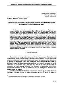
Most traditional similarity measures assume that data collections are represented as a single flat file in which each object is characterized by attributes that have a single value. However, attributes in many data sets may have multi-values, for example, the color attribute of rose can have values, {white, red}, and a person may have several salaries if he works for multiple companies. Particularly, if a data set has been extracted from several related data sets such as databases, the related information in a joined data set may have many related values for related attributes. Figure 1: (b) illustrates an example of such data sets. The data set in Figure 1: (b) can be easily created from a Personal database in (a) by joining related data sets, for example, Person data set and Purchase data set and grouping related tuples into a unique object with related values for the related attributes. In other words, the attributes, p.ptype, p.amount, and p.location are the related attributes in Purchase relation from Person relation and may have bags of values since the relationship cardinality between two relations is 1:n. A bag allows for duplicate elements unlike set but the value elements must be in the same domain. For example, the following bag {200, 200, 300, 300, 100} for the amount attribute might represent five purchases, 100, 200, 200, 300 and 300 dollars by a person. We call such a data set in Figure 1: (b) as an extended data set. We use curly bracket to represent a bag of values with the cardinality of the bag greater than one (e.g., {1,2,3}), we use null to denote an empty bag, and we just give its element, if the bag has a single value. Most traditional similarity measures for single-valued attributes can not deal with multi-valued attributes. Measuring similarity of bag of values requires group similarity measures. For example, how do we compute

ssn

43 M 21 F 67 M 35 F

(a)

location ptype amount date

111111111 Warehouse 111111111 Grocery 111111111 Mall 222222222 Mall 222222222 Grocery 333333333 Mall

1 2 3 2 3 1

400 70 200 300 100 30

02-10-96 05-14-96 12-24-96 12-23-96 06-22-96 11-05-96

ptype (payment type): 1 for cash, 2 for credit, and 3 for check, the cardinality ratio between two relations is 1:n

(b) an extended data set name age sex Johny 43 M Andy 21 F Post 67 M Jenny 35 F

p.ptype {1,2,3} {2,3} 1 null

p.amount {400,70,200} {300,100} 30 null

p.location {Mall, Grocery, Warehouse} {Mall, Grocery} Mall null

Figure 1: (a) an example of Personal relational database (b) a joined table with bags of values The problem of this approach is that by applying the aggregate function frequently valuable information may be lost (e.g., how many purchases a person has made, or how much a person has spent). In other words, this approach does not consider the cardinality information and quantitative information in computing similarity. Moreover, using aggregate functions for nominal attributes does not make sense at all, and many cases, symbolic categories are used for nominal values. The main idea of our approach is not to force the data analyst to convert sets and bags into single values, but rather to generalize existing similarity measures or clustering techniques so that they can cope with sets and bags, in addition to a single value.

2

Similarity Measures for Set or Bag of Values

There are many similarity metrics and concepts proposed in the literature from variety of disciplines in the past. For example, metric based measures are usually from engineering or science areas [1,4,6] and psychological similarity concepts and measures [2,10] are from mainly psychology area. They have their own features and useful applications, specifically depending on attribute types.

Types of attributes can be classified in different ways [1,6]. In this paper, we broadly categorize types of attributes into quantitative type and qualitative type, and introduce existing similarity measures based on these two types, and generalize those to cope with extended data sets. 2.1 Single-valued similarity measures For quantitative type of attributes, a class of distance functions known as Minkowski metric is the most popularly used dissimilarity function between two objects m

and is defined as follows: dr(a,b) = ( ∑ a i − bi r)1/r, r ≥ i =1

1, where a and b are two objects in a m-dimensional space (e.g., m number of attributes). For r = 2, it is the m

2 1/ 2

Euclidean metric, dr(a,b) = ( ∑ ( a i − bi ) ) i =1

, for r = 1,

it is the city-block (also known as taxicab or Manhattan) m

metric, dr(a,b) = ( ∑ a i − bi ) , and for r = ∞, it is the i =1

dominance metric, d∞(a,b) = max a i − bi . Euclidean 1≤ i ≤ m

distance is the most commonly used function of the Minkowski metrics. Euclidean distance is also known as the geometric invariance to translations and rotations of the object space. However, Euclidean distance assumes that the feature values in an object are not correlated with one another [6]. In many applications this assumption may not be justified. The squared Mahalanobis distance [4,6] can be used as an alternative, which for two objects ai and bi, the distance is given by di = (ai – bi )Tℑ-1(ai – bi). The matrix ℑ is usually taken to be the pooled sample covariance matrix. The Mahalanobis distance incorporates the correlation between features and standardizes each feature to zero mean and unit variance. For qualitative type of attributes, two coefficients, Matching coefficient and Jaccard’s coefficient, which are based on binary features, are the most commonly used measures. In these measures, features are assumed to have only binary values (e.g., either 0 or 1). Matching coefficient is the ratio of the number of features on which the two objects match, to the total number of features. Jaccard’s coefficient is the matching coefficient excluded the negative match. For example, let m be the total number of features, m11 be the number of features where both objects have 1 values, m00 be the number of features where both objects have 0 values, m01 be the number of features where the first object has 0 and the other one has 1, and m10 be the reverse case of m01. Then, Matching coefficient and Jaccard’s coefficient are defined as (m00+m11)/m and m11/(m−m00) respectively. There can be other varied coefficients giving weight to either matching features or mismatching features depending on the accepted practice. Here, the measure of matching features, m00 and m11 represent the number of common features and mismatching features, m01 and m10 correspond to distinctive features between two objects.

2.2 Group similarity measures 2.2.1 Qualitative type Restle [8] have investigated the concepts of distance and ordering on sets. There are several other set-theoretical models of similarity proposed [3,11]. Tversky [11] proposed his contrast model and ratio model that generalizes several set-theoretical similarity models proposed at that time. Tversky considers objects as sets of features instead of geometric points in a metric space. To illustrate his models, let a and b be two objects, and A and B denote the sets of features associated with the objects a and b respectively. Tversky proposed the following family of similarity measures, called the contrast model: S(a,b) = θf(A∩B) − αf(A − B) − βf(B − A), for some θ, α, β ≥ 0; f is usually the cardinality of the set. Here, A∩B represents the features that are common to both a and b; A − B, the features that belong to a but not to b; B − A, the features that belong to b but not to a. In the previous models, the similarity between objects was determined only by their common features, or only by their distinctive features. In the contrast model, the similarity of a pair of objects is expressed as a linear combination of the measures of the common and the distinctive features. The contrast model expresses similarity between objects as a weighted difference of the measures for their common and distinctive features. The following family of similarity measures represents the ratio model: S(a,b) = f(A∩B) / [( A∩B) + αf(A − B) + βf(B − A)], α, β ≥ 0.

In the ratio model, the similarity value is normalized to a value range of 0 and 1. The ratio model generalizes a wide variety of similarity models that are based on the Matching coefficients for binary or nominal attribute types as well as several other set-theoretical models of similarity. For example, if α = β = 1, S(a,b) becomes the Matching coefficient, f(A∩B)/(A∪B), discussed in section 2.1. If α = β = 1/2, S(a,b) becomes 2f(A∩B)/ f(A) + f(B) [3]. In Tversky’s set theoretic similarity models, a feature usually denotes a value of a binary attribute or a nominal attribute but it can be extended to interval or ordinal type. Note that the set in Tversky’s model means crisp set. Santini et al. [9] discuss the fuzzy set similarity, and extend Tversky’s model to fuzzy feature contrast model for their applications for image database. For the qualitative type of multi-valued case, Tversky’s set similarity can be used since we can consider this case as an attribute for an object has group feature values. 2.2.2 Quantitative type One simple way to measure inter-group distance is to substitute group means for the ith attribute of an object in the formulae for inter-object measures such as Euclidean distance, city-block distance, or squared Mahalanobis [4]. For example, suppose group A has mean vector A = [ x a1, x a2, …, x am] and group B has mean vector B = [ x b1, x b2, …, x bm], then the measure by Euclidean

distance between the two groups can be defined as d(A,B) m

= (

∑(x

ai

− x bi ) 2 ) 1 / 2 . The main problem of this

i =1

group mean approach is that it does not consider cardinality of quantitative elements in a group. The other way is to measure the distance between their closest or furthest members, one from each group, which are known as nearest-neighbor or furthest neighbor distance. These approaches are also used in hierarchical clustering algorithms such as single-linkage and complete-linkage [4]. The problem of this approach is that the similarity is insensitive to the quantitative variance as well as it does not account for the cardinality of elements in a group. Another approach, known as group average, can be used to measure inter-group similarity. In this approach, the between group similarity is measured by taking the average of all the inter-object measures for those pairs of objects from which each object of a pair is in different groups. For example, the average dissimilarity between n

group A and B can be defined as d(A,B) = ∑ d ( a , b ) i n , i =1

where n is the total number of object-pairs, d(a,b)i is the dissimilarity measure for the ith pair of objects a and b, a ∈ A, b ∈ B. In computing group similarity based on group average, decision on whether we compute the average for every possible pair of similarity or the average for a subset of possible pairs of similarity may be required. For example, suppose we have a pair of value set: {20,5}:{4,15} and use the city block measure as a distance function. One way to compute a group average for this pair of value set is to compute from every possible pairs, (|20-4|+|20-15|+|5-4|+|5-15|)/4, and the other way may be to compute only from corresponding pair of distance (|5-4|+|20-15|)/2 after sorting each value set. In the latter approach, sorting may help reducing unnecessary computation although it requires additional sorting time. For example, the total difference of every possible pair for value sets, {2,5} and {6,3} is 8, and the sorted individual value difference for the same set, {2,5} and {3,6} is 2. The example shows that computing similarity after sorting the value sets may result in better similarity index between multi-valued objects. We call the former one as every-pair approach, and the latter one as sorted-pair approach. This group average approach considers both cardinality and quantitative variance of elements in a group in computing similarity between two groups of values. Lance and Williams [7] point out that the average for similarity coefficients is not always acceptable and suggest a more satisfactory inter-group similarity measure than group average as follow: 1 −1 S(A,B) = cos [ cos s ( a i , b j ) ], ∑ n1 n 2 a i ∈ A,b j ∈B where S(A,B) is the similarity between groups A and B, n1 and n2 are the numbers of objects in these groups, and

s(ai ,bj) represents a single inter-object similarity measure between ai and bj, and ai ∈ A, bj ∈ B. There can be several other variations other than those methods we discussed in the above.

3

A unified similarity framework

A similarity measure proposed by Gower [5] is particularly useful for such data sets that contain a variety of attribute types. It is defined as: m

m

i =1

i =1

S(a,b) = ∑ w i s i ( a i , bi ) / ∑ w i In this formula, s(ai,bi ) is the normalized similarity index in the range of 0 and 1 between the objects a and b as measured by the function si for ith attribute and wi is a weight for the ith attribute. For example, the similarity index, s(ai,bi) can be either 1 or 0 for the qualitative type and can be a value in the range of 0 and 1 for the quantitative type. The weight wi can be also used as a mask depending on the validity of the similarity comparison on the ith attribute for a pair of objects. For example, zero is assigned to wi when the value of the ith attribute is unknown or not relevant for similarity computation for one or both objects, or when it is required to ignore the negative matches in the binary attribute. We can extend Gower’s similarity function to measure similarity for extended data sets with mixedtypes. The similarity function can consist of two subfunctions, similarity for l number of qualitative attributes and similarity for q number of quantitative attributes. We assume each attribute has the type information since data analyst can easily provide the type information for attributes. The following formula represents the extended similarity function: S(a,b) = l

q

l

q

i =1

j =1

i =1

j =1

[ ∑ w i s l ( a i , bi ) + ∑ w j s q ( a j , b j )]/( ∑ wi + ∑ w j ) , where m = l + q. The functions, sl(a,b) and sq(a,b) are similarity functions for qualitative attributes and quantitative attributes respectively. For each type of similarity measures, user makes the choice of specific similarity measures and proper weights based on attribute types and applications. For example, for the similarity function, sl(a,b), we can use the Tversky’s set similarity measure for the l number of qualitative attributes. Note that Tversky’s set similarity is a superset of the simple matching coefficient. For the similarity function, sq(a,b), we can use the group similarity function for the q number of quantitative attributes. The quantitative type of multivalued objects has additional property, group feature property including cardinality information as well as quantitative property. Therefore, sq(a,b) may consist of two sub-functions to measure group features and group quantity, sq(a,b) = sl(a,b) + sg(a,b), where the functions sl(a,b) and sg(a,b) can be Tversky’s set similarity and group average similarity functions respectively. The main objective of using Tversky’s set similarity here is to give more weights to the common features for a pair of objects.

4

An Example of Similarity Measures

Now let us illustrate an example to show how similarity between objects with bags of values can be computed. In this example, we follow the framework to compute similarity between a pair of objects in the extended data set in Figure 1. For the type information, we know that in the data set, the attributes, name, sex, ptype, and location are qualitative types, the attributes, age and amount are quantitative types. Suppose we choose the weight of each attribute as the vector, W = [0,1,1,1,1,1], then corresponding values are assigned to the attributes, name, age, sex, ptype, amount, location respectively. Note that the weight zero is assigned to the name attribute since we are not interested in the similarity of person's name. For the similarity measures, let us choose Tversky’s ratio model for qualitative attributes and city-block for quantitative attributes, for example, sl(a,b) = f(a∩b)/[( a∩b) + αf(a − b) + βf(b − a)], m

α, β = 1, and sq(a,b) = ∑ ai − bi i =1

In this example, to calculate the group similarity for quantitative attributes with a bag of values, we use sorted-pair approach. Name Johny Andy Post Jenny

Johny 0.51 0.55 0.18

Andy 0.51 0.27 0.36

Post 0.55 0.27 0.10

Jenny 0.18 0.36 0.10 -

Table 4.1: A similarity table for Figure 1: (b) using weights W = [0,1,1,1,1,1], |W| = 5 The table 4.1 summarizes the normalized similarity index by objects when the weight for each attribute is given as a unit vector which assigns the same degree of significance to every attribute, except for the attribute name. The scalar value of the weight vector W (i.e., |W| = 5) is used to normalize the similarity index in the range of 0 and 1. In this table, we can easily recognize which object is closer to which object than the other objects. For example, the object “Johny” is more similar to “Post” than “Andy” and more similar to “Andy” than “Jenny” in the given data set. Name Johny Andy Post Jenny

Johny 0.58 0.47 0.14

Andy 0.58 0.29 0.20

Post 0.47 0.29 0.08

Jenny 0.14 0.20 0.08 -

Table 4.2: A similarity table for Figure 1: (b) using weights W = [0,1,0.5,2,2,1], |W| = 6.5 The similarity index in the Table 4.1 also shows that decision on weights for attributes may affect the similarity significantly. For example, the similarity index for the object pair (Johny,Post) is higher than the pair (Johny,Andy), mainly because of the matching attribute sex although “Johny” has more common features to “Andy” than “Post” in other attributes ptype, amount, and

location. We can show this fact by assigning different weights to attributes in computing similarity. For example, suppose the weight vector is now [0,1,0.5,2,2,1] by assigning more significance to attributes ptype and amount and less significance to the attribute sex, then we can have different similarity index table in Table 4.2, which shows different similarity relationships between objects. The similarity index table in Table 4.2 shows that “Johny” is more similar to “Andy” than “Post” unlike the similarity index in Table 4.1 because the matching attribute sex does not affect very much this time. Therefore, user’s experience and knowledge about the given data set is important for selecting proper weights for attributes. To help user decide proper weights, using statistical information, such as correlation coefficients or regression analysis, may be helpful to assist the user in selecting the proper weight.

5

Summary

We discussed various families of similarity measures for single-valued attributes and group similarity measures. Then, we proposed a unified framework for similarity measures to cope with mixed-type attributes that may have set or bag of values. Our unified similarity function is a function that combines the several existing similarity measures based on multiple data types. We also gave an example based on the proposed similarity framework. We are currently in the process of generalizing and experimenting with clustering algorithms such as Nearest-neighbor algorithm, hierarchical clustering, and K-means based on the proposed similarity framework for clustering extended data sets.

References Anderberg, M.R. Cluster analysis for application. New York, NY: Academic Press, 1973. [2] Ashby, F.G. and Perrin, N.A. Toward a unified theory of similarity and recognition. Psychological review, 95(1): 124-150, 1988. [3] Eisler, H. and Ekman, G. A mechanisim of subjective similarity. Acta Psychologica, 1959. [4] Everitt, B.S. Cluster Analysis. Edward Arnold, Copublished by Halsted Press and imprint of John Wiley & Sons Inc., 3rd edition, 1993. [5] Gower, J.C. A general coefficient of similarity and some of its properties. Biometrics 27, 857-872. 1971. [6] Jain, A.K, and Dubes, R.C. Algorithms for clustering data, Englewood Cliffs, NJ: Prentice Hall, 1988. [7] Lance, G.N. and Williams, W.T. A general theory of classificatory sorting strategies: I. Hierarchical systems. Computer Journal 9, 373-380, 1967. [8] Restle, F. A metric and an ordering on sets. Psychometrika, 24, 207-220, 1959. [9] Santini, S. and Jain, R. Similarity Queries in Image Databases. Proc. of IEEE Conference on Computer vision and Pattern recognition, 1996. [10] Shepard, R.N. The analysis of proximities: Multidimensional scaling with unknown distance function. Part I. Psychometrika, 27:125-140, 1962. [11] Tversky, A. Features of similarity. Psychological review, 84(4): 327-352, July 1977.

[1]