A Unifying Framework for Devising Efficient and Irreversible MCMC ...

arXiv:1608.05973v1 [stat.ME] 21 Aug 2016

A Unifying Framework for Devising Efficient and Irreversible MCMC Samplers Yi-An Ma1 , Tianqi Chen2 , Lei Wu3 , and Emily B. Fox4 1

2

Department of Applied Mathematics, University of Washington Department of Computer Science and Engineering, University of Washington 3 School of Mathematical Sciences, Peking University 4 Department of Statistics, University of Washington August 23, 2016 Abstract

We propose a framework for Markov chain Monte Carlo using both continuous dynamics and jump processes that enable the development of efficient, irreversible samplers. For each component, we decompose the dynamics into reversible and irreversible processes, and with a parameterization that is easy to specify while ensuring the correct stationary distribution. For the continuous dynamic samplers, we prove that all such samplers can be encoded by a positive semidefinite diffusion matrix D and skew-symmetric curl matrix Q, where D determines the reversible part and Q drives the irreversible process. Using our proposed parameterization, it is straightforward to ensure that the target distribution is preserved. We likewise discuss scalable variants using stochastic gradients for large-scale Bayesian inference, and use our framework to propose a Riemann version of stochastic gradient Hamiltonian Monte Carlo. For samplers following jump processes, we prove that such samplers can be represented by a symmetric kernel S and an anti-symmetric kernel A, with straightforward conditions to satisfy to preserve the target distribution. Paralleling the continuous framework, S determines the reversible part and A the irreversible process. As a practical algorithm, we propose an implementation akin to Metropolis Hastings—with the same ease and efficiency—but allowing for irreversible dynamics. In our experiments, we demonstrate the benefits of such irreversibility across a broad range of target distributions. Finally, we combine the frameworks and show how one can use the continuous dynamics as a proposal distribution in the irreversible jump sampler. This can be viewed either as a method for correcting for bias in the discretized continuous dynamics or as a method for incorporating geometric information into the irreversible jump sampler.

1 Introduction Markov chain Monte Carlo (MCMC) methods are the defacto tools for inference in Bayesian models. There are two primary approaches to developing and implementing such MCMC algorithms. One is the traditional MetropolisHastings type of approach, where one defines a jump process through an accept-reject procedure. This popular class of methods utilizes global information of the target distribution. Another approach relies on the local (gradient) information of the target distribution and designs a continuous dynamical process with the target distribution as its stationary distribution; samples are proposed according to the integrated trajectories of the continuous dynamics. Important examples of such samplers include Hamiltonian Monte Carlo methods [15, 28] and samplers using Langevin dynamics [31, 38, 36, 29].

1

For both approaches, a major challenge is devising a sampler with good mixing rates (i.e., the speed at which an initial distribution converges to the target distribution). In the world of jump process based MCMC techniques, a focus has been on developing clever proposals [32, 20], but these methods are often strongly coupled to a specific challenge setting, like multimodal targets [32] or heavy tailed distributions [20]; in practice, one often does not know the structure of the target distribution, which might additionally exhibit a combination of these factors. In the world of continuous-dynamic-based samplers, methods using second order information, like Riemannian Hamiltonian Monte Carlo [17], can be helpful. However, it is non-trivial to devise these modifications and prove that the dynamics maintain the right stationary distribution. In this paper, we propose a unifying framework for these two approaches that enables a more user-friendly method for devising efficient and general-purpose MCMC procedures. We start by examining continuous dynamic samplers. We present a stochastic differential equation (SDE) based framework in which to define all such valid samplers based on specifying two matrices: a positive semidefinite diffusion matrix and a skew-symmetric curl matrix. These matrices define symmetric (reversible) and anti-symmetric (irreversible) operators, respectively. Based on this framework, we prove that for any choice of these matrices, the sampler will have the target distribution as the stationary distribution. We likewise prove that any continuous dynamic sampler with the correct stationary distribution has a representation in this framework. As such, we call this framework complete. We cast a number of past methods in our proposed representation, and also show how it can be used to devise new samplers with improved mixing rates. An initial version of this work appeared in [24]. In [24], jump processes were specifically excluded from the analysis. However, jump processes represent a potentially attractive approach to MCMC since, in theory, samples generated from jump processes can decorrelate rapidly. In practice, it is challenging to define transition kernels that enable this efficient exploration while maintaining a reasonably high acceptance rate. The challenge partially stems from the fact that attention has typically been restricted to reversible jump processes. Such samplers are straightforward to derive and implement, but the reversibility restriction hinders the mixing rates and efficiency of the proposed algorithms [27, 13, 11, 9]. Unfortunately, devising irreversible samplers is a non-trivial task, and often results in computationally complex algorithms. Leveraging our insights from the operator decomposition for continuous dynamic processes, we show that a similar framework can enable the development of efficient irreversible jump process samplers based on the specification of two kernel functions. We decompose the jump operator into symmetric (reversible) and anti-symmetric (irreversible) operators, paralleling the continuous-dynamic sampler framework. Using this decomposition and parameterization, we arise at a straightforward set of constraints on the transition kernels that ensures that the target distribution is the stationary distribution. The resulting sampler implementation has the ease and efficiency of Metropolis-Hastings; in fact, the implementation directly parallels that of standard Metropolis-Hastings. In terms of runtime, our proposed methods significantly outperform previous approaches [26, 19], in addition to providing fast mixing rates in a range of scenarios, from heavy-tailed to multimodal targets. We demonstrate these performance gains against existing approaches in a variety of sampling tasks. There are many ways we can think of combining our continuous dynamic and jump process frameworks. One is to use the continuous dynamic sampler and jump process sampler iteratively, i.e., use one (possibly for multiple iterations) and then the other, just as in Hamiltonian Monte Carlo. Another approach is to use the continuous dynamic sampler for some variables (e.g., real-valued variables) and the jump process sampler for others (e.g., discrete-valued variables). It is straightforward to combine our approaches in these manners since each process maintains the correct stationary distribution, so these types of compositions will likewise result in the correct stationary distribution under some mild conditions at stationary. Alternatively, as we show, we are able to use the continuous dynamics as a proposal distribution in our jump process accept-reject scheme, even when the continuous dynamics are not reversible. Here, the transition kernel is defined by simulating the discretized SDE associated with the continuous dynamics. We can view the benefits of this approach from two angles: (i) the SDE can provide an efficient proposal distribution for our irreversible Markov jump process or (ii) the accept-reject scheme allows us to correct for the bias introduced by sampling the

2

continuous dynamics via a discretized SDE. This accept-reject scheme is a direct generalization of the Metropolis adjusted Langevin algorithm (MALA) [31] to irreversible SDEs. This opens up the possibility to combine, for example, the benefits of Langevin diffusion with Hamiltonian dynamics. As we see, combining our frameworks for continuous dynamic processes and Markov jump processes yields a unified and complete framework for devising efficient and general purpose MCMC samplers with the correct stationary distribution. Another important challenge of MCMC in practice is scaling such approaches to large datasets. In these cases, calculating the necessary likelihood term (or its gradient) at every MCMC step can be computationally prohibitive. In Section 7, we discuss and devise minibatch based alternatives that only rely on a randomly selected subset of the data per iteration. The result is a highly scalable recipe for MCMC, capturing many previously proposed approaches [36, 10, 29, 14]. We illustrate the utility of this framework by proposing a Riemann variant of stochastic gradient Hamiltonian Monte Carlo; we demonstrate its improvement over a number of baselines in a streaming analysis of Wikipedia articles.

2 Background We start with the standard MCMC goal of drawing samples from a target distribution π(z). The idea behind MCMC is to translate the task of sampling from the posterior distribution to simulating from a Markov process. One can then discuss the evolution of the distribution p(z; t) under this stochastic process and analyze its stationary distribution, ps (z). If the stochastic process is ergodic and its stationary distribution is equal to the target distribution π(z), then simulating the stationary stochastic dynamics equates with providing samples from the posterior distribution. In this section, we review some of the fundamentals of the stochastic processes associated with general Markov processes, and how we can use these processes to construct samplers.

2.1 General Markov Processes and their Diffusion and Jump Operators Consider a general Markov process in Rd , described by the Chapman-Kolmogorov (CK) equation: Z p(z|x; t1 + t2 ) = dyp(z|y; t2 )p(y|x; t1 ),

(1)

Rd

where t1 < t2 are two arbitrary scalar variables denoting time and x, y, z ∈ Rd . For succinctness of presentation, we let p(y|x; t) denote the probability of transition from x to y over time t and use autonomous Markov processes (i.e., with time invariant Markov transition operators). However, it is worth noting that the autonomous assumption is not necessary to any of the calculations and that non-autonomous Markov processes bear exactly the same results. A differential form of Eq. (1), from which algorithms are more straightforwardly derived, can be obtained by assuming three mild existence conditions specified in Appendix A.1. The differential CK equation defines an update rule that consists of a diffusion process and a jump process: d d X  X  ∂2  ∂  ∂ p(z|y; t) = Dij (z)p(z|y; t) − fi (z)p(z|y; t) ∂t ∂zi ∂zj ∂zi i,j=1 i=1 Z h i dx W (z|x)p(x|y; t) − W (x|z)p(x|z; t) . +

(2)

Rd

Here, f is any real-valued function, W is a transition kernel, and D is a d × d positive semidefinite matrix. The first line denotes a continuous Markov process specified by a Fokker-Planck operator on p(z|y; t); the second line is a jump process defined by the transition kernel W (z|x).

3

In this paper, we rewrite Eq. (2) as (assuming that the target distribution π(z) is the stationary distribution for both the Fokker-Plank equation and the Markov jump process)     ∂ p(z|y; t) p(z|y; t) b b +J , (3) p(z|y; t) = L ∂t π(z) π(z)

b is a diffusion operator defined as: where L[·]

Lb [ϕ(z)] =

d X

i,j=1

n X ∂2 ∂ [Dij (z)π(z)ϕ(z)] − [fi (z)π(z)ϕ(z)] , ∂zi ∂zj ∂z i i=1

and Jb[·] is a Markov transition (jump) operator with kernel W (z|x): Z dx [W (z|x)π(x)ϕ(x) − W (x|z)π(z)ϕ(z)] . Jb [ϕ(z)] =

(4)

(5)

Rd

This form allows us to do two things straightforwardly: One is to separate our analyses of the continuous and jump parts; the second is to analyze the reversibility of the processes. In particular, reversible processes satisfy the p(x|y; t) p(y|x; t) algebraic condition that = , or as is more commonly written, p(x|y; t)π(y) = p(y|x; t)π(x). π(x) π(y) When the operators Lb and Jb on p(z|y; t)/π(z) are self-adjoint (i.e., their adjoint operators in the Hilbert space are equal to themselves), the Markov process is reversible. Hence, expressing the evolution of the current probability distribution with respect to the stationary distribution as in Eq. (3) can help reveal this structure. For simplicity, to ensure the correctness of the resulting samplers, in this paper we assume that individually the continuous and jump Markov processes each have π(z) as their invariant solution (i.e., π(z) is in the null space of both operators). Thus, when combined, π(z) will be the invariant solution of the combined operator of Eq. (3).

2.2 Constructing Samplers from Continuous and Jump Markov Processes In Section 2.1, we described the evolution of the distribution p(z|y; t). This evolution provides insight into the stationary distribution of the process. Here, we present the dynamics for an individual realization, which will play a critical role in our developed samplers.   p(z|y; t) ∂ , can be generated from the p(z|y; t) = Lb A realization of the continuous Markov process, ∂t π(z) stochastic differential equation (SDE): p dz = f (z)dt + 2D(z)dW(t). (6) In practice, to simulate from Eq. (6), we consider an ǫ-discretization:

zt+1 ← zt + ǫt f (zt ) + N (2ǫt D(zt )).

(7)

Although Eq. (7) is in the form of the Euler–Maruyama method, higher order numerical schemes can be used for better accuracy [8, 7, 23]. The challenge here is to select f and D such that Eq. (4) has the right stationary distribution, implying that the simulation from Eq. (6) provides samples from π(z). Note that relying on a sample path from the discretized system of Eq. (7) typically leads to the introduction of bias due to discretization error. In these cases, the samples only provide unbiased estimates in the limit as ǫt → 0 unless further corrections are introduced. In Section 3, we propose a reparameterization of Eq. (6) from which it is trivial to ensure the SDE has the desired stationary distribution. Then, in Section 5, we return to the idea of correcting for any potential discretization error if no bias can be tolerated. 4

Turning to the jump Markov process, the equation order in ∆t given by: p(z|y; t + ∆t) = ∆t

Z

Rd

  ∂ p(z|y; t) is approximately to the first p(z|y; t) = Jb ∂t π(z)

 Z W (x|y)p(x|y; t)dx + 1 − ∆t

Rd

 W (x|y)dx p(z|y; t).

(8)

Although this is an approximation to the original equation, it has the same stationary distribution. Noting that p(x|y; 0) = δ(z − y), we arise at the transition probability:   Z W (x|y)dx δ(z − y). (9) p(z|y; ∆t) = ∆tW (z|y) + 1 − ∆t Rd

Eq. (9) corresponds to a sampling process as follows. We take ∆t to R be the stepsize. Then, with probability ∆tW (z|y), we transit from state y to state z. With probability 1 − ∆t Rd W (x|y)dx, we stay in state y. Analogously to the challenge of selecting f and D, the challenge here is to select the kernel W (z|x) that leads to the stationary distribution being equal to the target distribution, π(z). This requires that the positive transition R kernel W satisfies Rd dx [W (z|x)π(x) − W (x|z)π(z)] = 0. Additionally, even if such a W can be defined, it might not define a distribution from which we can straightforwardly sample nor compute the necessary integral. Instead, in practice one typically resorts to implementing jump process samplers through the Metropolis-Hastings (MH) accept-reject scheme [26, 19]. In MH (Algorithm 1), one samples from a specified proposal distribution q(z|y) and accepts the proposed value z with probability   π(z)q(y|z) . (10) α(y, z) = min 1, π(y)q(z|y) In the form of Eq. (9), we have [12]:  Z p(z|y; ∆t) = q(z|y)α(y, z) + 1 −

Rd

 q(x|y)α(y, x)dx δ(z − y).

(11)

When in state y at time t, we propose to jump to state z at t + ∆t with conditional probability q(z|y), realized via a random number generator that has a distribution according to q(z|y); we accept this proposal with probability α(y, z) to ensure that the target distribution will be preserved under this procedure. Hence, the total probability of transiting from state y to z is q(z|y)α(y, z). Otherwise, we stay in state y. Comparing to Eq. (9), we see that MH restricts our attention to W (z|y) satisfying ∆tW (z|y) = q(z|y)α(y, z). We further see that the acceptance R rate α(y, z) is specifically designed so that W (z|x)π(x) = W (x|z)π(z), a condition much stronger than Rd dx [W (z|x)π(x) − W (x|z)π(z)] = 0, implying that π(z) is the stationary distribution. However, this form restricts our attention solely to reversible processes. Instead, just as in the continuous Markov process case, in Section 4 we consider a reparameterization in terms of two kernel functions with straightforward-to-satisfy constraints. In that form, not only do we ensure the right stationary distribution, but we are able to devise a sampling algorithm for irreversible processes that has the same simplicity of implementation as MH. Taken together, the results of Sections 3 and 4 alluded to in this section imply that by simply specifying two matrices and two modestly constrained kernel functions, one can devise samplers where we know both the continuous and jump components will have the right stationary distribution. We can compose these two processes in various ways and still ensure that the overall sampler has the correct stationary distribution as is discussed in Section 5.

5

Algorithm 1: Metropolis-Hastings Algorithm for t = 0, 1, 2 · · · do sample u ∼ U[0,1] propose z(∗) ∼ q(z(∗)|z(t))  
π (z(∗)) q(z(t)|z(∗)) (t) α z , z(∗) = min 1, π (z(t)) q(z(∗)|z(t)) if u < α (z(t), z(∗)), z(t + 1) = z(∗) else z(t + 1) = z(t) end

3 Continuous Markov Process Based Samplers b in Eq. (4) and We start by examining how to use continuous processes—described by the diffusion operator L[·] realized by the SDE in Eq. (6)—to construct samplers. Although Eq. (6) provides a way to simulate the continuous dynamics and obtain samples from the Markov process, it is not clear which choice of f and D will result in a stationary distribution equal to the target distribution from which we wish to sample. For a given f and D, Eq. (4) allows us to analyze this stationary distribution, but it is very challenging to construct f and D to yield a specified stationary distribution. Instead, we propose to use an alternative form for the diffusion operator specified via two matrices D and Q, as well as the target distribution π(z):     T L [ϕ(z)] = ∇ · D(z) + Q(z) [(∇ϕ(z)) π(z)] . (12)

Here, D(z) is a positive semidefinitediffusion matrix and  Q(z) a skew-symmetric matrix. An element–wise   d   P ∂ϕ(z) ∂ π(z) . For this representation to be Dij (z) + Qij (z) representation of L [ϕ(z)] is: ∂zj i,j=1 ∂zi useful, we need to verify two properties: One is that L[·] has π(z) as its invariant distribution; the other is that any process with π(z) as the invariant distribution can be written in the form of Eq. (12) (i.e., there exists a D(z) and Q(z) that place the process in this representation). Together, these two properties would (i) allow us to very straightforwardly explore a set of valid samplers by specifying pairs (D(z), Q(z)) of positive semidefinite and skew-symmetric matrices, respectively, and (ii) ensure that as we span the space of all possible (D(z), Q(z)), we know we have covered all possible valid samplers. That is, we would say our representation was complete.   ∂p(z|y; t) p(z|y; t) s It is straightforward to verify that p (z) ∝ π(z) is a stationary solution to the equation =L ∂t π(z) with L[·] as in Eq. (12). More significantly, Theorem 1 states that any process with stationary distribution π(z) has a representation in our framework.   ∂p(z|y; t) p(z|y; t) b as in Eq. (4) has stationary probability density function for L[·] = Lb Theorem 1. Suppose ∂t  π(z)  Pd ∂  s s s Dij (z)p (z) is integrable with respect to the p (z) ∝ π(z). Further assume that fi (z)p (z) − j=1 ∂θj b is Lebesgue measure. Then, there exists a skew-symmetric matrix Q(z) such that the diffusion operator L[·] equivalent to the operator L[·] in Eq. (12). We give a constructive proof of Theorem 1 in Appendix B. The equivalence between L [·] and Lb [·] arises by taking f (z) = −[D(z) + Q(z)]∇H(z) + Γ(z), 6

for H(z) = − log(π(z)) and Γi (z) =

Pd

j=1


∂ Dij (z) + Qij (z) . Hence, the SDE realization of the Markov ∂zj

processes following the new L operator is h i p
dz = − D(z) + Q(z) ∇H(z) + Γ(z) dt + 2D(z)dW(t).

(13)

3.1 Decomposing L[·] into Reversible and Irreversible Dynamics The operator L[·] can be decomposed into a symmetric part LS [·], characterizing a reversible Markov process, and an anti-symmetric part LA [·], representing an irreversible process. The symmetric and skew-symmetric operators corresponds to two different kinds of dynamics. The symmetric operator is determined solely by the diffusion matrix D since the skew-symmetric matrix Q cancels out:        p(z|y; t) p(z|y; t) 1 p(z|y; t) LS = L + L∗ π(z) 2 π(z) π(z)  !   p(z|y; t) T π(z) =∇ · D(z) ∇ π(z)   d X ∂2 Dij (z)p(z|y; t) = ∂zi ∂zj i,j=1    d X ∂ X ∂H(z)  . Dij (z) + − ΓD (14) i (z) p(z|y; t) ∂z ∂z i j i=1 j Pd

∂ Dij (z) and L∗ [·] denotes the adjoint operator of L[·]. According to Itˆo’s convention, the ∂zj   p(z|y; t) ∂ corresponds to reversible Brownian motion in last two lines of Eq. (14) implies that p(z|y; t) = LS ∂t π(z)  a potential force field on a Riemannian manifold specified by the diffusion matrix D(z): dz = − D(z)∇H(z) + p  ΓD (z) dt + 2D(z)dW(t). This is referred to as Riemannian Langevin dynamics [31]. When D(z) is positive definite, the reversible Markov dynamics have nice statistical regularity and will drive the system to converge to the stationary distribution. The anti-symmetric operator is dictated solely by Q, as here D cancels out:        p(z|y; t) 1 p(z|y; t) p(z|y; t) = L − L∗ LA π(z) 2 π(z) π(z)  !   p(z|y; t) T π(z) =∇ · Q(z) ∇ π(z) ! h i =∇T · Q(z)∇H(z) − ΓQ (z) p(z|y; t) . (15) Here, ΓD i (z) =

j=1

  ∂ ∂ A p(z|y; t) Here, = Qij (z). The last line of Eq. (15) demonstrates that p(z|y; t) = L j=1 ∂zj ∂t π(z) is a Liouville equation, which describes the density evolution of p(z|y; t) according to conserved, deterministic dynamics: dz/dt = −Q(z)∇H(z) + ΓQ (z), with π(z) its invariant measure. ΓQ i (z)

Pd

7

Algorithm 2: Generalized Riemann Hamiltonian Monte Carlo initialize (z) for i = 1 · · · n do for t = 0, 1, 2 · · · do P ∂ (Dij (z) + Qij (z)) Γi (z) = j ∂zj end 
 zt+1 ← zt − ǫt D(zt ) + Q(zt ) ∇H(zt ) + Γ(zt ) + N (2ǫt D(zt )) end Combining the dynamics of Eqs. (14) and (15) leads to a general SDE, Eq. (13), with stationary distribution π(z). Previous methods [31, 38, 36, 29, 28] have primarily focused on solely symmetric or anti-symmetric operators, LS or LA , respectively, as we make explicit in Section 3.3. In Section 7, we describe some samplers using both operators, but without a general procedure for constructing and analyzing such samplers.

3.2 Continuous Markov Process Sampling Algorithm Following Eq. (7), we can simulate from the SDE underlying the operator in Eq. (13) using the following ǫdiscretization: 
 (16) zt+1 ← zt − ǫt D(zt ) + Q(zt ) ∇H(zt ) + Γ(zt ) + N (2ǫt D(zt )). Again, higher-order numerical schemes can be used in place of the first-order integrator above [8, 7, 23]. The resulting algorithm is outlined in Algorithm 2. (Recall that bias is introduced via the discretization, i.e., setting ǫt finite. We will return to this in Section 5.)

3.3 Previous MCMC Algorithms as Special Cases We explicitly state how some previous continuous-dynamic-based MCMC methods fit within the proposed framework based on specific choices of D(z), Q(z) and H(z). We show how our framework can be used to “reinvent” the samplers by guiding their construction and avoiding potential mistakes or inefficiencies caused by na¨ıve implementations. Hamiltonian Monte Carlo (HMC) The key ingredient in HMC [15, 28] is Hamiltonian dynamics, which simulates the physical motion of an object with position θ, momentum r, and mass M on an frictionless surface as follows:  θt+1 ← θt + ǫt M−1 rt (17) rt+1 ← rt − ǫt ∇U (θt ). (Note that above we consider a straightforward integrator, whereas in practice it is common to use a leapfrog simulation instead [28].)  Eq. (17) is  a special case of the proposed framework with z = (θ, r), H(θ, r) = U (θ) + 0 −I 1 T −1 r, Q(θ, r) = and D(θ, r) = 0. 2r M I 0 Langevin Dynamics The Langevin dynamics sampler [31, 36] proposes to use the following first order (no momentum) Langevin dynamics to generate samples θt+1 ← θt − ǫt D∇U (θt ) + N (0, 2ǫt D). 8

(18)

This algorithm corresponds to taking z = θ with H(θ) = U (θ), D(θ) = D, and Q(θ) = 0. Riemannian Langevin Dynamics The Langevin dynamics sampler can be generalized to use an adaptive diffusion matrix D(θ). Specifically, it is interesting to take D(θ) = G−1 (θ), where G(θ) is the Fisher information metric [38, 29]. The sampler iterates θt+1 ← θt − ǫt [G(θt )−1 ∇U (θt ) + Γ(θt )] + N (0, 2ǫt G(θt )−1 ).

(19)

We can cast this Riemannian Langevin dynamics sampler [29] into our framework taking D(θ) = G(θ)−1 , and P ∂Dij (θ) Q(θ) = 0. From our framework, we know that here Γi (θ) = . Interestingly, in earlier literature [18], ∂θj j
P ∂ −1 Γi (θ) was taken to be 2 |G(θ)|−1/2 Gij (θ)|G(θ)|1/2 . More recently, it was found that this correction j ∂θj term corresponds to the distribution function with respect to a non-Lebesgue measure [31]. For the Lebesgue measure, the revised Γi (θ) was as determined by our framework [31]. This is an example of how our theory provides guidance in devising correct samplers. Summary of past samplers In our framework, the Langevin dynamic based samplers take Q(z) = 0 and instead stress the design of the diffusion matrix D(z). The standard Langevin dynamic sampler uses a constant D(z), whereas the Riemannian variant uses an adaptive, z-dependent diffusion matrix to better account for the geometry of the space being explored. On the other hand, HMC takes D(z) = 0 and focuses on the curl matrix Q(z). As we see, our method is a generalization of the dynamics underlying Hamiltonian Monte Carlo (and Riemannian Hamiltonian Monte Carlo) methods, extending the symplectic  structure  to be non-constant. That 0 −I is, considering general skew–symmetric matrices instead of just Q(z) = [33, 16]. The generalized I 0 Hamiltonian dynamics can explore the state space rapidly, and are guaranteed to preserve the stationary distribution once it is achieved. Examination of the past methods provides us with the insight that D(z) can enable diffusive exploration across local modes while Q(z) can enable rapid traversing of low-probability regions, especially when state adaptation is incorporated. Importantly, through our (D(z), Q(z)) parameterization, we can readily examine which parts of the product space D(z) × Q(z)—representing the space of all possible samplers—have been covered. We see that a majority of possible samplers have not yet been considered. In Section 7.1.2, we will discuss how to use the current framework to devise new samplers.

4 Samplers Using Jump Processes with Operator J [·] b We now turn our attention to the jump operator Jb[·] of Eq. (5). As with the continuous dynamic operator L[·], we can consider an equivalent representation that enables more ready analysis of the properties of the process, and the development of efficient irreversible jump process samplers. Based on the form of Eq. (9) specified by generic kernel W (x|z), it is challenging to determine which choice of W (x|z) leads to a jump process with the correct stationary distribution. Even if one can construct such a W , it can be challenging to use W to sample a realization of the jump process; instead, often one restricts attention to reversible processes and uses MH. (See Section 2.2.) We instead consider an equivalent but alternative representation defined in terms of two kernels S and A. A simple set of constraints on S and A ensures that the target distribution π(z) is the stationary distribution of the jump process.

9

In particular, we consider J [ϕ(z)] =

Z

Rd

dx




 S(x, z) + A(x, z) ϕ(z) − S(x, z)ϕ(z) ,

(20)

where S is a symmetric kernel and A is an anti-symmetric kernel. Based on the form of Eq. (20), as shown in Appendix C.1, we simply have to satisfy the following constraints in order to ensure that π(z) is the stationary distribution: R R 1. Rd S(x, z)π −1 (x)dx and Rd A(x, z)π −1 (x)dx exist 2. S(x, z) + A(x, z) > 0 R 3. Rd A(x, z)dx = 0.

Following Eq. (9), the transition probability implied by the operator of Eq. (20) assuming a ∆t-discretization is given by:   Z
∆t ∆t S(y, z) + A(y, z) + 1 − S(y, x)dx δ(z − y). (21) p(z|y; ∆t) = π(y) π(y) Rd

Since the jump operator has π(z) as the stationary distribution assuming the constraints of Eq. (3) are satisfied, then the transition probability of Eq. (21) defines a valid procedure for drawing samples from the target π(z). In particular, over time ∆t, state y transitions to state z with probability ∆t(S(y, z) + A(y, z))/π(y), and state y   ∆t R remains unchanged with probability 1 − d S(y, x)dx . In Section 4.3, we examine a practical algorithm π(y) R for efficiently implementing such a procedure based on an accept-reject scheme analogous to the MH algorithm outlined in Algorithm 1. The important challenge we conquer is handling the irreversibility of the process arising from A 6= 0. We study these irreversible dynamics in Section 4.1.

4.1 Reversible and Irreversible Dynamics of J [·] Similar to operator L[·], operator J [·] can also be decomposed into a symmetric (reversible) part J S [·] and antisymmetric (irreversible) part J A [·]: 1 J S [ϕ(z)] = (J [ϕ(z)] + J ∗ [ϕ(z)]) 2Z dx [S(x, z)ϕ(x) − S(x, z)ϕ(z)] ; =

(22)

Rd

1 J A [ϕ(z)] = (J [ϕ(z)] − J ∗ [ϕ(z)]) 2Z dx [A(x, z)ϕ(x)] . =

(23)

Rd

Here, J ∗ [·] is the adjoint operator of J [·]. We see that A fully determines the irreversible dynamics whereas S defines the reversible part. We can further derive from Eq. (21) that A is the difference between the probability of a forward path and the backward path: A(x, z) =


1 π(y)p(z|y; ∆t) − π(z)p(y|z; ∆t) . 2∆t 10

(24)

4.2 Previous Samplers as Special Cases As with past continuous-dynamic-based samplers, we now cast a set of past jump process based samplers into our framework. 1 Direct resampling Methods that sample directly from π(z) take S(y, z) = π(y)π(z) and A(y, z) = 0. We ∆t can verify this by substituting into Eq. (21). Metropolis-Hastings

The very popular MH algorithm falls into our framework taking A(y, z) = 0 and S(y, z) =


1 min π(y)q(z|y), π(z)q(y|z) . ∆t

(25)

To see this, we refer to Section 2.2. The specified form for S and A above arises from comparing the transition probability of Eq. (11) with that of Eq. (21). Summary of past samplers In the previously mentioned algorithms, and a majority of those used in practice, only reversible Markov jump processes (A(z, y) = 0) are considered. In Section 4.3, we explore the case where the process is irreversible, i.e., A(z, y) 6= 0.

4.3 Construction of Irreversible Jump Processes for MCMC Analogous to the discussion of Section 2.2, there are two issues of designing samplers with Markov jump processes. One is the construction of transition kernels, a task that has been alleviated in part by the new formulation of Eq. (21) in terms of S(y, z) and A(y, z) with simple constraints, though we still have to construct such kernels. Another is simulating the Markov process of Eq. (21). In all but the simplest cases, we might not be able to sample from the transition probability ∆t · (S(y, z) + A(y, z))/π(y). These two issues are often intertwined to pose challenges to the design of samplers. As mentioned in Section 2.2, the MH algorithm is often resorted to due to its ease of implementation. It separates the process of proposing a sample into two simple steps: (1) proposing a candidate according to a known conditional probability distribution q(z|y) and (2) accepting or rejecting the candidate according to a certain probability. An important drawback of the vanilla MH sampler, however, is that the reversibility of the jump process being designed can greatly restrict possible ways to increase the mixing of the Markov chain. There have been previous efforts to break the restriction of reversibility in different cases. For example, the “non-reversible MH” algorithm adds a vorticity function to the MH procedure to sample the multivariate Gaussian distribution [4]; the “lifting method” makes two replica of the original state space with a skew detailed balance condition to ensure that the integral of A is zero in the spin models [34, 35]; the “Zig-Zag” sampler further uses gradient information to guide the construction of the two Markov chains on the replicated space to efficiently sample in the Curie-Weiss model [5]. It is unclear how to generalize these past methods to handle a broad set of target distributions. Here, we show how we can devise a practical and efficient irreversible jump process algorithm analogous to MH that can be applied to general targets; this procedure implicitly defines valid kernels S(y, z) and A(y, z). In particular, just as MH corresponds to restricting the class of kernels W (z|y), our algorithm also focuses in on particular instances of A(y, z), but importantly allow A(y, z) 6= 0 (i.e., irreversible processes). The value of this in practice is demonstrated in the experiments of Section 6. A na¨ıve approach The most straightforward approach to devising an irreversible sampler is to utilize different proposal distributions f (z|y) and g(z|y), instead of a single q(z|y), such that the transition kernels of MH

11

Algorithm 3: One-Dimensional Irreversible Jump Sampler randomly pick z p from {1, −1} with equal probability for t = 0, 1, 2 · · · do sample u ∼ U[0,1] if z p > 0 then sample z(∗) ∼ f (z(∗)|z(t))   π (z(∗)) g (z(t)|z(∗)) α (z(t), z(∗)) = min 1, π (z(t)) f (z(∗)|z(t)) end else sample z(∗) ∼ g (z(∗)|z(t))   π (z(∗)) f (z(t)|z(∗)) α (z(t), z(∗)) = min 1, π (z(t)) g (z(∗)|z(t)) end if u < α (z(t), z(∗)), z(t + 1) = z(∗); z p (t + 1) = z p (t) else z(t + 1) = z(t); z p (t + 1) = −z p (t) end

algorithm in Eq. (25) is changed to F (y, z) = S(y, z) + A(y, z) =


1 min π(y)f (z|y), π(z)g(y|z) . ∆t

(26)


1 Here we are considering jump processes with A(y, z) = F (y, z) − F (z, y) 6= 0, in contrast to what we saw 2 for MH. By adjusting f and g, faster mixing rates can possibly be attained while maintaining a simple sampling and g in place of q in the procedure akin to that of MH (see Algorithm 1, but with f in place of q in the numerator R denominator in the α calculation). The primary issue with this construction is that Rd A(y, z)dy 6= 0 in general, rendering the stationary distribution not the π(z) that we desire. The question is how to design the anti-symmetric R kernel A(y, z), such that Rd A(y, z)dy = 0.

Lifting for sampling when d = 1 A simple modified approach is to follow an adjoint Markov process after being rejected by the original one. This is inspired by the “lifting” idea in discrete spaces [34, 35]. Importantly, this approach has π(z) as the stationary distribution. Algorithmically, this process introduces a one-dimensional, uniformly distributed discrete auxiliary variable yp ∈ {−1, 1}. We then define
fe(z, zp |y, yp ) = H(yp )f (z|y) + H(−yp )g(z|y)
ge(z, zp |y, yp ) = H(−yp )f (z|y) + H(yp )g(z|y) ,

(27)

where f (z|y) and g(z|y) are different conditional probability distributions, and H is the Heaviside function:  1 yp ≥ 0 H(yp ) = (28) 0 yp < 0. We modify the MH algorithm as described in Algorithm 3, where we update state y and the auxiliary variable

12

yp according to the following transition probability (as in our recipe of Eq. (21)): ∆t δ(zp − yp ) · F(y, yp , z, zp ) π(y)π(yp )   Z ∆t p p p p + δ(z + y )δ(z − y) 1 − F(y, y , x, −z )dx , π(y)π(yp ) Rd

p(z, zp |y, yp ; ∆t) =

in which F(y, yp , z, zp ) is defined using fe and e g:   F(y, yp , z, zp ) = min π(y)π(yp )fe(z, zp |y, yp ), π(z)π(zp )e g (y, yp |z, zp ) .

(29)

(30)

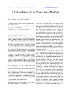
This update rule can be understood as the following. With probability F(y, yp , z, zp )/(π(y)π(yp )), state y bep comes state z while  Z the auxiliary state y remains the same. Alternatively, with probability 1 F(y, yp , x, −zp )dx , no new state (x, yp ) is accepted conditioning on currently being at 1− π(y)π(yp ) Rd state (y, yp ). Instead, state (y, yp ) is directly changed to state (y, −yp ), leading to a different jump process in y. An illustration of the update rule is shown in Fig. 1.

Figure 1: Update rule starting from state (y, yp ). Left: Several possible states (z∗ , zp ) that the algorithm could visit in the next step. Without resampling the auxiliary variables, zp can only be yp or −yp . Right: Assuming the algorithm visits (z1 , yp ) as the next state to (y, yp ) (indicated by the green arrow), a sample trajectory of states generated. From Eq. (24), we see that this proposed algorithm takes the anti-symmetric kernel A(y, yp , z, zp ) to be  1  π(y)π(yp )p(z, zp |y, yp ; ∆t) − π(z)π(zp )p(y, yp |z, zp ; ∆t) (31) A(y, yp , z, zp ) = 2∆t with p(z, zp |y, yp ; ∆t) as in Eq. (29). To ensure correctness of the sampler, A(y, yp , z, zp ) must satisfy (condition 3): Z A(y, yp , z, zp ) dy dyp = 0. Rd+1

In Appendix C.3, we prove that this is indeed the case for A(y, yp , z, zp ) as in Eq. (31). The intuition is that the jump in the auxiliary variable introduces a circulative behavior to the whole process (see Fig. 1 for illustration). This circulation of probability flux is exactly balanced with the jumps in the original variable and the auxiliary variable. We also see in Fig. 1 that irreversibility introduces a directional effect (just like HMC introduces a direction of rotation). This algorithm works well in one dimension, as we demonstrate in Section 6.1. In what follows, we generalize this idea to higher dimensions d > 1. 13

Moving to higher dimensions An irreversible sampler in Rd can be constructed as follows. We expand the state space by introducing a dp -dimensional auxiliary variable yp ∈ Rp in the new state space (y, yp ). The total probability can be designated as: π(y, yp ) = π(y)π(yp ). We further impose symmetry on the auxiliary variables such that π(yp ) = π(−yp ), and let p

fe(z, zp |y, yp ) = p

p

g (z, z |y, y ) = e

d Y

i=1 p

d Y

i=1


H(yip )fi (z|y, yip ) + H(−yip )gi (z|y, −yip ) ;


H(−yip )fi (z|y, −yip ) + H(yip )gi (z|y, yip ) ,

(32)

where fi (z|y, yip ) and gi (z|y, yip ) are conditional probability distributions defined by the value of yip . Calculation of fe and e g is also demonstrated in Algorithm 7 in Appendix C.2. This definition of fe and ge is a direct generalization of the definition of Eq. (27) in the one dimensional case. Fitting this definition into the transition probability p(z, zp |y, yp ; ∆t) in Eq. (29), the generalized update rule is defined and described in Algorithm 4. Again, weRhave the anti-symmetric kernel A(y, yp , z, zp ) as in Eq. (31). As we prove in Appendix C.3, this construction has Rd+dp A(y, yp , z, zp ) dy dyp = 0 even with our dp -dimensional continuous auxiliary variables. In summary, we can use Eq. (29) to devise a practical algorithm for sampling (Algorithm 4). In particular, if we define fi (z|y, yip ) and gi (z|y, yip ) that are easy to sample from, then we can use the definitions of fe and e g in Eq. (32) or Algorithm 7, to propose samples in a similar way as the MH algorithm. After multiple rejections in y, we resample yp according to π(yp ) for a better Markov chain in y. In the experiments of Section 6, we take p p fi (z(∗)|z(t), zp (t)) as (zi (∗) − zi (t))/zpi (t) ∼ Γ(α, β); gi (z(∗)|z(t),  z (t)) as (z(t)  − z(∗))/zi (t) ∼ Γ(α, β) 1 and let π(zp ) to be a restricted uniform distribution on the set zp |zp |1 = 1 . Here fe and ge are designed N to have no overlap in their support, maximizing the irreversibility effect. The norm of zp is set to be constant to ensure that zp contributes to the exploration of direction, instead of the expected distance of jump. In multiple dimensions, a favorable dimension of exploration is often not clear. Hence we suggest to take dp = d, so that zp has the same dimension as z. Thus all directions can be explored by resampling the auxiliary variable zp after multiple rejections. Also, when dp = d, fi and gi can be designed as: fi (z|y) = fi (zi |yi ), and gi (z|y) = gi (zi |yi ), depending only on zi and yi . Sample values in each dimension can thus be independently generated according to fi (zi |yi ) or gi (zi |yi ). When a favorable direction of exploration can be determined (e.g., in the irreversible MALA algorithm in Section 5.2), we can take dp = 1. Then zp belongs to a binary set {−1, 1}, rendering Algorithm 4 the same as the simpler version, Algorithm 3, which is the continuous state space generalization of the “lifting” method [34, 35].

5 Acceptance-Rejection Algorithms with General SDE proposals As discussed in Section 1, there are various ways to combine the continuous dynamics with jump processes to propose new samplers. Since the Markov processes constructed in Section 3 and 4 can all be non-autonomous (resulting in time dependent matrices D, Q and kernel functions S, A) as long as the stationary processes converge to the target distribution, one can iteratively follow continuous dynamics and jump processes to propose samples. With ergodicity, averages with respect to the sample values converge to average with respect to the distribution. This is what is done in HMC: The complete dynamics include a continuous Hamiltonian system with Q equal to the symplectic matrix, and a jump process in the auxiliary variable r with the symmetric kernel S(ry , rz ) = π(ry )π(rz )/∆t, corresponding to the resampling of r. Alternating between the two processes provides the HMC method with exploration across the target distribution and ergodicity. (Note that an important consequence of 14

Algorithm 4: Monte Carlo Algorithm from Irreversible Jump Process for t = 0, 1, 2 · · · do optionally, periodically resample auxiliary variable zp as zp (t) ∼ π(zp ) sample u ∼ U[0,1] sample z(∗) ∼ fe(z(∗), zp (∗)|z(t),(zp (t)) ) π (z(∗)) π (zp (∗)) ge (z(t), zp (t)|z(∗), zp (∗)) p p α (z(t), z (t), z(∗), z (∗)) = min 1, π (z(t)) π (zp (t)) fe(z(∗), zp (∗)|z(t), zp (t)) if u < α (z(t), zp (t), z(∗), zp (∗)), (z(t + 1), zp (t + 1)) = (z(∗), zp (t)) else (z(t + 1), zp (t + 1)) = (z(t), −zp (t)) end

the momentum inversion and resampling, however, is that the resulting HMC dynamics are reversible.) Another straightforward way of combining our continuous and jump processes is to use the continuous dynamic sampler for some variables (e.g., real-valued variables) and the jump process sampler for others (e.g., discrete-valued variables). In addition to the aforementioned means of combining continuous dynamics with jump processes for sampling, in this section we discuss how to use the continuous dynamics as a proposal distribution in our jump process acceptreject scheme, even when the continuous dynamics are not reversible. This approach relies on the irreversible jump sampler of Algorithm 4 using general continuous Markov processes (SDEs) as proposals. Previously, similar methods such as the Metropolis Adjusted Langevin diffusion (MALA) and Riemannian Metropolis Adjusted Langevin diffusion (RMALA) [31, 38, 18] have only been proposed for reversible processes. They use one step integration of reversible SDEs to propose samples and use the MH algorithm to accept or reject the proposal. In this section, we extend these methods to include proposals from any SDE in the form of Eq. (13) (any SDE with a mild integrability condition), without the requirement of reversibility. In Section 6, we show that this combination can generate better results for correlated distributions.

5.1 General SDE Proposals under Small Step Size Limit Our ultimate goal is to use the stochastic dynamics of Eq. (13) to propose samples in the framework of Algorithm 3. In practice, we need to simulate from the discretized SDE of Eq. (16). Before analyzing this case, we first examine what would happen if we could exactly simulate the SDE of Eq. (13).
Here, we take f (z|y, yp ) in Eq. (32) to be a Markov transition kernel P z|y; dt defined via an infinitesimal step dt in the SDE: h i p
(33) dz = − D(z) + Q(z) ∇H(z) + Γ(z) dt + 2D(z)dW(t), P

∂ (Dij (z) + Qij (z)). ∂zj
For the reverse proposal g(z|y, yp ) in Eq. (32), we use the adjoint process P † z|y; dt , inverting the irreversible dynamics via Q(z) → −Q(z) [25]: h i p
e dz = − D(z) − Q(z) ∇H(z) + Γ(z) dt + 2D(z)dW(t), (34)

where Γi (z) =

e i (z) = where Γ

j

P

j

∂ (Dij (z) − Qij (z)). ∂zj

15



Theorem 2. For the Markov processes P z(T ) |z(t) ; (T − t) and P † z(T ) |z(t) ; (T − t) defined by the SDEs of Eq. (33) and Eq. (34) through Itˆo integral, the following equality holds:

P z(T ) |z(t) ; (T − t) π z(T )
=
. (35) P † z(t) |z(T ) ; (T − t) π z(t) The proof is in Appendix D. Using Theorem 2, we have (
)   π (z∗ ) P † z(t) |z∗ ; (T − t) (t) ∗

= 1. α z , z = min 1, π z(t) P z∗ |z(t) ; (T − t)

(36)

Even though in Section 3, we saw that SDEs of the form in Eq. (13) have π(z) as the invariant distribution, it is not immediately obvious that using this SDE as a proposal in Algorithm 3 would lead to an acceptance rate of 1. This is a nice result, however, because it gives us insight into the fact that using more accurate numerical integrators could lead to higher acceptance rates. In Section 5.2, we analyze the accept-reject scheme for the simple first-order integration of Eq. 16 with finite step size ∆t.

5.2 Generalizing the Metropolis-Adjusted Langevin Algorithm to Irreversible MALA Since in practice we rely on finite step sizes ∆t > 0, there will be numerical error and


P z∗ |z(t) ; ∆t
can differ P † z(t) |z∗ ; ∆t

π (z∗ )
. We now propose a generalization of the MALA algorithm to correct for these errors. We make use π z(t) of Algorithm 3 and take a general SDE and its adjoint process defined in Section 5.1 to propose samples using a one-step numerical integration (as in MALA). Because we have the local gradient information in the SDEs to guide us, the direction of the exploration is determined. So, we simply use a 1-dimensional discrete auxiliary variable yp , and thus the use of Algorithm 3 instead of the more general Algorithm 4. We call the resulting algorithm the irreversible MALA method. Assuming a one-step numerical integration uses a ∆t period of time, then the discretization of the SDE of Eq. (33) leads to   1 P (z|y; ∆t) ∝ exp − G(y, z)T D(y)−1 G(y, z) , (37) 4∆t

from

where

h i
G(y, z) = (z − y) − − D(y) + Q(y) ∇H(y) + Γ(y) ∆t.

Importantly, this allows us to compute f (z(∗)|z(t)) = P (z(∗)|z(t); ∆t) in Algorithm 3. The corresponding calculation for the adjoint process with the SDE in Eq. (34) is:   1 G† (y, z)T D(y)−1 G† (y, z) , (38) P † (z|y; ∆t) ∝ exp − 4∆t where

h i
G† (y, z) = (z − y) − − D(y) − Q(y) ∇H(y) + Γ(y) ∆t.

This allows us to compute g (z(∗)|z(t)) = P † (z(∗)|z(t); ∆t). The resulting irreversible MALA algorithm is summarized in Algorithm 5.

16

Algorithm 5: Irreversible MALA randomly pick z p from {1, −1} with equal probability for t = 0, 1, 2 · · · do optionally, periodically resample auxiliary variable z p ∼ U{1,−1} sample u ∼ U[0,1] if z p > 0 then 
 z(∗) ← zt − ǫt D(zt ) + Q(zt ) ∇H(zt ) + Γ(zt ) + N (2ǫt D(zt ))   π (z(∗)) P † (z(t)|z(∗); ∆t) α (z(t), z(∗)) = min 1, π (z(t)) P (z(∗)|z(t); ∆t) end else 
 + N (2ǫt D(zt )) z(∗) ← zt − ǫt D(zt ) − Q(zt ) ∇H(zt ) + Γ(zt )  π (z(∗)) P (z(t)|z(∗); ∆t) α (z(t), z(∗)) = min 1, π (z(t)) P † (z(∗)|z(t); ∆t) end if u < α (z(t), z(∗)), z(t + 1) = z(∗); z p (t + 1) = z p (t) else z(t + 1) = z(t); z p (t + 1) = −z p (t) end
We know from Section 5.1 that in the small ∆t limit, α z(t) , z∗ = 1. Indeed,

P (z|y; ∆t) π(y) · P † (y|z; ∆t) π(z)  
π(y) 1 † T −1 † T −1 G (z, y) D(z) G (z, y) − G(y, z) D(y) G(y, z) = exp 4∆t π(z)

→1.

(39)

From this, we see that there seems to be a step-size/acceptance-rate tradeoff. As mentioned in Section 5.1, a higher-order numerical scheme could potentially increase the acceptance rate with the same step size, and is left as a direction for future research.

6 Experiments To examine the correctness and attributes of our irreversible jump sampler (Algorithm 4), we consider various simulated scenarios, including the challenging cases of heavy tail, multimodal, and correlated distributions. As (z(∗)|z(t), zp (t))  as mentioned in Section 4.3, we take fi (z(∗)|z(t), zp (t)) as (zi (∗) − zi (t))/zpi (t) ∼ Γ(α, β); gi  1 p p p p (z(t) − z(∗))/zi (t) ∼ Γ(α, β) and let π(z ) to be a restricted uniform distribution on the set z |z |1 = 1 . N In Appendix E, we specify the settings of α and β. These hyperparameters were chosen using a generic procedure without fine-tuning to the target.

6.1 1D Heavy-tailed Distribution We start by considering the task of sampling from 1D normal and log-normal distributions, the latter of which is a heavy-tailed distribution. The motivation for considering the simple 1D normal distribution is to validate

17

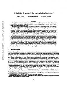
the correctness of the sampler and to serve as a comparison relative to the heavy tailed setting. We compare performance to a MH algorithm with normal proposals centered at the previous state. The results are shown in Fig. 2. Some may argue that the main possible benefit of our sampler arises from the gamma proposal distribution. To test this idea, we also compare against an MH algorithm using a symmetrized gamma proposal distribution: 1 (z(∗) − z(t)) ∼ (f (z(∗)|z(t)) + g (z(∗)|z(t))). 2

0.0001

1

Log Normal Gaussian

5

-5

5

10

0 1

−2

0.8

ACF

log(T−V Distance)

1.2

−1

−3 −4

Gauss RW MH Gamma Irreversible Gamma RW MH

−5 −8

−6

−4

−2

Gauss RW MH Gamma Irreversible Gamma RW MH

0.6 0.4 0.2 0

0

2

log (run−time)

−0.2 0

3

0.5

1

run−time lag 1.2

Gauss RW MH Gamma Irreversible Gamma RW MH

1

−1

0.8

−2

ACF

log(T−V Distance)

0

−3 −4 −5 −8

1.5 −5

x 10

Gauss RW MH Gamma Irreversible Gamma RW MH −6

−4

−2

0.6 0.4 0.2 0

0

−0.2 0

2

log (run−time)

0.5

run−time lag

3

1

1.5 −5

x 10

Figure 2: Top row: (Left) normal and log-normal target distributions, and (right) zoom in of the tail distributions. Middle row: Results for normal target in terms of log total variation distance (T-V distance) vs. log run time (left) and ACF vs. lag in run time (right). Bottom row: Analogous plots for log normal target. Comparisons are made among the irreversible jump sampler of Algorithm 4 (Gamma Irreversible), random walk MH algorithm with Gaussian proposals (Gauss RW MH), and random walk MH algorithm with symmetrized Gamma proposals (Gamma RW MH). Rum time is measured in seconds. We found that the irreversible jump sampler with the gamma proposals has better performance. The reason is that it can decrease autocorrelation without increasing the rejection rate (the rejection rate of all three methods are similar). The MH algorithm with symmetrized gamma proposals, on the other hand, leads to even higher 18

autocorrelation than the vanilla MH algorithm. Intuitively, this result can be understood from Fig. 1: the irreversible algorithm leads to further exploration in one direction before circling back. In the heavy-tailed distribution, similar behavior is observed: the irreversible jump sampler converge to the desired distribution faster because its samples decorrelate more rapidly over run time.

6.2 Multimodal Distributions 6.2.1 2D Bimodal distributions We use our irreversible jump sampler to sample increasingly challenging bimodal distributions in 2D, π(z1 , z2 ) = 2 ∗ (z12 − τ )2 − 0.2z1 − 5z12 + 5z22 , displayed in Fig. 3. Based on the results of Section 6.1, we simply compare against MH with random walk normal proposals and drop the symmetrized gamma proposal case. In Fig. 3 we see that the irreversible jump sampler significantly outperforms the random walk MH algorithm. Intuitively, this is facilitated by the greater traversing ability of the irreversible sampler, so that with the same acceptance rate, the irreversible sampler can explore more possible states than the reversible ones, and have greater chance of transiting into another mode. One way to capture this difference in the bimodal case is in terms of escape time from local modes, which we summarize in Table 1. We see that the irreversible jump sampler has escape times orders of magnitude lower and increase at a much smaller rate, indicating much more rapid mixing between modes.

19

Τ=0.5 Τ=1 Τ=1.5

2

2

1

1

0

0

−1

−1

−2

−2

0

1

2 3 time (s)

1

0

1

2 3 time (s)

4

5

Gauss RW MH Gamma Irreversible

0.8

0.6

ACF

T−V Distance

5

1

Gauss RW MH Gamma Irreversible

0.8

0.4

0.6 0.4

0.2 0 −8

4

0.2

−6

−4

−2

0

2

0 0

4

log3(run−time)

0.5

1

1.5

2

2.5

run−time lag

3 −5

x 10

τ = 0.5 1

1.2

Gauss RW MH Gamma Irreversible

1 0.8

0.6

0.6

ACF

T−V Distance

0.8

0.4

Gauss RW MH Gamma Irreversible

0.4 0.2

0.2 0 0 −8

−6

−4

−2

0

2

−0.2 0

4

log (run−time)

0.2

0.4

0.6

0.8

run−time lag

3

1 −4

x 10

τ =1 1

1

Gauss RW MH Gamma Irreversible

0.8

0.6

ACF

T−V Distance

0.8

0.4

0.6 0.4

0.2 0 −8

Gauss RW MH Gamma Irreversible

0.2

−6

−4

−2

0

2

0 0

4

log3(run−time)

0.2

0.4

0.6

run−time lag

0.8

1 −4

x 10

τ = 1.5 Figure 3: Top row: (Left) Bimodal targets, π(z1 , z2 ) = 2(z12 − τ )2 − 0.2z1 − 5z12 + 5z22 , for various values of τ . Here we demonstrate a 1D cross section of the 2D distribution. (Middle) Sample state trajectories for MH and (right) irreversible jump sampler for the τ = 1 case. Bottom rows: Total variational distance vs. log run time (left) and ACF vs. lag in run time (right), with each row corrresponding to a specific choice of τ . 20

τ 0.5 1 1.5 2

Avg. Escape Time for Irr. Sampler 1.94 × 102 4.64 × 102 9.06 × 102 2.41 × 103

Avg. Escape Time for MH Sampler 1.06 × 103 2.47 × 104 7.89 × 105 N/A

Table 1: Comparison of average escape time from one local mode to another between the irreversible jump sampler and random walk MH. The distribution in 2D is more challenging with bigger values of τ (plotted in Fig. 3). “N/A” in the last entry means that the escape time is so long that an accurate estimate of it is not available. 6.2.2 2D Multimodal distributions We also tested our method against a recently considered multimodal setting [32]. In the first setting considered, the target distribution is highly multimodal with 2D unevenly distributed modes. Furthermore, the high mass modes have smaller radii of variation. In the second setting considered, these modes are highly concentrated and well separated, which is extremely challenging for most samplers. See Figs. 4 and 5. In [32], a repulsive attractive Metropolis (RAM) sampler was proposed with a structure specifically designed to efficiently handle these types of multimodal distributions. We use this as a gold-standard comparison, since this method was already shown to outperform parallel tempering and alternatives [22] in this setting. In these settings, we focus our performance analysis on the decay speed of the autocorrelation function (ACF). This can be understood by taking the Gaussian random walk MH algorithm as an example: Although the Gaussian random walk MH algorithm seems to perform well in terms of convergence of total variation distance, this effect is based on exploring one mode really well in a short period of time, instead of making more distant moves to explore other modes. In contrast, the ACF better characterizes the exploration of the samples through the whole space. Our results are summarized in Figs. 4 and 5 for each of the two simulated multimodal scenarios. In the first scenario, our sampler outperforms both MH and RAM. In the second scenario, where we have highly concentrated and separated modes, the RAM method tailored to this scenario slightly outperforms our approach. Overall, however, the irreversible jump sampler provides surprisingly good performance in these scenarios despite not having been designed specifically for this setting.

6.3 Correlated Distribution We also test our algorithm on a highly correlated (moon-shaped) target distribution, where π(z1 , z2 ) = z14 /10 + (4(z2 + 1.2) − z12 )2 /2. In terms of number of iterations, the irreversible jump sampler with Gamma proposals decorrelates and converges to the posterior distribution faster (c.f. Fig. 9 in Appendix E.1). However, in terms of run time, our sampler does not perform as well as random walk MH algorithm, as explored in Fig. 6. The reason is that the correlated distribution has complex geometry. Faster exploration in random directions, as provided by our irreversible sampler with independent proposals, only marginally increases the mixing effect in each step relative to the reversible independent proposals of MH. Since the calculation of the distribution is not demanding in this case, the small overhead of the irreversible sampler (keeping track of the number of rejections and resample the direction of exploration after multiple rejections) actually makes a difference and thus results in our sampler with gamma proposals providing slightly worse performance in terms of runtime. Note that in terms of per iteration performance, our sampler’s performance exceeds that of MH. To improve the performance of our irreversible sampler further in this correlated target case, it would be appealing to take the geometric information about the level sets—including the higher mass regions—into account. Indeed, we are able to do this by replacing the independent gamma proposals with proposals from our continuous dynamics sampler, as described in Section 5. To demonstrate the effect of irreversibility, we choose

21

10

T−V Distance

8 6 4 2

1

1

0.8

0.8

0.6

0.6

ACF

12

0.4

0.4

Gauss RW MH Gamma Irreversible RAM

0.2

0 −2 −2

0

2

4

6

8

10

0 −4

12

−2

0

0.2

2

4

0 0

6

log3(run−time) 12

12

10

10

10

8

8

8

6

6

6

4

4

4

2

2

2

0

0 0

2

4

6

8

10

12

1

2

3

4

run−time lag

12

−2 −2

Gauss RW MH Gamma Irreversible RAM

5 −5

x 10

0

−2 −2

0

2

4

6

8

10

−2 −2

12

0

2

4

6

8

10

12

Figure 4: Top row: (Left) Contour plot of a challenging multimodal probability density function; (middle) T-V distance and ACF comparisons among Gauss RW MH algorithm, Gamma Irreversible, and the recently proposed repulsive attractive Metropolis (RAM) sampler. Bottom row: A sample run of all three samplers, respectively.

10

T−V Distance

8 6 4 2

1

1

0.8

0.8

0.6

0.6

ACF

12

0.4

0.4

Gauss RW MH Gamma Irreversible RAM

0.2

0 −2 −2

0

2

4

6

8

10

0 −6

12

Gauss RW MH Gamma Irreversible RAM

−4

−2

0

0.2

2

4

6

log (run−time)

0 0

0.5

12

12

12

10

10

10

8

8

8

6

6

6

4

4

4

2

2

2

0

0

0

−2 −2

−2 −2

−2 −2

0

2

4

6

8

10

12

0

2

4

6

8

1

1.5

run−time lag

3

10

12

0

2

4

6

−4

x 10

8

10

12

Figure 5: Plots as in Fig. 4, but for an even more challenging multimodal case where the modes are very concentrated and well separated. 

   2 0 0 −2 and Q(z) = in Eqs. (33), (34), (37), and (38). In this case, our irreversible 0 2 2 0 MALA algorithm (Algorithm 5) significantly outperforms the Gaussian random walk MH, as well as HMC [28] and the standard reversible MALA algorithm [31]. Because the target distribution has complex geometry, the continuous dynamics can provide guidance on locating the higher mass regions and exploring the contours rapidly with the gradient information. HMC and MALA algorithms exploit this effect, but we additionally see gains from D(z) =

22

1

3 2

Gauss RW MH Gamma Irreversible

0.8

ACF

1 0

0.6 0.4

−1

0.2

−2 −3 −3

−2

−1

0

1

2

0 0

3

Gauss RW MH Gamma Irreversible

Gauss RW MH Irreversible MALA HMC MALA

0.8 T−V Distance

0.8

T−V Distance

2 −4

x 10

1

1

0.6 0.4

0.6 0.4 0.2

0.2 0 −8

1

run−time lag

−6

−4

−2

0

2

0 −8

4

log3(run−time)

−6

−4 −2 log (run−time)

0

2

3

Figure 6: Top row: Correlated distribution with complex geometry in 2D, π(z1 , z2 ) = z14 /10+(4(z2+1.2)−z12)2 /2 (left) and ACF vs. lag in run time of Gamma Irreversible algorithm against Gauss RW MH (right). Bottom row: T-V distance vs. log run time. Comparisons are made between Gauss RW MH and Gamma Irreversible (left), and Gauss RW MH, Irreversible MALA, HMC, and MALA (right). irreversible sampler. This experiment demonstrates the gains that are possible by combining our continuous dynamics and jump process frameworks, beyond what either can provide individually.

7 Scaling Up the Sampling Algorithms for Large Data Sets We wish to scale up the previously discussed sampling algorithms to cases where our target distribution is a posterior distribution in a Bayesian model, and we are faced with a huge number of observations. In this case, the likelihood, or its gradient, can be computationally prohibitive to compute. For the samplers designed from continuous dynamics (Section 3), we use stochastic gradients in place of the full data gradient. For samplers using jump processes (Section 4), we discuss a generalization of the subsamplingwithin-MH ideas in [21, 2, 3].

7.1 Stochastic Gradient Samplers For samplers using continuous dynamics (Eq. (13)), we can see that the computationally intensive component in the update rule of Eq. (16) is the computation of ∇H(zt ), which can be explained as follows. Assume that the data s ∈ S are i.i.d.: s ∼ p(s|θ). We P write our posterior distribution as p(θ|S) ∝ exp(−U (θ)), where the potential function U is given by U (θ) = − s∈S log p(s|θ) − log p(θ). Recall that we have set our total target distribution 23

as: π(z) = p(S|θ) p(r). Hence, H(z) =PU (θ) + ln p(r). Calculating the gradient of H(z) involves evaluating the gradient of U (θ). That is: ∇U (θ) = − s∈S ∇ log p(s|θ) − ∇ log p(θ). When the amount of data is large, U (θ) can be too computationally intensive to calculate as it relies on a sum over all data points. One idea for avoiding this per iteration cost is to use stochastic gradients instead. Here, a noisy gradient based on a data subsample or minibatch, is used as an unbiased estimator of the full data gradient of Eq. (13). More formally, we examine independently sampled minibatches Se ⊂ S. The corresponding potential for these data is e (θ) = − |S| U e |S|

X

log p(s|θ) − log p(θ);

s∈Se

Se ⊂ S.

(40)

e (θ) is an unbiased estimator of U (θ). As such, a gradient computed The specific form of Eq. (40) implies that U e based on U (θ)—called a stochastic gradient [30]—is a noisy, but unbiased estimator of the full-data gradient. The key question in many of the existing stochastic gradient MCMC algorithms is whether the noise injected by the e (θ) in place of stochastic gradient adversely affects the stationary distribution of the modified dynamics (using ∇U ∇U (θ)). One way to analyze the impact of the stochastic gradient is to make use of the central limit theorem and assume e (θ) = ∇U (θ) + N (0, V(θ)), ∇U (41) e e resulting in a noisy Hamiltonian gradient ∇H(z) = ∇H(z) + [N (0, V(θ)), 0]T . Simply plugging in ∇H(z) in
place of ∇H(z) in Eq. (16) results in dynamics with an additional noise term (D(zt ) + Q(zt ) [N (0, V(θ)), 0]T . ˆ t of the variance of this additional noise satisfying 2D(zt ) − To counteract this, assume we have an estimate B ˆ ǫt Bt  0 (i.e., positive semidefinite). With small ǫ, this is always true since the stochastic gradient noise scales down faster than the added noise. Then, we can attempt to account for the stochastic gradient noise by simulating h i
ˆ t )). e t ) + Γ(zt ) + N (0, ǫt (2D(zt ) − ǫt B (42) zt+1 ← zt − ǫt D(zt ) + Q(zt ) ∇H(z

Comparing to the original update rule in Eq. (13), the full data gradient is replaced by the stochastic gradient, and ˆ t . This provides our stochastic gradient—or minibatch— the variance of the injected noise is subtracted by ǫt B variant of the sampler. In Eq. (42), the noise introduced by the stochastic gradient is multiplied by ǫt (and the compensation by ǫ2t ), implying that the discrepancy between these dynamics and those of Eq. (16) approaches zero as ǫt goes to zero. As such, in this infinitesimal step size limit, since Eq. (16) yields the correct invariant distribution, so does Eq. (42). This avoids the need for a costly or potentially intractable MH correction. However, having to decrease ǫt to zero comes at the cost of increasingly small updates. We can also use a finite, small step size in practice, resulting in a biased (but faster) sampler. A similar bias-speed tradeoff was used in [21, 2, 3] to construct MH samplers (see Section 7.2), in addition to being used in SGLD and SGHMC. For the irreversible (and reversible) MALA algorithms, if an accurate estimate of the stochastic gradient noise is available, the stochastic gradient method can combine with the subsampling approach in Section 7.2 to provide scalable variants of the MALA algorithms. 7.1.1 Previous Stochastic Gradient MCMC Algorithms as Special Examples We explicitly state how some recently developed MCMC methods fall within the proposed framework based on specific choices of D(z), Q(z) and H(z). Stochastic Gradient Hamiltonian Monte Carlo (SGHMC) As discussed in [10], simply replacing ∇U (θ) by e (θ) in Eq. (17) results in the following updates: the stochastic gradient ∇U  θt+1 ← θt + ǫt M−1 rt (43) Naive : e (θt ) ≈ rt − ǫt ∇U (θt ) + N (0, ǫ2 V(θt )), rt+1 ← rt − ǫt ∇U t 24

where the ≈ arises from the approximation of Eq. (41). Careful study shows that Eq. (43) cannot be rewritten into our proposed framework, which hints that such a na¨ıve stochastic gradient version of HMC is not correct. Interestingly, the authors of [10] proved that this na¨ıve version indeed does not have the correct stationary distribution. In our framework, we see that the noise term N (0, 2ǫtD(z)) is paired  with a D(z)∇H(z) term, hinting that such a 0 0 , which means we need to add D(z)∇H(z) term should be added to Eq. (43). Here, D(θ, r) = 0 ǫV(θ) = ǫV(θ)∇r H(θ, r) = ǫV(θ)M−1 r. This is the correction strategy proposed in [10], but through a physical interpretation of the dynamics. In particular, the term ǫV(θ)M−1 r (or, generically, CM−1 r where C  ǫV(θ)) has an interpretation as friction and leads to second order Langevin dynamics:  θt+1 ← θt + ǫt M−1 rt (44) ˆ t )). e (θt ) − ǫt CM−1 rt + N (0, ǫt (2C − ǫt B rt+1 ← rt − ǫt ∇U

ˆ t is an estimate of V(θt ). This method now fits into our framework with H(θ, r) and Q(θ, r) as in HMC, Here, B   0 0 but with D(θ, r) = . This example shows how our theory can be used to identify invalid samplers 0 C and provide guidance on how to effortlessly correct the mistakes; this is crucial when physical intuition is not available. Once the proposed sampler is cast in our framework with a specific D(z) and Q(z), there is no need for sampler-specific proofs, such as those of [10]. Stochastic Gradient Langevin Dynamics (SGLD) momentum) Langevin dynamics to generate samples

SGLD [36] proposes to use the following first order (no

e (θt ) + N (0, 2ǫt D). θt+1 ← θt − ǫt D∇U

(45)

ˆ t = 0. As motivated This algorithm corresponds to taking z = θ with H(θ) = U (θ), D(θ) = D, Q(θ) = 0, and B by Eq. (42) of our framework, the variance of the stochastic gradient can be subtracted from the sampler injected noise to make the finite stepsize simulation more accurate. This variant of SGLD leads to the stochastic gradient Fisher scoring algorithm [1]. Stochastic Gradient Riemannian Langevin Dynamics (SGRLD) SGLD can be generalized to use an adaptive diffusion matrix D(θ). Specifically, it is interesting to take D(θ) = G−1 (θ), where G(θ) is the Fisher information metric. The sampler dynamics are given by e (θt ) + Γ(θt )] + N (0, 2ǫt G(θt )−1 ). θt+1 ← θt − ǫt [G(θt )−1 ∇U

(46)

ˆ t = 0, this SGRLD [29] method falls into our framework with Taking D(θ) = G(θ)−1 , Q(θ) = 0, and B P ∂Dij (θ) correction term Γi (θ) = . It is interesting to note that in earlier literature [18], Γi (θ) was taken to ∂θj j
P ∂ 1/2 be 2 |G(θ)|−1/2 G−1 . More recently, it was found that this correction term corresponds ij (θ)|G(θ)| j ∂θj to the distribution function with respect to a non-Lebesgue measure [31]; for the Lebesgue measure, the revised Γi (θ) was as determined by our framework [31]. Again, we have an example of our theory providing guidance in devising correct samplers. Stochastic Gradient Nos´e-Hoover Thermostat (SGNHT) Finally, the SGNHT [14, 37] method incorporates ideas from thermodynamics to further increase adaptivity by augmenting the SGHMC system with an additional

25

scalar auxiliary variable, ξ. The algorithm uses the following dynamics:  θt+1 ← θt + ǫt rt    ˆ e rt+1 ← rt − ǫt ∇ U (θt ) − ǫt ξt rt + N (0, ǫt (2A − ǫt Bt )) 1 T    ξt+1 ← ξt + ǫt r rt − 1 . d t  0 0 1 1 We can take z = (θ, r, ξ), H(θ, r, ξ) = U (θ)+ rT r+ (ξ −A)2 , D(θ, r, ξ) = 00 A0· I 2 2d  0  −I 0 I 0 r/d to place these dynamics within our framework. T 0

−r

/d

(47)

0 0 0

 , and Q(θ, r, ξ) =

0

Summary In our framework, SGLD and SGRLD take Q(z) = 0 and instead stress the design of the diffusion matrix D(z), with SGLD using a constant D(z) and SGRLD an adaptive, θ-dependent diffusion matrix to better account for the geometry of the space being explored. On the other hand, HMC takes D(z) = 0 and focuses on the curl matrix Q(z). SGHMC combines SGLD with HMC through non-zero D(θ) and Q(θ) matrices. SGNHT then extends SGHMC by taking Q(z) to be state dependent. We readily see that most of the product space D(z)×Q(z), defining the space of all possible samplers, has yet to be filled. 7.1.2 Stochastic Gradient Riemann Hamiltonian Monte Carlo In Section 7.1.1, we have shown how our framework unifies existing samplers. In this section, we now use our framework to guide the development of a new sampler. While SGHMC [10] inherits the momentum term of HMC, making it easier to traverse the space of parameters, the underlying geometry of the target distribution is still not utilized. Such information can usually be represented by the Fisher information metric [18], denoted as G(θ), which can be used to precondition the dynamics. For our proposed system, we consider H(θ, r) = U (θ) + 21 rT r, as in HMC/SGHMC methods, and modify the D(θ, r) and Q(θ, r) of SGHMC to account for the geometry as follows:     0 −G(θ)−1/2 0 0 ; Q(θ, r) = . D(θ, r) = −1 −1/2 0

G(θ)

G(θ)

0

We refer to this algorithm as stochastic gradient Riemann Hamiltonian Monte Carlo (SGRHMC). Our theory holds for any positive definite G(θ), yielding a generalized SGRHMC (gSGRHMC) algorithm, which can be helpful when the Fisher information metric is hard to compute. A na¨ıve implementation of a state-dependent SGHMC algorithm might simply (i) precondition the HMC upe (θ), and (iii) add a state-dependent friction term on the order of the diffusion matrix date, (ii) replace ∇U (θ) by ∇U to counterbalance the noise as in SGHMC, resulting in:  θt+1 ← θt + ǫt G(θt )−1/2 rt Naive : (48) −1/2 −1 −1 e ˆ rt+1 ←

rt − ǫt G(θt )

∇θ U (θt ) − ǫt G(θt )

rt + N (0, ǫt (2G(θt )

− ǫt Bt )).

However, as we show in Section 7.3.1, samples from these dynamics do not converge to the desired distribution. Indeed, this system cannot be written within our framework. Instead, we can simply follow our framework and, as indicated by Eq. (42), consider the following update rule: ( θt+1 ← θt + ǫt G(θt )−1/2 rt

  ˆ t )), e (θt ) + ∇θ G(θt )−1/2 − G(θt )−1 rt ] + N (0, ǫt (2G(θt )−1 − ǫt B rt+1 ← rt − ǫt [G(θ)−1/2 ∇θ U

(49)



P ∂ G(θ)−1/2 ij . The practical imwhich includes a correction term ∇θ G(θ)−1/2 , with i-th component ∂θ j j plementation of gSGRHMC is outlined in Algorithm 6. 26

Algorithm 6: Generalized Stochastic Gradient Riemann Hamiltonian Monte Carlo initialize (θ0 , r0 ) for t = 0, 1, 2 · · · do optionally, periodically resample momentum r as r(t) ∼ N (0, I) ˆ t) θt+1 ← θt + ǫt G(θt )−1/2 rt , Σt ← ǫt (2G(θt )−1 − ǫt B   −1/2 −1/2 e (θt ) + ǫt ∇θ (G(θt ) ) − ǫt G(θt )−1 rt + N 0, Σt rt+1 ← rt − ǫt G(θt ) ∇θ U end

7.2 Subsampling of Irreversible Sampler from Jump Processes For the irreversible jump sampler (Algorithm 4), we can directly generalize the subsampling idea for the MH algorithms [21] and its adaptive and proxy method variations [2, 3]. In Algorithm 4, the computational bottleneck is at the step where we decide to accept or reject the proposal from sampling fe(θ(∗), θp (∗)|θ(t), θp (t)), since we need to calculate π(θ(∗))/π(θ(t)), requiring information from the entire likelihood. This accept-reject step is implemented by sampling the uniform random variable u ∼ U[0,1] and accepting the proposal if and only if u
ΘS (u, θ(t), θ(∗), θp (t), θp (∗)),

(51)

  1 X p(s|θ(∗)) ΛS (θ(t), θ(∗)) = , log |S| p(s|θ(t))

(52)

where

s∈S

and # " 1 π (θp (t)) fe(θ(∗), θp (∗)|θ(t), θp (t)) ΘS (u, θ(t), θ(∗), θ (t), θ (∗)) = . log u |S| π (θp (∗)) ge (θ(t), θp (t)|θ(∗), θp (∗)) p

p

For the computationally intractable ΛS (θ(t), θ(∗)), we can use a subset of data to approximate it with:   1 X p(s|θ(∗)) ∗ ΛSe(θ(t), θ(∗)) = ≈ ΛS (θ(t), θ(∗)); Se ⊂ S. log e p(s|θ(t)) |S|

(53)

(54)

s∈Se

Importantly, |ΛS (θ(t), θ(∗)) − Λ∗Se(θ(t), θ(∗))| can be bounded probabilistically [2]. Hence, a speed-bias tradeoff can be quantified through the probabilistic bounds when we use Λ∗Se(θ(t), θ(∗)) instead of ΛS (θ(t), θ(∗)). In some cases more data can be used to tighten or approximate the bound on |ΛS (θ(t), θ(∗)) − Λ∗Se(θ(t), θ(∗))|, so that inequality (50) can always be verified. Then the above procedure still yields an exact sampler. In many cases, however, so much data has to be used that the computation gains of subsampling are hard to see. As such, we typically view this scheme as one with quantifiable bias. See [3] for further discussions and developments. Overall, due to the similarities between our irreversible jump sampler and the MH algorithm, many methods developed specifically for MH can be applied in our context, which is quite appealing. For example, as discussed 27

1

Naive gSGRHMC T−V Distance

T-V Distance

0.8

1

0.010 0.008

2

0.006 0.004

SGLD

0.4 0.2

2

0.002 0.000

0.6

SGHMC 1

1

2

gSGRHMC 1

2

0 −6

SGLD SGHMC gSGRHMC −4

−2

0

log3(run−time)

2

Figure 7: Left: For two simulated 1D distributions defined by U (θ) = θ2 /2 (one peak) and U (θ) = θ4 − 2θ2 (two peaks), we compare the KL divergence of methods: SGLD, SGHMC, the na¨ ıve SGRHMC of Eq. (48), and the gSGRHMC of Eq. (49) relative to the true distribution in each scenario (left and right bars labeled by 1 and 2). Right: For a correlated 2D distribution with U (θ1 , θ2 ) = θ14 /10 + (4 · (θ2 + 1.2) − θ12 )2 /2, we see that our gSGRHMC most rapidly explores the space relative to SGHMC and SGLD. Contour plots of the distribution along with paths of the first 10 sampled points are shown for each method. above, we have directly applied the subsampling approach designed for scaling MH to our approach. We can also combine our irreversible jump sampler with the RAM algorithm to further improve exploration power in the case of multimodal targets.

7.3 Experiments In Section 7.3.1, we show that gSGRHMC can excel at rapidly exploring distributions with complex landscapes. We then apply SGRHMC to sampling in a latent Dirichlet allocation (LDA) model on a large Wikipedia dataset in Section 7.3.2. Appendix F contains details on the specific samplers considered and the parameter settings used in these experiments. 7.3.1 Synthetic Experiments In this section we aim to empirically (i) validate the correctness of our recipe and (ii) assess the effectiveness of gSGRHMC. In Fig. 7(left), we consider two univariate distributions (shown in the Supplement) and compare SGLD, SGHMC, the na¨ıve state-adaptive SGHMC of Eq. (48), and our proposed gSGRHMC of Eq. (49). See the Supplement for the form of G(θ). As expected, the na¨ıve implementation does not converge to the target distribution. In contrast, the gSGRHMC algorithm obtained via our recipe indeed has the correct invariant distribution and efficiently explores the distributions. In the second experiment, we sample a bivariate distribution with strong correlation. The results are shown in Fig. 7(right). The comparison between SGLD, SGHMC, and our gSGRHMC method shows that both a state-dependent preconditioner and Hamiltonian dynamics help to make the sampler more efficient than either element on its own. 7.3.2 Online Latent Dirichlet Allocation We also applied SGRHMC (with G(θ) = diag(θ)−1 , the Fisher information metric) to an online latent Dirichlet allocation (LDA) [6] analysis of topics present in Wikipedia entries. In LDA, each topic is associated with a distribution over words, with βkw the probability of word w under topic k. Each document is comprised of a (d) mixture of topics, with πk the probability of topic k in document d. Documents are generated by first selecting

28

Parameter θ Prior p(θ)

Method SGLD SGHMC SGRLD SGRHMC

Original LDA βkw = θkw p(θk ) = Dir(α)

Expanded Mean βkw = Pθkw w θkw p(θkw ) = Γ(α, 1)

Average Runtime per 100 Docs 0.778s 0.815s 0.730s 0.806s

3500

SGLD SGHMC SGRLD SGRHMC

Perplexity

3000 2500 2000 1500 1000 0

2000

4000

6000

Number of Documents

8000

10000

Figure 8: Top: Expanded mean parameterization of the LDA model. Middle: Average runtime per 100 Wikipedia entries for all methods. Bottom: Perplexity versus number of Wikipedia entries processed.

29

(d)

a topic zj π

(d)

∼ π (d) for the jth word and then drawing the specific word from the topic as xj

∼ βz(d) . Typically, j

(d)

and βk are given Dirichlet priors. The goal of our analysis here is inference of the corpus-wide topic distributions βk . Since the Wikipedia dataset is large and continually growing with new articles, it is not practical to carry out this task over the whole dataset. Instead, we scrape the corpus from Wikipedia in a streaming manner and sample parameters based on minibatches of data. Following the approach in [29], we first analytically marginalize the document distributions π (d) and, to resolve the boundary issue posed by the Dirichlet posterior of βk defined on the probability simplex, use an expanded mean parameterization shown in Figure 8(upper left). Under this parameterization, we then compute ∇ log p(θ|x) and, in our implementation, use boundary reflection to ensure the positivity of parameters θkw . The (d) necessary expectation over word-specific topic indicators zj is approximated using Gibbs sampling separately on each document, as in [29]. The Supplement contains further details. For all the methods, we report results of three random runs. When sampling distributions with mass concentrated over small regions, as in this application, it is important to incorporate geometric information via a Riemannian sampler [29]. The results in Fig. 8(right) indeed demonstrate the importance of Riemannian variants of the stochastic gradient samplers. However, there also appears to be some benefits gained from the incorporation of the HMC term for both the Riemmannian and non-Reimannian samplers. The average runtime for the different methods are similar (see Fig. 8(lower left)) since the main computational bottleneck is the gradient evaluation. Overall, this application serves as an important example of where our newly proposed sampler can have impact.

8 Conclusion In this paper, we proposed frameworks for MCMC algorithms with both continuous dynamics and jump processes. We analyzed each of these components separately, and then showed how to combine them. For each component, we decomposed the dynamics into reversible and irreversible processes, and with a parameterization that was easy to specify while ensuring the correct stationary distribution. First, we found that any continuous Markov process (with a mild integrability condition) can always be parameterized by its stationary distribution (i.e. the target distribution) π(z), a positive semi-definite diffusion matrix D(z), and a skew-symmetric curl matrix Q(z). We analyzed the properties of the process in terms of D(z) and Q(z). In the context of Bayesian analysis with large datasets, we further proposed scalable methods using stochastic gradients and showed how our framework allowed us to straightforwardly combine stochastic gradient HMC with Riemannian structure. This method outperformed current benchmarks. Second, we turned to jump processes and considered a parameterization in terms Rof a symmetric kernel function S(y, z) and an anti-symmetric kernel function A(y, z). We showed that when y A(y, z)dy = 0, the jump process has the target distribution π(z) as its stationary distribution. When A(y, z) 6= 0, the jump process is irreversible. Facilitated by the framework, we constructed a new class of irreversible sampling algorithms that R can be implemented similarly to the MH algorithm while directly satisfying y A(y, z)dy = 0. Our experiments demonstrate that our proposed irreversible jump sampler is more efficient than the traditional reversible ones across a broad range of target distributions. We further discussed how a scalable variant is possible using the same subsampling idea as proposed for MH samplers. Finally, we developed a technique to combine the continuous and jump processes by using the continuous dynamics as a proposal in the irreversible jump sampler. The directional effect of the continuous dynamics can facilitate better exploration of the target distribution than a simple proposal distribution. Likewise, one can also think of this framework as enabling a large step size to be taken in the continuous dynamic simulations while correcting for discretization error. The proposed framework requires a few critical choices to be made. For the continuous dynamics, we must specify D(y, z) and Q(y, z). For the jump processes, the specific algorithm we proposed requires selecting

30

proposal distributions fe(z, zp |y, yp ) and e g(z, zp |y, yp ), and specifying the domain of the auxiliary variables yp . Our experiments have simply demonstrated that for certain choices of these matrices and parameters, we can achieve state-of-the-art performance in a variety of sampling tasks. An important direction for future work is to devise methods to analyze and explore the choices of these algorithmic parameters. Another area of research is to examine using a higher order integration scheme in our irreversible MALA algorithm.

Acknowledgments This work was supported in part by ONR Grant N00014-15-1-2380, NSF CAREER Award IIS-1350133, DARPA Grant FA9550-12-1-0406 negotiated by AFOSR, and the TerraSwarm Research Center sponsored by MARCO and DARPA. We also thank Samuel Livingstone and Hong Qian for helpful suggestions and discussions.

31

A

Background

A.1 Existence Conditions Leading to the Differential Chapman-Kolmogorov Equation A more useful form of the CK equation can be obtained by assuming three mild existence conditions for all ǫ > 0: 1. lim p(x|z; ∆t)/∆t = W (x|z)

(55)

∆t→0

exists uniformly in x and z for |x − z| ≥ ǫ; 2. 1 ∆t→0 ∆t lim

Z

dx(xi − zi )p(x|z; ∆t) = fi (z) + O(ǫ);

(56)

Z

dx(xi − zi )(xj − zj )p(x|z; ∆t) = 2Dij (z) + O(ǫ);

(57)

|x−z| 0, and Rd A(x, z)dx = 0. d R

R

C.2 Calculation of the Proposals f˜ and g˜

Calculation ofthe proposals fe and e g in Algorithm 4 is described in the following algorithm. In plain words, we    e e first initialize f , ge to be (1, 1). Then for each dimension i < N , we multiply f , ge by (fi , gi ) when yip is

positive, and by (gi , fi ) when yip is negative.

C.3 Anti-Symmetric Kernel A satisfying the integral condition The anti-symmetric kernel A(y, yp , z, zp ) (expressed in Eq. (31)) of Eq. (29) can be written as:  1  A(y, yp , z, zp ) = π(y)π(yp )p(z, zp |y, yp ; ∆t) − π(z)π(zp )p(y, yp |z, zp ; ∆t) 2∆t   1 p p = δ(z − y ) F(y, yp , z, zp ) − F(z, zp , y, yp ) 2 Z   1 p F(y, yp , x, −zp ) − F(z, zp , x, −yp ) dx. − δ(z + yp )δ(z − y) 2 Rd 35

(73)

Algorithm 7: Calculation of fe and ge in Algorithm 4 fe(z(∗), zp (∗)|z(t), zp (t)) = 1, ge (z(∗), zp (∗)|z(t), zp (t)) = 1 for i = 1, · · · , dp do if zip > 0 then fe(z(∗), zp (∗)|z(t), zp (t)) = fe(z(∗), zp (∗)|z(t), zp (t)) · fi (z(∗)|z(t), zp (t)), ge (z(∗), zp (∗)|z(t), zp (t)) =e g (z(∗), zp (∗)|z(t), zp (t)) · gi (z(∗)|z(t), zp (t)) end else fe(z(∗), zp (∗)|z(t), zp (t)) = fe(z(∗), zp (∗)|z(t), zp (t)) · gi (z(∗)|z(t), zp (t)), ge (z(∗), zp (∗)|z(t), zp (t)) =e g (z(∗), zp (∗)|z(t), zp (t)) · fi (z(∗)|z(t), zp (t)) end end And the following condition of A(y, yp , z, zp ) is satisfied to ensure correctness of the sampler: Z A(y, yp , z, zp ) dy dyp = 0. Rd+d

p

Proof. Z

Rd+d

p

A(x, xp , z, zp ) dx dxp

Z   1 δ(zp − yp ) F(y, yp , z, zp ) − F(z, zp , y, yp ) dy dyp = 2 Rd+dp Z  Z  1 − F(y, yp , x, −zp ) − F(z, zp , x, −yp ) dx dy dyp δ(zp + yp )δ(z − y) 2 Rd+dp Rn Z   1 F(y, zp , z, zp ) − F(z, zp , y, zp ) dy = 2 Rd Z   1 − F(z, −zp , x, −zp ) − F(z, zp , x, zp ) dx. 2 Rd

(74)

One can check that in Eqs. (32) and (27), fe(z, · |y, −yp ) = ge(z, · |y, yp ). Hence, F(y, −yp , z, −zp ) = F(z, zp , y, yp ). Therefore Z A(x, xp , z, zp ) dx dxp p Rd+d Z   1 = F(z, −zp , y, −zp ) − F(z, zp , y, zp ) dy 2 Rd Z   1 F(z, −zp , x, −zp ) − F(z, zp , x, zp ) dx − 2 Rd = 0. (75)

36

D

Acceptance-Rejection Algorithms with General SDE Proposals

Adjoint Process and Backward Probability Transition Kernel (Theorem 2):

We wish to prove Theorem 2 π(z(T ) ) P (z(T ) , T |z(t) , t) = . that the forward path and the adjoint path of the SDE have the following relation: † (t) (T ) P (z , T |z , t) π(z(t) )
In this section, we use P z, T |y, t to denote the transition probability of the system
being at state z at
time T , conditioning on it being at state y at time t (i.e., for autonomous systems, P z, T |y, t = P z|y; (T − t) ).

Proof. We first prove that the infinitesimal generators, the backward probability transition kernel following the adjoint process and the forward probability transition kernel, are related as:

(76) π(y)P z, t + dt|y, t = π(z)P † y, t + dt|z, t .

And then taking path integrals with respect to the infinitesimal generators leads to the conclusion. By the standard method in probability, we use two arbitrary smooth test functions ψ(y) and φ(z). Then
Z Z P z, t + dt|y, t dydz ψ(y)φ(z) π(z)
! Z Z
∂P z, t|y, t φ(z) P z, t|y, t + dt = dydz ψ(y) π(z) ∂t "
# ! Z Z
P z, t|y, t φ(z) = dydz ψ(y) P z, t|y, t + Lz dt , (77) π(z) π(z)


where Lz [ϕ(z)] = ∇T · [D(z) + Q(z)] [∇ϕ(z)π(z)] leads to the Fokker-Planck equation of the SDE. It can be † S A checked using Eq. (14) and
Eq. (15) that Lz [ϕ(z)] = Lz [ϕ(z)] − Lz [ϕ(z)]. † For P y, t + dt|z, t ,
Z Z P † y, t + dt|z, t dydz ψ(y)φ(z) π(y) "
# ! Z Z
P † y, t|z, t ψ(y) † † = dydz dt . (78) φ(z) P y, t|z, t + Ly π(y) π(y)

Noting that P z, t|y, t and P † y, t|z, t equal to δ(z − y), the zeroth order terms:
Z Z
Z Z P z, t|y, t P † y, t|z, t dydz ψ(y)φ(z) = dydz ψ(y)φ(z) . π(z) π(y)

37

Then for the first order terms,

"
# P z, t|y, t φ(z) dydz ψ(y) Lz π(z) π(z)
  Z φ(z) P z, t|y, t dydz ψ(y) L†z π(z) π(z)   ψ(z) † φ(z) L dz π(z) z π(z)   ψ(z) φ(z) dz Lz π(z) π(z)
  Z P † y, t|z, t ψ(y) φ(z) dydz Ly π(y) π(y) "
# Z † ψ(y) † P y, t|z, t dydz . φ(z) Ly π(y) π(y)

Z Z = = = = =

Z

Z

Z

Z

Z

Hence, Z Z

"




φ(z) dydz ψ(y) π(z)



π(y)P z, t + dt|y, t = π(z)P † y, t + dt|z, t .

Using the Markov properties, and taking the time interval between ti and ti+1 to be infinitesimal, Z Z NY N −1 −1 Y P (zi+1 , ti+1 |zi , ti ); dzi P (zN , tN |z0 , t0 ) = · · · P † (z0 , tN |zN , t0 ) = =

=

Z

Z

Z

···

Z NY −1

dzi

···

dzi

···

N −1 Y

N −1 Y i=0

i=1

Z NY −1

(81)

(82)

P † (zi , ti+1 |zi+1 , ti )

i=0

i=1

Z NY −1

(80)

i=0

i=1

and





# ! P z, t|y, t = P z, t|y, t + Lz dt π(z) "
# ! Z Z †
ψ(y) † P y, t|z, t † dt φ(z) P y, t|z, t + Ly = dydz π(y) π(y)
Z Z P † y, t + dt|z, t = dydz ψ(y)φ(z) . π(y) Z Z

Therefore,

P z, t + dt|y, t dydz ψ(y)φ(z) π(z)

(79)

dzi

i=1

N −1 Y i=0

π(zi ) P (zi+1 , ti+1 |zi , ti ) π(zi+1 ) π(zi ) P (zi+1 , ti+1 |zi , ti ) π(zi+1 )

π(z0 ) P (zN , tN |z0 , t0 ). = π(zN ) 38

(83)

π(z(T ) ) P (z(T ) , T |z(t) , t) † = . Analysis on the semigroups etL and etL generated by L † (t) (T ) P (z , T |z , t) π(z(t) ) and L† can also lead to this conclusion.

Hence we can have that

E Experiments E.1

Correlated Distribution

For the correlated distribution, we compare the irreversible sampler of Algorithm 4 with the random walk MH method with normal proposals. We find that in terms of number of steps, the current irreversible sampler decorrelates faster and converges in less number of steps. 1

0.8

0.8

0.6

0.6

ACF

T−V Distance

1

0.4 0.2 0 0

Gauss RW MH Gamma Irreversible

0.4

Gauss RW MH Gamma Irreversible 2

4

6

0.2

8

0 0

10

log3(Steps/100)+1

5

10

15

20

step lag

Figure 9: Moon-shaped distribution. T-V distance and ACF of Gauss RW MH and the new irreversible Gamma sampler in terms of number of steps.

F

Scaling Up the Sampling Algorithms for Large Data Sets

F.1 Parameter Settings in Synthetic Experiments q e (θ) + C|. The constant In the synthetic experiment using gSGRHMC, we specifically consider G(θ)−1 = D |U e (θ) + C is positive in most cases so that the fluctuation is smaller when the probability density C ensures that U e (θ) to avoid a costly full-data computation. We choose function is higher. Note that we define G(θ) in terms of U D = 1.5 and C = 0.5 in the experiments. The design of G is motivated by the idea that faster traversing is desirable in low probability regions, while more accuracy is needed in high probability regions. Hence, ||D(z)|| and ||Q(z)|| is set to be decreasing with respect to the probability density function. Comparison of SGLD, SGHMC, the na¨ıve implementation of SGRHMC (Eq. (48)), and the gSGRHMC methods is shown in Fig. 10, indicating the incorrectness of the na¨ıve SGRHMC.

F.2 Parameter Settings in Online Latent Dirichlet Allocation Experiment In the online latent Dirichlet allocation (LDA) experiment, we used minibatches of 50 documents and K = 50 topics. Similar to [29], the stochastic gradient of the log posterior of the parameter θ on a minibatch Se is calculated 39

0.5

0.7 0.6

0.4 0.5 0.3

0.4

0.2

0.3 0.2

0.1 0.1 0 −3

−2

−1

0

θ

1

2

0 −3

3

−2

−1

0

θ

1

2

3

Figure 10: For two simulated 1D distributions (black) defined by U (θ) = θ2 /2 (left) and U (θ) = θ4 − 2θ2 ıve SGRHMC of Eq. (48), and the gSGRHMC of Eq. (49) in the main (right), comparison of SGLD, SGHMC, the na¨ paper. as

  α−1 |S| X ndk· ∂ log p(θ|x, α, γ) ndkw , ≈ −1+ − Ez(d) |x(d) ,θ,γ e ∂θkw θkw θkw θk· |S| e

(84)

d∈S

where α is the hyper-parameter for the Gamma prior of per-topic word distributions, and γ for the per-document topic distributions. Here, ndkw is the count of how many times word w is assigned to topic k in document d (via P (d) zj = k for xj = w). The · notation indicates ndk· = w ndkw . To calculate the expectation of the latent topic assignment counts ndkw , Gibbs sampling is used on the topic assignments in each document separately, using the conditional distributions   \j γ + ndk· θkx(d) (d)  j , (85) p(zj = k|x(d) , θ, γ) = P  \j k γ + ndk· θkx(d) j

(d) zj

being updated. See [29] for further where \j represents a count excluding the topic assignment variable details. We follow the experimental settings in [29] for Riemmanian samplers (SGRLD and SGRHMC), taking the hyper-parameters of Dirichlet priors to be γ = 0.01 and α = 0.0001. Since the non-Riemmanian samplers (SGLD and SGHMC) do not handle distributions with mass concentrated over small regions as well as the Riemmanian samplers, we found γ = 0.1 and α = 0.01 to be optimal hyper-parameters for them and use these instead for SGLD and SGHMC. In doing so, we are modifying the posterior being sampled, but wished to provide as good of performance as possible for these baseline methods for a fair comparison. For the SGRLD method, we keep the   −c t stepsize schedule of ǫt = a · 1 + and corresponding optimal parameters a, b, c used in the experiment b of [29]. For the other methods, we use a constant stepsize because it was easier to tune. (A constant stepsize for SGRLD performed worse than the schedule described above, so again we are trying to be as fair to baseline methods as possible when using non-constant stepsize for SGRLD.) A grid search is performed to find ǫt = 0.02 for the SGRHMC method; ǫt = 0.01, D = I (corresponding to Eq. (45) in the main paper) for the SGLD method; and ǫt = 0.1, C = M = I (corresponding to Eq. (44) in the main paper) for the SGHMC method. For a randomly selected subset of topics, in Table 2 we show the top seven most heavily weighted words in the topic learned with the SGRHMC sampler.

40

“ENGINES” “ROYAL” “ARMY” “STUDY” “PARTY” “DESIGN” “PUBLIC” “CHURCH” “COMPANY” “PRESIDENT” “SCORE”

speed britain commander analysis act size report prayers design national goals

product queen forces space office glass health communion production minister team

introduced sir war program judge device community religious produced trial club

designs earl general user justice memory industry faith management states league

fuel died military research legal engine conference historical market policy clubs

quality house colonel developed vote cost congress doctrine primary council years

Table 2: The top seven most heavily weighted words (columns) associated with each of a randomly selected set of 11 topics (rows) learned with the SGRHMC sampler from 10,000 documents (about 0.3% of the articles in Wikipedia). The capitalized words in the first column represent the most heavily weighted word in each topic, and are used as the topic labels.

41

References [1] S. Ahn, A. Korattikara, and M. Welling. Bayesian posterior sampling via stochastic gradient Fisher scoring. In Proceedings of the 29th International Conference on Machine Learning (ICML’12), 2012. [2] R. Bardenet, A. Doucet, and C. Holmes. Towards scaling up Markov chain Monte Carlo: An adaptive subsampling approach. In Proceedings of the 30th International Conference on Machine Learning (ICML’14), 2014. [3] R. Bardenet, A. Doucet, and C. Holmes. On Markov chain Monte Carlo methods for tall data. 2015. [4] J. Bierkens. Non-reversible Metropolis-Hastings. J. Stat. Comput., pages 1–16, 2015. [5] J. Bierkens and G. Roberts. A piecewise deterministic scaling limit of Lifted Metropolis-Hastings in the Curie-Weiss model. 2016. [6] D. M. Blei, A. Y. Ng, and M. I. Jordan. Latent dirichlet allocation. Journal of Machine Learning Research, 3:993–1022, March 2003. [7] N. Bou-Rabee and H. Owhadi. Long-run accuracy of variational integrators in the stochastic context. SIAM J. Num. Anal., 48:278–297, 2010. [8] C. Chen, N. Ding, and L. Carin. On the convergence of stochastic gradient mcmc algorithms with high-order integrators. In Advances in Neural Information Processing Systems 28, pages 2278–2286. 2015. [9] F. Chen, L. Lov´asz, and I. Pak. Lifting Markov chains to speed up mixing. In Proceedings of the 31st annual ACM STOC, pages 275–281. 1999. [10] T. Chen, E. B. Fox, and C. Guestrin. Stochastic gradient Hamiltonian monte carlo. In Proceeding of 31st International Conference on Machine Learning (ICML’14), 2014. [11] T.-L. Chen and C.-R. Hwang. Accelerating reversible Markov chains. Statistics & Probability Letters, 83(9):1956–1962, 2013. [12] S. Chib and E. Greenberg. Understanding the Metropolis-Hastings algorithm. The American Statistician, 49(4):327–335, 1995. [13] P. Diaconis, S. Holmes, and R. M. Neal. Analysis of a nonreversible Markov chain sampler. Ann. Appl. Probab., 10:726–752, 2000. [14] N. Ding, Y. Fang, R. Babbush, C. Chen, R. D. Skeel, and H. Neven. Bayesian sampling using stochastic gradient thermostats. In Advances in Neural Information Processing Systems 27 (NIPS’14). 2014. [15] S. Duane, A. D. Kennedy, B. J. Pendleton, and D. Roweth. Hybrid Monte Carlo. Physics Letters B, 195(2):216 – 222, 1987. [16] Y. Fang, J. M. Sanz-Serna, , and R. D. Skeel. Compressible generalized hybrid monte carlo. J. Chem. Phys., 140:174108, 2014. [17] M. Girolami and B. Calderhead. Riemann manifold Langevin and Hamiltonian Monte Carlo methods. Journal of the Royal Statistical Society: Series B (Statistical Methodology), 73(2):123–214, 2011. [18] M. Girolami and B. Calderhead. Riemann manifold Langevin and Hamiltonian Monte Carlo methods. Journal of the Royal Statistical Society Series B, 73(2):123–214, 03 2011. 42

[19] W. K. Hastings. Monte carlo sampling methods using markov chains and their applications. Biometrika, 57:pp 97–109, 1970. [20] S. F. Jarner and G. O. Roberts. Convergence of heavy-tailed Monte Carlo Markov chain algorithms. Scandinavian Journal of Statistics, 34(4):781–815, 2007. [21] A. Korattikara, Y. Chen, and M. Welling. Austerity in MCMC land: Cutting the Metropolis-Hastings budget. In Proceedings of the 30th International Conference on Machine Learning (ICML’14), 2014. [22] S. C. Kou, Q. Zhou, and W. H. Wong. Discussion paper: Equi-energy sampler with applications in statistical inference and statistical mechanics. The Annals of Statistics, 34(4):1581–1619, 2006. [23] B. Leimkuhler, C. Matthews, and M. Tretyakov. On the long-time integration of stochastic gradient systems. Proceedings of the Royal Society A, 470:20140120, 2014. [24] Y.-A Ma, T. Chen, and E. Fox. A complete recipe for stochastic gradient mcmc. In Advances in Neural Information Processing Systems 28, pages 2899–2907. 2015. [25] Y.-A Ma and H. Qian. Universal ideal behavior and macroscopic work relation of linear irreversible stochastic thermodynamics. New Journal of Physics, 17(6):065013, 2015. [26] M. Metropolis, A. W. Rosenbluth, M. N. Rosenbluth, A. H. Teller, and Teller. E. Equation of state calculations by fast computing machines. Journal of Chemical Physics, 21, 1953. [27] R. M. Neal. Improving asymptotic variance of MCMC estimators: Non-reversible chains are better. 2004. [28] R. M. Neal. MCMC using Hamiltonian dynamics. Handbook of Markov Chain Monte Carlo, 54:113–162, 2010. [29] S. Patterson and Y. W. Teh. Stochastic gradient Riemannian Langevin dynamics on the probability simplex. In Advances in Neural Information Processing Systems 26 (NIPS’13). 2013. [30] H. Robbins and S. Monro. A stochastic approximation method. The Annals of Mathematical Statistics, 22(3):400–407, 09 1951. [31] G. O. Roberts and O. Stramer. Langevin diffusions and Metropolis-Hastings algorithms. Methodology And Computing In Applied Probability, 4:337–357, 2002. [32] H. Tak, X.-L. Meng, and D. A. van Dyk. A repulsive-attractive metropolis algorithm for multimodality. 2016. [33] M. Tuckerman, Y. Liu, G. Ciccotti, and G. Martyna. Non-hamiltonian molecular dynamics: Generalizing hamiltonian phase space principles to non-hamiltonian systems. J. Chem. Phys., 115:1678–1702, 2001. [34] K. S. Turitsyn, M. Chertkov, and M. Vucelja. Irreversible Monte Carlo algorithms for efficient sampling. Physica D: Nonlinear Phenomena, 240(4–5):410–414, 2011. [35] M. Vucelja. Lifting – a nonreversible Markov chain Monte Carlo algorithm. 2015. [36] M. Welling and Y. W. Teh. Bayesian learning via stochastic gradient Langevin dynamics. In Proceedings of the 28th International Conference on Machine Learning (ICML’11), pages 681–688, June 2011. [37] B. Leimkuhler X. Shang, Z. Zhu and A. Storkey. Covariance-controlled adaptive langevin thermostat for large-scale bayesian sampling. In Advances in Neural Information Processing Systems 28 (NIPS’15). 2015. [38] T. Xifara, C. Sherlock, S. Livingstone, S. Byrne, and M. Girolami. Langevin diffusions and the Metropolisadjusted Langevin algorithm. Statistics and Probability Letters, 91:14–19, 2014.

43

1

Random Walk Metropolis Irreversible Sampler

ACF

0.8 0.6 0.4 0.2 0 0

1

2

run−time lag

3 −4

x 10

1

Metropolis Hastings with Normal Proposals Irreversible Sampler with Gamma Proposals

9

8

7

6

5

4

3

2

1

0 1

2

3

4

5

6

log3(Steps/100)+1

7

8

1

9

8

7

6

5

4

3

2

1

0 1

Metropolis Hastings with Normal Proposals Irreversible Sampler with Gamma Proposals 2

3

4

5

6

log3(Steps/100)+1

7

8

1

9

8

7

6

5

4

3

2

1

0 1

Metropolis Hastings with Normal Proposals Irreversible Sampler with Gamma Proposals 2

3

4

5

6

log3(Steps/100)+1

7

8

1 Irreversible Sampler with Gamma Proposals Repulsive−Attractive Metropolis

0.9 0.8 0.7

ACFX

0.6 0.5 0.4 0.3 0.2 0.1 0 0

0.5

1

1.5

2

run−time lag

2.5

3

3.5

4 −4

x 10

1 Irreversible Sampler with Gamma Proposals Repulsive−Attractive Metropolis

0.9 0.8 0.7

ACFY

0.6 0.5 0.4 0.3 0.2 0.1 0 0

0.5

1

1.5

2

run−time lag

2.5

3

3.5

4 −4

x 10

12 10 8 6 4 2 0 −2 −2

0

2

4

6

8

10

12

1

Total Variation Distance

0.9 0.8 0.7 0.6 0.5 0.4 0.3 0.2 0.1 −4

Irreversible Sampler with Gamma Proposals Repulsive−Attractive Metropolis −2

0

2

log3(run−time/100)+1

4

6

1.2 Metropolis Hastings with Normal Proposals Irreversible Sampler with Gamma Proposals Repulsive−Attractive Metropolis

1

ACFX

0.8 0.6 0.4 0.2 0 −0.2 0

0.2

0.4

0.6

0.8

1

run−time lag

1.2

1.4

1.6 −3

x 10

1 Irreversible Sampler with Gamma Proposals Repulsive−Attractive Metropolis 0.8

ACFY

0.6

0.4

0.2

0

−0.2 0

0.15

0.3

0.45

0.6

0.75

0.9

run−time lag

1.05

1.2

1.35

1.5 −3

x 10

1

Total Variation Distance

0.9 0.8 0.7 0.6 0.5 0.4 0.3 0.2

Irreversible Sampler with Gamma Proposals Repulsive−Attractive Metropolis

0.1 −6

−4

−2

0

2

log3(run−time/100)+1

4

6

1

Random Walk Metropolis Irreversible Sampler Gamma MH

ACF

0.8 0.6 0.4 0.2 0 0

0.2

0.4

0.6

run−time lag

0.8

1 −5

x 10

1

Random Walk Metropolis Irreversible Sampler Gamma MH

T−V Distance

0.8 0.6 0.4 0.2 0 −8

−6

−4 −2 log3(run−time/100)+1

0

2

1

Random Walk Metropolis Irreversible MALA HMC MALA

T−V Distance

0.8 0.6 0.4 0.2 0 0

2

4

6

log3(steps/100)+1

8

10

1

Gauss RW MH Irreversible MALA HMC MALA

T−V Distance

0.8 0.6 0.4 0.2 0 −8

−6

−4

−2

log3(run−time)

0

2

1

Random Walk Metropolis Irreversible Sampler Gamma MH

T−V Distance

0.8 0.6 0.4 0.2 0 −8

−6

−4

−2

log3(run−time/100)+1

0

2

Total Variation Distance

1

Random Walk Metropolis Irreversible Sampler

0.8 0.6 0.4 0.2 0 −8

−6

−4

−2

0

log3(run−time)

2

4

12 10 8 6 4 2 0 −2 −2

0

2

4

6

8

10

12