At the data link layer, B-MAC provides control and feedback information to ...... could not recover a node quickly if it was wirelessly reprogrammed with a faulty ...... processors cache memory and hard drives cache recently used pages [64].
A Unifying Link Abstraction for Wireless Sensor Networks by Joseph Robert Polastre
B.S. (Cornell University) 2001 M.S. (University of California, Berkeley) 2003
A dissertation submitted in partial satisfaction of the requirements for the degree of Doctor of Philosophy in Computer Science in the GRADUATE DIVISION of the UNIVERSITY OF CALIFORNIA, BERKELEY
Committee in charge: Professor David E. Culler, Chair Professor Scott Shenker Professor Paul K. Wright Fall 2005
The dissertation of Joseph Robert Polastre is approved:
Chair
Date
Date
Date
University of California, Berkeley
Fall 2005
A Unifying Link Abstraction for Wireless Sensor Networks
Copyright 2005 by Joseph Robert Polastre
1
Abstract
A Unifying Link Abstraction for Wireless Sensor Networks by Joseph Robert Polastre Doctor of Philosophy in Computer Science University of California, Berkeley Professor David E. Culler, Chair
Recent technological advances and the continuing quest for greater efficiency have led to an explosion of link and network protocols for wireless sensor networks. These protocols embody very different assumptions about network stack composition and, as such, have limited interoperability. In principle, wireless sensor networks would benefit from a unifying abstraction (or “narrow waist” in architectural terms), and this abstraction should be closer to the link level than the network level [8]. Through this abstraction, protocols may transcend hardware generations and increase interoperability. This dissertation proposes a specific unifying sensornet protocol, SP. The two goals of a unifying abstraction are generality and efficiency: SP should be capable of running over a broad range of link-layer technologies and support a wide variety of network protocols. Use of our SP abstraction should not lead to a significant loss of efficiency. Our unified abstraction differs from IP, the “narrow waist” of the Internet, by
2 permitting control information to flow between network and link protocols in addition to data packets. SP provides a translucent interface with a minimal set of sufficient primitives to build efficient protocols. It includes mechanisms for reliability, urgency, detecting congestion, and changing phase, as well as a shared neighbor table and message pool. To motivate the use of control information in our SP abstraction, we show the benefits of fine-grained control in three systems: the Telos sensor node, B-MAC link protocol, and Flexible Hardware Abstraction (FHA). Fine-grained software control of hardware components leads to decreased power consumption and increased robustness properties of the Telos node. At the data link layer, B-MAC provides control and feedback information to network protocols. Through control interfaces, B-MAC coordinates with network protocols. This coordination yields significantly less power consumption than competing link protocols. Whereas B-MAC provides fine-grain link control, FHA enables fine-grain hardware control. FHA organizes system software into three layers. Depending on the amount of abstraction or performance needed, developers directly use functionality provided by different layers. To investigate effectiveness of primitives provided by our SP abstraction, we implement SP (in TinyOS) on top of two very different radio technologies: B-MAC on Mica2 and IEEE 802.15.4 on Telos. We also build a variety of network protocols on SP, including examples of collection routing [89], dissemination [40], and aggregation [50]. Measurements show that these protocols do not sacrifice performance through the use of our SP abstraction. We discuss how other network protocols could be realized efficiently using SP. The contribution of this work is not just a more efficient way to compose wireless sensor protocols. SP speeds up protocol development by separating concerns, and enables
3 cooperation between protocols for improved efficiency. Our results show that protocols consumed up to 57% less energy by cooperating with each other through our SP abstraction than executing independently. SP serves as a common vocabulary for describing new protocols and a way to systematically evaluate their merit. Finally, SP serves as the keystone for developing a larger wireless sensor network architecture. Although developed for wireless sensors, SP’s concepts are applicable to other wireless technologies, like 802.11, and may motivate future revisions to the Internet Architecture for greater portability and performance.
Professor David E. Culler Dissertation Committee Chair
i
Contents List of Figures
iv
List of Tables
viii
1 Introduction
1
2 Architectural Composition of Sensornets 2.1 Hardware Design and Constraints . . . . . . . . . . . 2.2 Node Design . . . . . . . . . . . . . . . . . . . . . . 2.2.1 Component Selection . . . . . . . . . . . . . . 2.2.2 Robustness . . . . . . . . . . . . . . . . . . . 2.2.3 Software Integration . . . . . . . . . . . . . . 2.3 System Abstractions . . . . . . . . . . . . . . . . . . 2.3.1 Hardware Presentation Layer (HPL) . . . . . 2.3.2 Hardware Adaptation Layer (HAL) . . . . . . 2.3.3 Hardware Interface Layer (HIL) . . . . . . . . 2.3.4 Selecting the Level of Abstraction . . . . . . 2.3.5 Summary . . . . . . . . . . . . . . . . . . . . 2.4 Wireless Link Protocols for Sensor Networks . . . . . 2.4.1 Slotted Protocols: IEEE 802.15.4 and S-MAC 2.4.2 Sampling Protocols: B-MAC . . . . . . . . . 2.5 Summary . . . . . . . . . . . . . . . . . . . . . . . . 3 The 3.1 3.2 3.3
3.4
Case for Flexible Link Control Modeling Lifetime . . . . . . . . . . . Adaptive Control . . . . . . . . . . . . Effectiveness of Flexible Link Control 3.3.1 Single-hop Analysis . . . . . . 3.3.2 Multihop Analysis . . . . . . . Summary . . . . . . . . . . . . . . . .
. . . . . .
. . . . . .
. . . . . .
. . . . . .
. . . . . .
. . . . . .
. . . . . .
. . . . . .
. . . . . . . . . . . . . . .
. . . . . .
. . . . . . . . . . . . . . .
. . . . . .
. . . . . . . . . . . . . . .
. . . . . .
. . . . . . . . . . . . . . .
. . . . . .
. . . . . . . . . . . . . . .
. . . . . .
. . . . . . . . . . . . . . .
. . . . . .
. . . . . . . . . . . . . . .
. . . . . .
. . . . . . . . . . . . . . .
. . . . . .
. . . . . . . . . . . . . . .
. . . . . .
. . . . . . . . . . . . . . .
. . . . . .
. . . . . . . . . . . . . . .
. . . . . .
. . . . . . . . . . . . . . .
. . . . . .
. . . . . . . . . . . . . . .
10 15 19 20 25 27 28 30 32 33 34 36 37 38 43 50
. . . . . .
52 54 59 64 65 75 80
ii 4 SP: Sensornet Protocol A Unifying Link Abstraction 4.1 Description . . . . . . . . . . . . . 4.2 Control and Feedback . . . . . . . 4.3 Neighbor Table . . . . . . . . . . . 4.4 Message Pool and Message Futures 4.5 Related Work . . . . . . . . . . . . 4.6 Discussion . . . . . . . . . . . . . .
. . . . . .
82 84 87 88 91 94 97
5 Mapping SP to Link Protocols 5.1 B-MAC to SP . . . . . . . . . . . . . . . . . . . . . . . . . . . . . . . . . . . 5.2 IEEE 802.15.4 to SP . . . . . . . . . . . . . . . . . . . . . . . . . . . . . . . 5.3 TinyOS Link Mechanisms . . . . . . . . . . . . . . . . . . . . . . . . . . . .
99 100 104 108
6 SP 6.1 6.2 6.3 6.4 6.5 6.6
. . . . . .
. . . . . .
. . . . . .
. . . . . .
. . . . . .
. . . . . .
. . . . . .
. . . . . .
. . . . . .
. . . . . .
. . . . . .
. . . . . .
. . . . . .
. . . . . .
. . . . . .
. . . . . .
. . . . . .
. . . . . .
. . . . . .
. . . . . .
. . . . . .
. . . . . .
Implementation Control and Feedback . . . . . . . Neighbor Table . . . . . . . . . . . Message Pool and Message Futures Single Hop Evaluation . . . . . . . Related Work . . . . . . . . . . . . Discussion . . . . . . . . . . . . . .
. . . . . .
. . . . . .
. . . . . .
. . . . . .
. . . . . .
. . . . . .
. . . . . .
. . . . . .
. . . . . .
. . . . . .
. . . . . .
. . . . . .
. . . . . .
. . . . . .
. . . . . .
. . . . . .
. . . . . .
. . . . . .
. . . . . .
. . . . . .
. . . . . .
. . . . . .
. . . . . .
112 114 117 122 124 130 132
7 Mapping Network Protocols to SP 7.1 Collection Routing . . . . . . . . . 7.2 Dissemination . . . . . . . . . . . . 7.3 Aggregation . . . . . . . . . . . . . 7.4 Evaluation . . . . . . . . . . . . . . 7.5 Discussion . . . . . . . . . . . . . .
. . . . .
. . . . .
. . . . .
. . . . .
. . . . .
. . . . .
. . . . .
. . . . .
. . . . .
. . . . .
. . . . .
. . . . .
. . . . .
. . . . .
. . . . .
. . . . .
. . . . .
. . . . .
. . . . .
. . . . .
. . . . .
. . . . .
. . . . .
134 135 137 139 140 146
8 Effectiveness of SP 8.1 Mapping SP to Link Protocols . . . . . 8.1.1 IEEE 802.11 . . . . . . . . . . . 8.1.2 S-MAC and T-MAC . . . . . . . 8.1.3 TRAMA . . . . . . . . . . . . . . 8.1.4 WiseMAC . . . . . . . . . . . . . 8.2 Mapping Network Protocols to SP . . . 8.2.1 Routing Protocols . . . . . . . . 8.2.2 Congestion Control Protocols . . 8.2.3 Transport Protocols . . . . . . . 8.2.4 Power Scheduling Protocols . . . 8.2.5 Topology Management Protocols 8.3 Beyond SP . . . . . . . . . . . . . . . . 8.3.1 Wire Format . . . . . . . . . . . 8.3.2 Time Synchronization . . . . . . 8.3.3 Naming, Groups, and Multicast .
. . . . . . . . . . . . . . .
. . . . . . . . . . . . . . .
. . . . . . . . . . . . . . .
. . . . . . . . . . . . . . .
. . . . . . . . . . . . . . .
. . . . . . . . . . . . . . .
. . . . . . . . . . . . . . .
. . . . . . . . . . . . . . .
. . . . . . . . . . . . . . .
. . . . . . . . . . . . . . .
. . . . . . . . . . . . . . .
. . . . . . . . . . . . . . .
. . . . . . . . . . . . . . .
. . . . . . . . . . . . . . .
. . . . . . . . . . . . . . .
. . . . . . . . . . . . . . .
. . . . . . . . . . . . . . .
. . . . . . . . . . . . . . .
. . . . . . . . . . . . . . .
. . . . . . . . . . . . . . .
148 149 150 152 153 154 155 155 158 160 163 165 168 168 169 170
iii
8.4
8.3.4 Security . . . . . . . . . . . . . . . . . . . . . . . . . . . . . . . . . . 8.3.5 Sensor Network Architecture . . . . . . . . . . . . . . . . . . . . . . Discussion . . . . . . . . . . . . . . . . . . . . . . . . . . . . . . . . . . . . .
171 172 172
9 Conclusion
174
Bibliography
178
iv
List of Figures 1.1
Sensornet Functional Layer Decomposition . . . . . . . . . . . . . . . . . . .
2.1
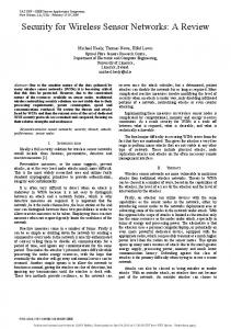
Current architecture for building sensornet applications. An application may choose a subset of network services that it requires. Those network protocols specify a set of link protocols that they support, which constrains the platforms available for application developers. . . . . . . . . . . . . . . . . . The network architecture for many sensornet applications, including environmental monitoring and event detection. . . . . . . . . . . . . . . . . . . . . Packet yield (left), link quality indicator (LQI,center), and received signal strength (RSSI,right) outdoors with the Telos mote and internal antenna. The results are averaged over 10 receivers co-located. From 75-110 feet, a dip in the terrain yields more erratic readings and wider variation in RSSI. Proposed three-tier hardware abstraction architecture. . . . . . . . . . . . . The configuration for the temperature sensor HIL wrapper and how the ADC is exposed with our abstraction. . . . . . . . . . . . . . . . . . . . . . . . . . IEEE 802.15.4 defines two possible network topologies: the star topology (left) and the peer-to-peer topology (right). All networks must have a personal area network (PAN) coordinator. . . . . . . . . . . . . . . . . . . . . . An IEEE 802.15.4 superframe consists of a MAC beacon message followed by a CSMA contention period for other traffic. The duty cycle is bounded by superframe to beacon frame ratio. . . . . . . . . . . . . . . . . . . . . . . In the S-MAC protocol, all nodes within a cell synchronize to a common schedule. Nodes bordering multiple cells must maintain the schedules of all neighboring cells. . . . . . . . . . . . . . . . . . . . . . . . . . . . . . . . . . Interfaces for flexible control of B-MAC by higher layer services. These TinyOS interfaces allow services to toggle CCA and acknowledgments, set backoffs on a per message basis, and change the LPL mode for transmit and receive. . . . . . . . . . . . . . . . . . . . . . . . . . . . . . . . . . . . . . .
2.2 2.3
2.4 2.5 2.6
2.7
2.8
2.9
3
12 13
23 30 35
39
40
41
44
v 2.10 Clear Channel Assessment (CCA) effectiveness for a typical wireless channel. The top graph is a trace of the received signal strength indicator (RSSI) from a CC1000 transceiver. A packet arrives between 22 and 54ms. The middle graph shows the output of a thresholding CCA algorithm. 1 indicates the channel is clear, 0 indicates it is busy. The bottom graph shows the output of an outlier detection algorithm. . . . . . . . . . . . . . . . . . . . . . . . . 2.11 When turning on the radio, the node must perform a sequence of operations. The node first starts in sleep state (a), then wakes on a timer interrupt (b). The node initializes the radio configuration and commences the startup phase of the radio. The startup phase (c) waits for the crystal oscillator to stabilize. Upon stabilization, the radio enters receive mode (d). After the receive mode switch time, the radio enters receive mode (e) and a sample of the received signal energy may begin. After the ADC starts acquisition, the radio is turned off and the ADC value is analyzed (f). With LPL, if there is no activity on the channel, the node returns to sleep (g). . . . . . . . . . . . 3.1
3.2
3.3
3.4
3.5
3.6
3.7
Contour of node lifetime (in years) based on LPL check time and network density. If both parameters are known, their intersection is the expected lifetime using the optimal B-MAC parameters. . . . . . . . . . . . . . . . . Duty cycle is affected by the network density and LPL check interval. Typically used LPL check intervals in B-MAC are depicted. The best check interval is the lowest line at a given network density. . . . . . . . . . . . . . The lifetime of each node is dependent on the check interval and the amount of traffic in the network cell. Each line shows the lifetime of the node at that sample rate and LPL check interval. The circles occur at the maximum lifetime (optimal check interval) for each sample rate. . . . . . . . . . . . . Measured throughput of each protocol with no duty cycle under a contended channel. The throughput of each protocol is affected by the amount of nodes contending for the channel and the overhead of the protocol. B-MAC achieves over 4.5 times the throughput of the standard S-MAC unicast protocol through lower per-packet processing and effective CCA. . . . . . . . . The measured power consumption of maintaining a given throughput in a 10node network. As the throughput increases, the overhead of the SYNC period in S-MAC causes the power consumption to increase linearly. The throughput is the average node bitrate (number of data bytes sent in a 10 second time period) in the 10 node network. . . . . . . . . . . . . . . . . . . . . . . . . The effective energy consumption per byte at node C for a network as shown in Figure 3.7. Each node generates a message every 10 seconds (left) and every 100 seconds (right) consisting of 10 fragments of the size given on the x-axis. . . . . . . . . . . . . . . . . . . . . . . . . . . . . . . . . . . . . . . . X network configuration used for packet fragmentation tests. . . . . . . . .
45
48
60
61
62
66
69
70 71
vi 3.8
Relationship between latency and energy for the B-MAC factored protocol in comparison to S-MAC. Left: The end-to-end latency is a linear function of the number of hops in the network. As the overhead of the MAC protocol increases, so does the slope of the latency. Right: As the latency increases, the energy consumed by both B-MAC and S-MAC decreases. The point illustrated on the B-MAC line is the default configuration as shown in Table 3.2. The point on the S-MAC line is the default S-MAC configuration at 10% duty cycle with adaptive listening. . . . . . . . . . . . . . . . . . . . . . . . 3.9 10 hop configuration used for multihop end-to-end latency tests. . . . . . . 3.10 As the traffic around a node increases, so does the duty cycle when using the B-MAC protocol with LPL. The node one-hop from the base station forwards 85% of the packets in the deployment yet achieves a lower duty cycle by minimizing the preamble length on packets sent to the base station. 3.11 The position in the network dictates the amount of traffic flowing through that level. As we approach the base station, nodes handle an increasing number of packets. The average duty cycle is computed by finding the average for nodes at a given hopcount. Fractional hopcounts are correlated with nodes that oscillated between two levels of the network. Note that the nodes one-hop away from the base station can achieve a lower duty cycle because the base station is always on. By reconfiguring B-MAC to use short packets, nodes one-hop from the base station survive up to 50% longer. . . . . . . . 3.12 The average latency of packets being delivered by the Surge application is dependent on the traffic in the network and reliability of each link. The average exceeds the expected latency because retransmissions add additional latency to each packet. . . . . . . . . . . . . . . . . . . . . . . . . . . . . . . 4.1 4.2
5.1
5.2
5.3 5.4
Conceptual view of SP architecture. Network services interact with various link protocols through the shared SP neighbor table and message pool. . . . The SP send process stores an SP message in the pool, schedules it for transmission, and then requests the next packet in the SP message. Note that all message and packet storage is created by the network service advocating a “pay for what you use” policy. . . . . . . . . . . . . . . . . . . . . . . . . . B-MAC cooperates with SP through an SP adaptor. The adaptor converts primitives and control mechanisms provided by B-MAC into notifications for SP. . . . . . . . . . . . . . . . . . . . . . . . . . . . . . . . . . . . . . . . . . When using 15.4, each node runs the 15.4 protocol and cooperates with SP through the SP adaptor. The adaptor assists in maintaining the neighbor table and waking the radio to listen to surrounding nodes. . . . . . . . . . . The send and receive interfaces used in TinyOS 1.x . . . . . . . . . . . . . . Mapping of link implementations to active messages in TinyOS. From left: Mica stack with RFM TR1000 bit radio, Mica2 stack (B-MAC), and Mica2 stack (S-MAC). The Telos stack with the CC2420 radio (15.4) is identical in composition to the Mica2 B-MAC stack. . . . . . . . . . . . . . . . . . . . .
73 73
75
77
79
85
92
101
105 109
110
vii 5.5
6.1
6.2 6.3 6.4 6.5 6.6 6.7
6.8
7.1 7.2
The Surge application for Telos wires around the AM abstraction to control the properties of the radio, such as setting RF output power and requesting acknowledgments. . . . . . . . . . . . . . . . . . . . . . . . . . . . . . . . . . SP provides neighbor table and message pool structures. The required entries of the SP neighbor table are shown on the left, while the structure of SP messages is shown on the right. . . . . . . . . . . . . . . . . . . . . . . . . . The sp message t data structure for sending packets. . . . . . . . . . . . . The SPSend interface. . . . . . . . . . . . . . . . . . . . . . . . . . . . . . . The default sp neighbor t neighbor table entry. The entry may be expanded by redefining the structure in the header files of other services. . . . . . . . The SPNeighbor interface. . . . . . . . . . . . . . . . . . . . . . . . . . . . . Network protocol offered load versus delivered load of SP running above 15.4 (at 1.5% and 12.5% duty cycles) and B-MAC (using low power listening). . Delivered throughput using the control and feedback mechanisms provided by SP on the Mica2. Each node transmits as quickly as possible. Congestion control (CC) and phase adjustment are implemented at the network layer using SP . . . . . . . . . . . . . . . . . . . . . . . . . . . . . . . . . . . . . . Delivered throughput of a single hop channel running 15.4 at 1.5% and 12.5% duty cycles under congestion. Each node transmits as quickly as possible– more nodes lead to more channel congestion. . . . . . . . . . . . . . . . . . Trickle propagation behavior on 15.4. New data is injected at the lower left corner node with time measured in seconds. . . . . . . . . . . . . . . . . . . Multiple network protocols running above SP can cause the overall system to save power compared to running the protocols independently. This figure shows a two minute excerpt of communications traffic identified by protocol running on the Mica2. The top graph shows an idle node while the bottom graph shows the protocols piggybacking on other messages. MintRoute packets are shown in white and synopsis diffusion packets are gray. . . . . .
110
113 115 116 119 120 125
126
128
144
145
viii
List of Tables 2.1 2.2
2.3 2.4 2.5
3.1
3.2
5.1
7.1
7.2
The family of Berkeley motes and their capabilities. . . . . . . . . . . . . . Microcontroller history: The main table contains traditional microcontrollers; the bottom two devices are 32-bit microprocessors presented for comparison. . . . . . . . . . . . . . . . . . . . . . . . . . . . . . . . . . . . . Capabilities of current COTS radios suitable for WSNs, their features, and power profile. . . . . . . . . . . . . . . . . . . . . . . . . . . . . . . . . . . . Measured current consumption of Telos compared to Mica2 and MicaZ motes A comparison of the size of B-MAC and S-MAC in bytes. Both protocols are implemented in TinyOS. . . . . . . . . . . . . . . . . . . . . . . . . . . . . . Time and current consumption (I) for completing primitive operations of a monitoring application using the Mica2 mote and CC1000 transceiver. Identifiers on each operation map back to the activities of acquiring a radio sample in Figure 2.11. . . . . . . . . . . . . . . . . . . . . . . . . . . . . . . . . . . Parameters for a monitoring application running B-MAC. The first three parameters are specific to Mica2 motes; the next three are default values for B-MAC parameters on the Mica2; the remaining parameters are application semantics affecting the performance of B-MAC. Each parameter affects the total energy consumed by the node, E. . . . . . . . . . . . . . . . . . . . . . Comparison of how two classes of link protocols, sampled and slotted, map to mechanisms present in SP. . . . . . . . . . . . . . . . . . . . . . . . . . . Comparison of the code and memory usage of MintRoute in TinyOS and MintRoute built above the SP abstraction. “Engine” relays multihop messages from the application to the link protocol. “Neighbors” performs neighbor management. RAM is the memory usage, Msgs is the amount of RAM used by message buffers, and Flash is the code size in bytes. . . . . . . . . . Statistics that illustrate the stability and effectiveness of MintRoute running on 29 nodes in a 15.4 network over an eight hour period. . . . . . . . . . . .
15
17 18 25 49
55
56
100
141 142
ix 7.3
8.1 8.2
Measured code size and memory usage for the Trickle and Synopsis Diffusion SP implementations. RAM is the memory usage, Msgs is the amount of RAM used by message buffers, and Flash is the code size in bytes. . . . . . Interaction between SP and link protocols . . . . . . . . . . . . . . . . . . . Network Protocols above SP and their use of the SP neighbor table and message pool. Features marked as helpful indicate where code complexity is reduced if used. . . . . . . . . . . . . . . . . . . . . . . . . . . . . . . . . . .
143 149
156
x
Acknowledgments I owe tremendous gratitude to my parents, Kathleen Benyo and Robert Polastre, and my grandparents, Catherine Molnar, Eleanor Polastre, and Joseph Polastre. Through their constant support, they pushed me to excel both in life and in work. They gave me the drive to accomplish any goal that I set. David Culler dedicated countless time and energy to advise, guide, and transform my ideas into the work presented in this dissertation. David taught me the intricacies of what it means to be a researcher. David has been extremely supportive, no matter how far my ideas strayed during my tenure at Berkeley. He always managed to pull them back in and taught me to frame my ideas in the context of a much larger, more compelling picture. My work at Berkeley improved significantly in quality over time; David often challenged my ideas and assumptions thereby encouraging a deep analysis of every problem. I have grown significantly since I met David, both personally and academically, and I am extremely grateful for his commitment, patience, and teaching. Professors Scott Shenker and Ion Stoica added significant value with their networking experience. Conversations with Scott and Ion forced me to think outside the microcosm of wireless sensor networks. They have always been available to share their wisdom. Few people can tolerate my musings for any extended period of time.
Rob
Szewczyk and Cory Sharp not only supported my randomness, but also became actively involved in it. Rob and Cory are two of my most trusted advisors, both as friends and co-workers. Jonathan Hui has been a co-conspirator in the design, implementation, and eval-
xi uation of SP. Jonathan’s insights were critical for turning SP into a working system from merely a design on paper. Jonathan has been an amazing friend; it has been a pleasure to work with him and I hope that we continue our many amazing conversations in the future. Phil Levis provided feedback on much of the work in this dissertation. His dedication and attention to detail resulted in profound improvements. The networking students at Berkeley, especially Jason Hill, Alec Woo, George Porter, Prabal Dutta, Kamin Whitehouse, and David Molnar, are a world-class group with a constant supply of ideas and amusement. They helped me through the down times with frosty beverage and some encouragement. I am fortunate to have met Jen McGaffey, who has always been around to listen whenever an issue arose. Jen has ushered me into numerous live shows in San Francisco free of charge, shared many beers with me, and helped take my mind off the inevitable frustrations that I encountered during my graduate student career. Finally, this work was supported by a number of funding agencies including: the National Science Foundation under grant #0435454 (“NeTS-NOSS”), DARPA grant F33615-01-C1895 (“Network Embedded Systems Technology (NEST)”), California MICRO, the Center for Information Technology Research in the Interest of Society (CITRIS), the Intel Research Laboratory at Berkeley, and other NSF support.
1
Chapter 1
Introduction The promise of Wireless Sensor Networks (also referred to as sensornets and WSNs) is the ability to sample, coordinate, and actuate at scales and densities not previously possible. Wireless sensors are an enticing tool enabling a wide array of applications. Sensor networks have been used for industrial monitoring, distributed control and actuation, microclimate monitoring, asset tracking, and security. Sensornets have the ability to use the sum of their parts for a common purpose; as the density of a sensornet increases, the potential computational power, storage, and functionality also increases. Each node in a wireless sensor network has limited capabilities, but cooperative processing and communication yields a large distributed network performing the tasks of an application. Tiny sensor nodes can be deployed directly at the point of interest, providing more faithful data about the item under study. There are many challenges when deploying wireless sensor networks. Due to their low cost and constrained size, wireless sensors suffer from a limited power supply and adverse
2 radio conditions. For example, Woo [89] and Zhao [95] independently verified the existence of a “gray region” in radio connectivity where some nodes exceed 90% successful reception while neighboring nodes receive less than 50% of the packets. They shows that the gray area is rather large—one-third of the total communication range. When developing protocols, such as a reliable transport protocol for wireless sensor networks, new mechanisms must be employed to contend with environmental conditions. The gray region is just one of the many networking challenges posed by wireless sensor networks. These challenges have motivated a broad set of investigations over the past decade, which have given us a cornucopia of possible protocols at each level in the network stack. For instance, many different physical links, with widely differing characteristics, have been utilized ([5, 16, 33, 62, 73, 74, 75]). Myriad low power media access protocols have been developed, based either on CSMA ([54, 66, 88]), TDMA ([19, 58, 83, 92]), or both ([28, 59]). In addition, numerous topology formation algorithms ([4, 25, 91]), routing protocols ([52, 89]), aggregation algorithms ([41, 50]), and dissemination protocols ([2, 25, 30, 40]) have been proposed. The resource scarcity of sensornets requires minimizing energy usage while maintaining high reliability and data quality over time-varying and noisy links ([89, 95]). To meet these ambitious goals, most research efforts have emphasized performance more than modularity, with many issues (such as power management, scheduling, and data buffering) handled simultaneously at many levels in a deeply intertwined fashion. As a result, the field has produced a few vertically integrated designs, each with its own interface assumptions, and there is little code reuse.
3
In-Network Storage
Timing
Security
Custody Transfer Discovery
System Mgmt.
Power Mgmt.
Sensornet Application
Address-Free Protocols Suppression
Predicates
Triggers
Name-Based Protocols Caching
Estimation
Graphs
Naming
Sensornet Protocol Data Link Physical Architecture
Media Access Sensing
Timestamping
Energy Storage
Coding
Carrier Sense
Assembly Transmit
ACK Receive
Figure 1.1: Sensornet Functional Layer Decomposition
In response to this inability to compose protocols within a wireless sensing system, many researchers noted the need for a sensornet architecture [8]. Such an architecture would provide much greater modularity to sensornet designs, thereby regularizing assumptions about interfaces, encouraging code reuse, and fostering greater intellectual synergy.1 Moreover, if the architecture has a “narrow waist” (as does the Internet architecture), then it could effectively decouple many aspects of the software from the underlying hardware. Such a decoupling would be of great benefit given the rapid technological advances in the sensornet arena, particularly in radio transceivers. In contrast to the Internet, the narrow waist (which we call the sensornet protocol, SP) should not be at the network layer but should instead sit between the network and link layers. Shown in Figure 1.1, SP facilitates interaction between link protocols and network protocols through a unified interface. This “lowering of the waist” is necessary because processing potentially occurs at each hop, not 1
Zigbee [96] proposes a classic layered architecture, but each layer assumes a specific instance of the surrounding layers; e.g., the routing layer assumes the IEEE 802.15.4 link and physical layers. As standards bodies ratify future revisions of IEEE 802.15.4 and other link protocols, Zigbee must be completely rearchitected to use these technologies. An architecture built on static technologies is destined for obsolescence.
4 just at the end points, and there are many application-specific multi-point communication patterns (collection, aggregation, dissemination, and others). Thus, one cannot base the sensornet architecture around the end-to-end delivery of packets, but instead must build upon the lower-level base of a single-hop data link mechanisms. The key challenge for SP is providing adequate insulation between the hardware below and the various communication abstractions above while not sacrificing efficiency. SP should allow network level protocols to optimize for the underlying link in terms of the cost and performance characteristics expressed at SP, rather than knowing which particular link and physical layer resides beneath.2 Moreover, SP must allow network protocols to choose neighbors wisely, taking into account information available at the link layer. Thus, rather than the strict and opaque layering used in the Internet, we claim SP must be translucent; it must provide enough information so that the network and link layers can cooperate to achieve effective use of communication resources, but it must do so in a way that is independent of the link layer. For SP to be useful, network protocol development should be easy, through a few simple choices rather than a bewildering set of hard-to-configure parameters. Because of limited resources, primarily power, SP must facilitate interaction between system protocols. Coordination and cooperation can significantly reduce power consumption while not sacrificing performance. SP borrows the idea of “flexible interfaces” from existing protocols [54]. Flexible interfaces allow protocols to be reconfigured at runtime by other protocols that have acquired additional information about the the operation of the 2
This is in contrast to IEEE 802.2 [72] which provides a uniform syntactic interface to various link layers, but the code above takes specific actions based on the particular protocol beneath, whether it is ethernet, 802.11, or others.
5 system. For example, a network protocol may recognize end-to-end congestion and instruct the link protocol to sleep until the congestion subsides. Unlike IP, SP provides mechanisms for power-aware communication and facilitates out-of-band communication between protocols on either side of SP. Protocols are developed relative to the unified abstraction and are isolated from the details of underlying link protocols. In this dissertation, we describe our design for SP. We translate the general notion of a decoupling interface for wireless sensor networks into a concrete proposal for a unifying link-level abstraction. Multiple network protocols cooperatively optimize with link protocols through our abstraction. This abstraction is novel in how it promotes cooperation across the link and network layers to utilize limited resources efficiently. Our SP design is simple, giving network layer protocols only one bit to express their desires about the urgency and reliability3 (or importance) of a message. At the same time, it allows link-layers and network protocols to cooperate by maintaining and exposing a shared neighbor table and message pool. Most protocols use a neighbor table and would benefit from a shared structure. The message pool allows all outgoing messages to be scheduled, either by other network protocols or the underlying link. Each of these structures serves as an information sharing mechanism provided by our SP abstraction. These structures fit into the primary theme of this dissertation: the development of mechanisms, primitives, and abstractions that ultimately extend the lifetime of wireless sensor networks. Extending lifetime is typically achieved through two methods: reducing power consumption and increasing robustness. SP must facilitate both of these methods. 3
Reliability refers to a best effort transmission of the message, not a guarantee that it will be received by the intended recipient(s).
6 Reduced power consumption is the result of increased cooperation among protocols. Increased robustness comes with the introduction of a unifying interface that separates the concerns of each protocol. If each protocol only focuses on its mechanisms, then protocol design, implementation, and debugging can be completed quickly and in isolation. Once integrated with the system, SP provides protocols with a rich communication interface. Evaluation of our SP abstraction includes more than just benchmarks and studies of applicability. It takes many years of hard use to evaluate an architecture, since its goal is not to excel in one particular circumstance but instead to perform adequately in a wide range of scenarios. Our design of SP was based on our experience with a variety of link and network protocols, and we have done the thought-experiment of asking how one might use them above and below SP. While these musings were encouraging, they are hardly convincing. To provide more concrete evidence, we report in this dissertation on a smaller set of cases that we have implemented and measured. This dissertation is organized in nine chapters. Chapter 2 establishes a background understanding of key technology that serves as the foundation for building our SP abstraction. The chapter presents the hardware platforms, protocols, and architectures currently in use. We introduce the need for fine-grained software control and system flexibility in wireless sensing systems. All of the components in a sensor network must work together for the system to be efficient, power conscious, and robust. Starting at the bottom and working our way up, we discuss wireless sensor platforms, including the four generations of “motes” from the University of California, Berkeley. Unique hardware techniques and flexible software control present in new motes increase both lifetime and robustness. When
7 writing software that interfaces with the hardware, tension exists between full abstraction and maximum performance. We introduce the concept of “Flexible Hardware Abstraction”, a hierarchy of system abstractions that allow developers to trade off performance for platform independence. Finally, we discuss the two prominent classes of link protocols that must work with our SP abstraction, sampling and slotted, with a representative example for each class, B-MAC and IEEE 802.15.4. Link protocols expose varying degrees of control to network services. In Chapter 3, we introduce B-MAC, a protocol designed with a high degree of flexibility and configuration to yield more efficient systems. The efficiency gain is due to network protocol reconfiguration of the link based on changing conditions. Chapter 3 presents a framework for analyzing the operation of a wireless sensor network application. We present B-MAC to motivate flexible control and translucent layering also found in SP. By building a model, collecting microbenchmarks using different traffic patterns, and evaluating a real-world application, we show that highly flexible interfaces are necessary to control a wireless system for long-lived operation. After motivating the need for flexible software services in wireless sensor networks, Chapter 4 introduces our SP abstraction and establishes the concepts present in a unified link abstraction. Chapter 4 discusses the design decisions that led to the final SP abstraction and primitives that SP provides to link and network protocols for simple yet expressive control. The motivation behind the SP neighbor table, message pool, and control and feedback mechanisms stems from existing protocols and interfaces. By collecting common activities into a single unified interface, SP provides the framework to build a larger sensor
8 network architecture. For SP to be effective, a wide range of link and network protocols must be able to use SP efficiently. Chapter 5 describes how sampling and slotted protocols, specifically B-MAC and IEEE 802.15.4, map their primitives to SP with the help of an SP adaptor. We show the effectiveness of SP through a TinyOS implementation in Chapter 6. We demonstrate that a single implementation of a network protocol yields power-aware operation on links with differing power management strategies. Using microbenchmarks, we evaluate SP relative to the two link protocols from Chapter 5. We prove that SP is just as applicable to single-hop networks as multi-hop networks, making our abstraction applicable regardless of which type of network becomes the predominant type in the future. Ultimately, SP must serve as a unified abstraction for network protocols that can optimize their operation independent of the underlying link. In Chapter 7, we present a multi-hop collection protocol, a dissemination protocol, and an aggregation protocol. Each of these protocols is implemented using SP. We describe their implementation and present a number of benchmarks showing that performance of each protocol did not suffer when using SP. In fact, we show that optimizations fall out naturally by providing a unifying abstraction. We have not seen these optimizations in monolithic approaches or previous work. Finally, we show multiple network protocols gaining mutual benefit by cooperating on a common link abstraction. Our SP abstraction is a first attempt at a unified link protocol that serves as the “narrow waist” in wireless sensor networks. To prove the applicability of SP to other types of protocols, we describe how other link and network protocols could use SP in Chapter 8.
9 Certain aspects that could be part of a link abstraction are not addressed by SP; we present these concepts in Chapter 8, potential changes to SP, and need for maintaining a small set of necessary and sufficient primitives. Chapter 9 concludes this dissertation. We present the implications of having a unified link protocol and the need for its adoption by developers. We conclude with predictions and future work for creating system software using SP and a larger sensor network architecture.
10
Chapter 2
Architectural Composition of Sensornets The promise of wireless sensornets is their ability to tackle problems at scales and densities not possible with traditional wireline technology. Wireless technology must meet the goals of each application subject within the constraints of low energy supplies, low computational power, and noisy radio conditions. In this chapter, we explore the constrains, tensions, and proposed solutions for building each piece of a sensornet application, up to the boundary between data link and network protocols. This chapters describes existing sensornet technology that establishes the multitude of protocols that must be supported and the challenges presented by hardware and data link layers. Figure 2.1 shows the composition of protocols in a sensornet application. Current abstractions limit protocols from cooperating within a system. The layer underneath currently limits the protocols that may be used within that system. In this chapter, we address
11 the difficulty of abstraction in sensornets from the bottom of Figure 2.1, working our way up. Many constraints are placed on software by hardware platforms. The hardware trends and tradeoffs in component and platform selection are discussed in Section 2.1. Hardware design dictates the amount of functionality available to software. Section 2.2 describes the family of “Berkeley motes”, using the Telos platform as a concrete example of concepts that hardware should provide to build efficient software. Section 2.3 presents the system design for controlling hardware through software to achieve application goals, such as interoperability, lifetime, or raw performance. We move up the stack to the link protocols in Section 2.4 and present the two classes of WSN link protocols: slotted and sampled. At each layer, we use existing protocols and abstractions as exemplars that illustrate the importance of cooperation and flexibility between layers instead of strict boundaries. Applications are better equipped to meet lifetime and robustness requirements through flexible use of hardware, link protocols, and network protocols. To show the purpose and interactions that exist at each layer of a sensornet protocol stack, we examine the goals and operation of a wireless monitoring application. By evaluating the needs of the application, we introduce requirements and constraints that the WSN system must address. We examine the integration of hardware and software and present an architecture that promotes flexible control of both hardware and software subsystems. We discuss existing link protocols and their interaction with both the underlying hardware and the network protocols that rely on them. Monitoring applications represent a significant class of sensornet applications. Monitoring takes many forms—environmental and microclimate monitoring, industrial and
12 Tracking Application
Pt-Pt Routing 1-1
Neighborhood Sharing 1-k / k-1
802.15.4
Telos
Aggregation N --- 1
B-MAC
MicaZ
Sensing Application
Data Collection N-1
S-MAC
Mica2
Robust Dissemination 1-N
PAMAS
Dot
Mica
Figure 2.1: Current architecture for building sensornet applications. An application may choose a subset of network services that it requires. Those network protocols specify a set of link protocols that they support, which constrains the platforms available for application developers. building monitoring, home automation, and event detection. To focus our discussion, we look at the goals of a habitat monitoring application and use it to drive the requirements and constraints in our sensornet. We use the class of monitoring applications, all implemented within the framework of Figure 2.2, to illustrate a typical application. Two deployments are used as examples to ground our analysis—the Great Duck Island (GDI) project that monitors elusive seabirds and the California Redwoods project that monitors arboreal microclimates. As described in [43, 53], scientists on GDI are interested in the biologically-significant data, primarily to determine the pattern and conditions under which the Leach’s Storm Petrel breeds. To correlate data and prove hypotheses, the system must survive for the duration of a breeding season, approximately seven months, and reliably report data readings. Similarly, biologists
13
Patch Network
Sensor Node
Sensor Patch
Gateway Transit Network
Client Data Browsing and Processing
Basestation Base-Remote Link
Internet
Data Service
Figure 2.2: The network architecture for many sensornet applications, including environmental monitoring and event detection. studying the California Redwoods [70, 77] are interested in knowing the temporal and spatial microclimate variations that exist within a redwood forest. Their study must also remain operational for several months in order to compare and contrast the microclimate variations and tree physiology across different days and seasons within a redwood grove. Even applications that seem completely different, such as distributed event detection [12], rely on the sensornet to be long-lived and maintain coverage over a large area for extended periods of time. The typical network architecture for wireless sensornet applications is shown in Figure 2.2. This architecture represents the networks deployed on both GDI and in the California Redwoods. For the work presented in this dissertation, we focus on the interaction between nodes within the sensor patch such that the goals of each application are met, such as maximizing coverage and lifetime. Both deployments reinforced important aspects of a sensornet deployment. Ulti-
14 mately, these systems delivered biologically-significant data but also exposed the need for more robust, lower-power hardware and software implementations. We identified areas of improvement that include sensornet management and introspection, the ability to retask the network with new logic or program images, the need to abstract underlying hardware to reuse application logic across deployments, and increased hardware/software integration to mitigate the effect of subsystem failures. Improving any of these areas results in a longer overall system lifetime with more reliable data reporting. From this experience, we conclude that the usefulness of wireless sensornet systems is ultimately driven by lifetime, and lifetime is affected by energy consumption and robustness. Lifetime and energy consumption are themes that drive our work throughout this dissertation. To fully understand the constraints in sensornet systems, we have illustrated the physical network architecture (Figure 2.2) and the node software architecture (Figure 2.1). Applications are composed from a subset of available network protocols. Each of these protocols must optimize their operation based on the demands of the application. Under the current architecture, each platform is only compatible with a subset of available link protocols residing beneath the network protocols. Links must cooperate with network protocols and hardware platforms to yield the best overall performance. Each layer of the software architecture in Figure 2.1 has to resolve the tension between the requirements of upper layers and the primitives provided by lower layers. Our proposed SP abstraction rises to the ask of resolving this tension by exposing the link protocols and hardware to network protocols in a unified manner. In the remainder of this chapter, we discuss existing hardware, link protocols, and abstraction that SP exposes through its unifying abstraction.
15 Mote Type WeC Ren´e Ren´e Dot Mica Mica2Dot∗ Mica2∗ Year 1998 1999 2000 2000 2001 2002 2002 Microcontroller Type AT90LS8535 ATmega163 ATmega128 Program memory (KB) 8 16 128 RAM (KB) 0.5 1 4 Active Power (mW) 15 15 8 33 Sleep Power (µW) 45 45 75 75 Wakeup Time (µs) 1000 36 180 180 Nonvolatile storage Chip 24LC256 AT45DB041B Connection type I2 C SPI Size (KB) 32 512 Communication Radio TR1000 TR1000 CC1000 Data rate (kbps) 10 40 38.4 Modulation type OOK ASK FSK Receive Power (mW) 9 12 29 Transmit Power at 0dBm (mW) 36 36 42 Power Consumption Minimum Operation (V) 2.7 2.7 2.7 Total Active Power (mW) 24 27 44 89 Programming and Sensor Interface Expansion none 51-pin 51-pin none 51-pin 19-pin 51-pin Communication IEEE 1284 (programming) and RS232 Integrated Sensors no no no yes no no no
Telos 2004 TI MSP430 48 10 3 15 6 ST M25P80 SPI 1024 CC2420 250 O-QPSK 38 35 1.8 41 16-pin USB yes
* Based on the Mica mote, these commonly used derivatives are manufactured by Crossbow Technology.
Table 2.1: The family of Berkeley motes and their capabilities.
2.1
Hardware Design and Constraints Each year, new microcontrollers and radio transceivers are released to the market
with varying capabilities. Some are more suitable for low cost, low power wireless sensors than others. The University of California, Berkeley has introduced at least four wireless sensor platforms, called “motes”, that are in widespread use today. Table 2.1 shows these designs, their capabilities, and the trends in wireless hardware capabilities over time. Energy consumption, one of our primary metrics, is defined as the current consumed by an operation multiplied by the time that operation takes to complete. For a low power platform, our goal is to minimize both the time that an operation takes and the cur-
16 rent consumed during that operation. Therefore, we try to reduce sleep current and active current, sleep as much as possible, and have a very short wakeup time when transitioning from sleep to active modes. Individual component selection is not only critical for minimizing the power consumption of each part of the system, but also for controlling the rest of the system. For example, the microcontroller must be able to duty cycle the radio, turn sensors on and off, and shut down peripherals when not in use. These subsystems should be independent and controllable to mitigate the effect of a subsystem failure and finely control energy consumption. Table 2.2 summarizes the microcontroller improvements over time, illustrating the realm of low cost components currently available to wireless sensornet platforms. For microcontrollers, the trend is to keep RAM and Flash sizes nearly constant while adding additional hardware modules; RAM and Flash size for low cost, low power microcontrollers has not significantly increased in the last 30 years. There are a number of approaches to mitigate the impact of limited RAM and Flash. Additional hardware modules, added by many microcontroller manufacturers, reduce load on the main MCU core. Modules and external circuitry may reduce application complexity, lowering RAM and Flash usage, at the cost of increased power consumption. Our applications must be designed to operate within the constraints of limited RAM and Flash. There are two distinct types of low power, low data rate radios: narrowband and wideband radios shown in Table 2.3. Selecting an appropriate transceiver is particularly difficult and depends on the application. The wide array of features yield different power profiles, flexibility available to software, and are not necessarily complimentary.
17 Manufacturer Device Atmel
General Instruments Microchip Intel
Philips Motorola
Texas Instruments Atmel Intel
AT90LS8535 Mega128 Mega165/325/645 PIC
RAM Flash Active Sleep Release (kB) (kB) (mA) (µA) 0.5 8 5 15 1998 4 128 8 20 2001 4 64 2.5 2 2004 0.025 0.5 19 1 1975
PIC Modern 4 4004 4-bit 0.625 8051 8-bit Classic 0.5 8051 16-bit 1 80C51 16-bit 2 HC05 0.5 HC08 2 HCS08 4 TSS400 4-bit 0.03 MSP430F14x 16-bit 2 MSP430F16x 16-bit 10 AT91 ARM Thumb 256 XScale PXA27X 256
128 4 32 16 60 32 32 60 1 60 48 1024 N/A
2.2 30 30 45 15 6.6 8 6.5 15 1.5 2 38 39
1 N/A 5 10 3 90 100 1 12 1 1 160 574
2002 1971 1995 1996 2000 1988 1993 2003 1974 2000 2004 2004 2004
Table 2.2: Microcontroller history: The main table contains traditional microcontrollers; the bottom two devices are 32-bit microprocessors presented for comparison. Narrowband radios typically give software the most control over the radio—they can be started and stopped in a very short period of time and are controlled at the bit or byte level. Many narrowband radios provide very fast startup times since they are clocked by the MCU at the cost of a large software overhead (in the form of interrupts and processing cost) on the MCU. Hill illustrated the benefits of narrowband radios for low power communications in [27] to build an extremely low power link wakeup protocol. Although the protocol Hill describes was low power, it suffered from a high bit-error rate due to the simple encoding scheme provided by the narrowband transceiver. Narrowband radios typically have simple modulation schemes, no spreading codes, and are not robust to noise.
18 Type Vendor Part no. Max Data rate (kbps) RX power (mA) TX power (mA/dBm) Powerdown power (µA) Turn on time (ms) Modulation Packet detection Address decoding Encryption support Error detection Error correction Acknowledgments Interface Buffering (bytes) Time-sync Localization
RFM TR1000 115.2 3.8 12 / 1.5 1 0.02 OOK/ASK no no no no no no bit no bit RSSI
Narrowband Chipcon Chipcon CC1000 CC2400 76.8 1000 9.6 24 16.5 / 10 19 / 0 1 1.5 2 1.13 FSK FSK,GFSK no programmable no no no no no yes no no no no byte packet/byte 1 32 SFD/byte SFD/packet RSSI RSSI
Nordic nRF2401 1000 18 (25) 13 / 0 0.4 3 GFSK yes yes no yes no no packet/byte 16 packet no
Chipcon CC2420 250 19.7 17.4 / 0 1 0.58 DSSS-O-QPSK yes yes 128-bit AES yes yes yes packet/byte 128 SFD RSSI/LQI
Wideband Motorola MC13191/92 250 37(42) 34(30)/ 0 1 20 DSSS-O-QPSK yes yes no yes yes yes packet/byte 133 SFD RSSI/LQI
Zeevo ZV4002 723.2 65 65 / 0 140 * FHSS-GFSK yes yes 128-bit SC yes yes yes packet yes * Bluetooth RSSI
* Manufacturer’s documentation does not include additional information.
Table 2.3: Capabilities of current COTS radios suitable for WSNs, their features, and power profile. In contrast, wideband radios are very robust to noise but give up significant flexibility in the process. Enhanced modulation schemes found in wideband radios, such as spread spectrum (DSSS) and phase shift keying (O-QPSK), provide signal robustness to noise and interference at the cost of higher power consumption. Almost all wideband radios are packet-based and use this feature to transfer at higher data rates than a microcontroller can sustain. Hardware modules may be provided for security and encryption, synchronization, and channel coding. These modules come at a cost; because the radio exposes data to the microcontroller on a packet basis, the microcontroller does not have the fine grained control that existed with narrowband radios. The bit-based protocol described by Hill has much lower energy consumption than the same method running on a packet-based wideband radio like the CC2420. Additional protocol cost is due to the internal complexity of the radio—wideband radios must wait for high speed oscillators to start in order to modulate or decode a wireless signal and must be accessed at a coarser granularity.
19 To pick the most applicable radio, we must evaluate the impact of noise, flexibility available to the end application, ease of communication with other devices, power consumption, startup times, and available data bandwidth. No single radio in Table 2.3 is globally optimal; instead a radio must be chosen based on application requirements.
2.2
Node Design To illustrate how a wireless sensor network platform supports the goals of WSN ap-
plications, we discuss the design and implementation of Telos. Telos is the fourth-generation Berkeley mote that leverages experience with WeC, Ren´e, and Mica platforms (in Table 2.1). Our analysis includes intuition behind hardware selection, and flexibility offered by the Telos platform to software developers in order to build low power, robust systems. The Telos platform is the result of over 12 months of research and development by two full-time graduate students including the author and numerous collaborators at the University of California, Berkeley. Telos is a completely new design based on experiences from using previous mote generations designed by former graduate students at Berkeley and researchers at other institutions (Intel, ETH Zurich, TU Berlin, and others). We designed Telos to meet three major goals: ultra-low power operation, ease of use, and robust hardware and software implementation. The goals of Telos are in line with the requirements outlined earlier in this chapter.
20
2.2.1
Component Selection For Telos, we chose the MSP430 microcontroller after evaluating existing products
from Atmel, Motorola, and Microchip. Table 2.2 shows that the MSP430 has the lowest power consumption in both sleep and active modes. The microcontroller operates down to 1.8V. Low voltages are important for extracting all of the energy out of a power source— e.g., alkaline AA batteries have a cut-off voltage of 0.9V. If two alkaline batteries are used in series, the system cut-off voltage is 1.8V, exactly the same as the minimum required voltage for the MSP430. In contrast, the ATmega128 MCU (Mica family) will only run down to 2.7V, leaving almost 50% of the alkaline batteries unused.1 The MSP430 also has the fastest wakeup time of any microcontroller; transitioning from standby (1µA) to active mode (4-8MHz) in no more than 6µs. Instead of increasing RAM or flash size, microcontroller manufacturers leverage free die space for powerful hardware modules integrated into embedded microcontrollers. The MSP430 has a DMA controller that operates while the MCU core is sleeping. The DMA permits applications to sample from the ADC, output a voltage on the DAC, or transfer data to and from the radio without interrupting the MCU. Through the DMA controller, software can achieve a greater degree of concurrency without sacrificing power. DMA is traditionally used to increase performance, but in the case of low power embedded systems, the DMA controller actually lowers the duty cycle by permitting the MCU core to remain 1
When moving from the Ren´e to Mica platforms, Hill recommended the MSP430 microcontroller due to its low power but ultimately chose the Atmel because it had a larger user base and open-source development tools [26]. Years later, the MSP430 now has open-source tools and large development community making the microcontroller much more feasible for mote designs. Hill describes a follow on to Mica, called “Blue”, that uses the MSP430 in [26]. Although we initially chose a Motorola HCS08 for Telos (which has almost identical characteristics to the MSP430), we dismissed it due to poor code density and a lack of development tools and support.
21 asleep longer and service less interrupts. The performance enhancements of DMA permit up to 200ksamples/sec ADC sampling, compared to a maximum of 10ksamples/sec on MCUs without DMA (some powerful 8-bit and 16-bit MCUs can achieve as high as 70ksamples/sec, but no interrupt-based method on current MCUs can achieve 200ksamples/sec). The limited sampling rate is caused by the overhead of context switching due to interrupts after each ADC conversion. Less interrupt handling and automatic DMA processing yields smaller and simpler code in almost all cases. Telos also has built-in brown-out reset, supply voltage supervisor, and interrupt driven sensors to maximize the sleeping time of the mote while still providing event notifications to software. For Telos, we chose the new IEEE 802.15.4 standard. By using a standardized radio, Telos can communicate with any number of devices sharing the same physical layer, including devices with quite different node architectures and transceiver manufacturers. The primary factor in selecting a radio technology was the desire to experiment with and build on the new IEEE 802.15.4 wireless technology. Telos uses the Chipcon CC2420 radio in the 2.4GHz band, a wideband radio with O-QPSK modulation with DSSS at 250kbps. The higher data rate allows shorter active periods further reducing energy consumption. Previous mote designs emphasized the need for low radio startup times. Duty cycled protocols, such as preamble sampling [27], require quick wakeup (less than one millisecond) to minimize duty cycle. Deployments on Great Duck Island [71] on Mica2 motes and at the Intel Developers Forum [79] on Dot motes were extremely energy starved. In both deployments, idle listening was the primary energy consumer. Idle listening occurs when a node wakes up, listens to the channel, but there is no communication activity. The
22 radio crystal used on Telos was carefully chosen to minimize idle listening; we chose a lowESR 16MHz crystal. Low resistance is essential for minimizing the work required to start a crystal oscillating. The Telos crystal yields a 580µs startup time, almost 300µs lower than the minimum advertised startup time by Chipcon, the manufacturer of the radio. Since IEEE 802.15.4 radio interfaces are packet-based, we lose considerable flexibility in software for controlling the operation of the radio. However, the CC2420 provides a number of hardware modules to achieve better performance. These include encryption and authentication, packet handling support, auto acknowledgments, and address decoding. Since hardware modules are embedded in the radio instead of the microcontroller, the modules may not be used as general purpose functions. For example, an application may want to encrypt a data buffer and store it in flash; however, since the buffer is not being sent over the radio, the hardware encryption module within the radio cannot be used. Other downsides include auto acknowledgment support; when this feature is used, packets not addressed to the local node are discarded by hardware, preventing services from overhearing messages destined for other nodes that are useful for link estimation and routing. An alternate approach to adding hardware modules in the radio is to add hardware accelerators in the microcontroller. Spec, designed by Jason Hill [26], included specialized hardware accelerators that offload MCU intensive portions of RF operations. The design philosophy of Spec was to include only general accelerators that could be composed efficiently by software to provide the full functionality required by a wireless sensor. In contrast to encoding a full networking stack or link protocol in hardware that is currently done by Bluetooth and Zigbee IC manufacturers, Spec retains significant software flexibility while
23
0.8
0.8
0.6
0.4
0
0 100 150 Distance (ft)
200
250
−30
0.4
0.2
50
−20
0.6
0.2
0
−10
RSSI (dBm)
1
Average LQI
Packet Yield (%)
0 1
−40 −50 −60 −70 −80 −90
0
50
100 150 Distance (ft)
200
250
−100
0
50
100 150 Distance (ft)
200
250
Figure 2.3: Packet yield (left), link quality indicator (LQI,center), and received signal strength (RSSI,right) outdoors with the Telos mote and internal antenna. The results are averaged over 10 receivers co-located. From 75-110 feet, a dip in the terrain yields more erratic readings and wider variation in RSSI. decreasing power consumption and MCU processing by an order of magnitude. Hill evaluated each potential hardware accelerator with respect to the potential energy saved and weighed its power benefits against the loss of flexibility that the hardware module imposes. Spec accelerators included interrupt execution acceleration for lightweight RF event handling, a simplified DMA controller for transmission and reception, transmission timing, and data encryption. Beyond hardware accelerators, radios now provide software with metadata about the incoming signal previously only available by accessing the radio at a very low level. For example, the CC2420 radio, as dictated by IEEE 802.15.4, samples the first eight chips of a packet, measures the error in the modulation, and calculates a Link Quality Indicator (LQI) value. We tested the effect of distance on received signal strength (RSSI), packet success rate, and link quality (LQI). We placed 10 receivers at the same location and 1 node transmitting at 0 dBm at a distance d, all located 4” above the ground outdoors. We averaged the results over all receivers. Figure 2.3 shows the average packet success, LQI, and RSSI for Telos using the internal antenna. The LQI provided by the radio closely maps
24 to the packet success rate as shown in Figure 2.3. The RSSI follows an exponential decrease while the packet success rate is high; after 60 feet, the signal is noisier and decreases to the minimum sensitivity of the transceiver. The small variance in RSSI among receivers and the correlation between LQI and packet success rate provides additional information not previously available to network services, such as multihop networking and localization. The hardware, in the case of the CC2420, provides unique information about its operation. Since the hardware does not always know the implications of the metrics that it collects, it is critical that this information is pushed up the network software stack so that other services can optimize accordingly. The consequence of using a higher speed radio is that it may saturate the processing capabilities of the MCU when the channel is fully loaded. We ran experiments on a 30 node Telos network to measure the effective bandwidth. A single Telos node is able to source approximately half of the full data bandwidth of the channel, or 125kbps. When all 30 nodes transmit as quickly as possible, Telos is limited to an average reception rate of 150kbps. Our current implementation is interrupt driven; however, we intend to increase performance by using the DMA controller to directly transfer data from the radio, reduce the number of interrupt context switches, and reduce the number of receive buffer overflow events. The overall energy consumed during a sampling cycle (wakeup, sample, transmit, and sleep) using Telos is lower than existing platforms. The energy consumed is the total time the mote is active multiplied by the current consumption during that time; thus it was important to reduce both startup time and current consumption. If an application samples its sensor and sends data once every three minutes, we estimate Telos can last for almost
25 Operation Minimum Voltage Mote Standby (RTC on) MCU Idle (DCO on) MCU Active MCU + Radio RX MCU + Radio TX (0dBm) MCU + Flash Read MCU + Flash Write MCU Wakeup Radio Wakeup
Telos 1.8V 5.1 µA 54.5 µA 1.8 mA 21.8 mA 19.5 mA 4.1 mA 15.1 mA 6 µs 580 µs
Mica2 2.7V 19.0 µA 3.2 mA 8.0 mA 15.1 mA 25.4 mA 9.4 mA 21.6 mA 180 µs 1800 µs
MicaZ 2.7V 27.0 µA 3.2 mA 8.0 mA 23.3 mA 21.0 mA 9.4 mA 21.6 mA 180 µs 860 µs
Table 2.4: Measured current consumption of Telos compared to Mica2 and MicaZ motes
3 years using standard alkaline AA batteries. For comparison, the estimated lifetime of the Mica2 mote is 1.5 years and the MicaZ mote is 1 year [56]. Further power consumption statistics are provided in Table 2.4
2.2.2
Robustness The previous sections discussed the low power tradeoffs when building a wireless
sensor node, using Telos to illustrate the design space. To extend system lifetime, the sensor platform can employ a number of hardware and software techniques that increase overall system robustness. These techniques focus on flexible control of the system through a synergy of hardware and software. A fundamental low power technique is to isolate each hardware “sub-circuit”. Using simple software routings, power to the circuit can be turned on or off independently from the rest of the platform. In the event of a failure, faulty modules can be disabled to minimize their impact on the system. Two experiences on GDI motivated hardware
26 isolation. First, the initial GDI deployment used the Mica platform with a 3.3V boost converter. The converter maintained a stable system voltage to support uniform radio operation and range. The boost converter consumed a significant amount of current, even when the mote was asleep. To extend the lifetime of the node, we bypassed the boost converter with a diode, permitting the node to run directly from the battery when asleep. We envisioned that future revisions could turn the boost converter on or off when needed. On Telos, the CC2420 includes its own LDO voltage converter that maintains a stable 1.8V supply for the radio. The LDO may be turned on or off through software on the microcontroller. Second, one of the main predictors of node failure in the GDI deployment was the existence of a failed sensor [69]. Since the failure can be recognized in software, the ability to cut power to that section of the board may have saved the system as a whole. Subsystem isolation also enables fine-grain control over power consumption of the system at runtime. Only the components necessary for carrying out current operations are active, with all others disabled. For example, the sensors on Telos may be disconnected by software running on the microcontroller. Telos also prevents current from leaking back into the USB circuitry by isolating USB components when hardware detects that the USB port is no longer connected to a PC. Another technique for increased robustness is protected storage. Hardware writeprotection for system flash is essential for wireless reprogramming—a known good program image may be stored in write-protected flash. By controlling the write-protection through hardware, there is always a fallback mechanism to a usable application. Based on expe-
27 riences with the California Redwoods and ExScal [12] deployments, we noticed that we could not recover a node quickly if it was wirelessly reprogrammed with a faulty program. Telos introduced hardware write-protection that guarantees the mote always has a good program image available for recovery. When plugged into a USB port, the write-protection is disabled and the first segment of the external flash may be written. When running on batteries (without USB), the segment is write-protected. Deluge [30] is an epidemic code-propagation protocol used in BNP [29] to reprogram the network wirelessly. Deluge and BNP take advantage of hardware write-protection. In the event that a faulty code image renders the node unusable, a halted node may be reset via the watchdog timer or a button (referred to as a “Golden Gesture”). Telos will automatically reload the code flash in the microcontroller with the hardware protected golden image.
2.2.3
Software Integration There is a huge impact on the software when creating a new hardware platform.
TinyOS [39] is a componentized operating system suitable for research in wireless embedded systems. In TinyOS, composition of fine-grained components to build an application allows researchers to work on the system at any level (e.g., the details of hardware device drivers and link protocols up to the application semantics). The MSP430 architecture is significantly different from the microcontrollers commonly used in TinyOS. We were forced to rethink hardware abstraction for embedded systems. Many of the abstractions in TinyOS focused on the Atmel family of microcontrollers. Because of their specificity, we were unable to extract adequate performance from
28 the MSP430 or access all of the rich hardware modules in the MSP430. TinyOS lacked arbitration mechanisms (such as acquiring or releasing a hardware bus by multiple device drivers) and hardware-independent control of isolated subsystems within a platform. The emergence of Telos created an opportunity to redesign the existing TinyOS 1.1.x interfaces. Overall, the goal was to create effective abstractions that take advantage of the powerful hardware features of the MSP430 microcontroller while providing abstraction to the application developer. As a first attempt at cross-platform development in TinyOS, we built a platformindependent radio stack (link protocol and physical layer access) for the CC2420 transceiver. Each platform using the CC2420 implements a set of components that provide register access to the radio; the radio stack then acts as a library that uses the hardware-independent wrappers to control the radio. Our CC2420 implementation operates on Telos, MicaZ, iMote2, and Chipcon CC2420EB platforms. Since these platforms all share the same physical layer, TinyOS enables cross-platform communication and research on hybrid networks. The CC2420 two-layer approach has a number of drawbacks, but motivated the development of a full architecture for power efficient yet hardware-independent resource use in embedded systems.
2.3
System Abstractions The previous section showed that reconfiguration and flexibility of hardware com-
ponents is essential for low power systems. Unfortunately, traditional hardware abstraction either completely hides the details of the underlying hardware or sacrifices performance.
29 Since energy is a scarce resource, applications must be able to use hardware efficiently by trading off abstraction for efficiency when needed. This problem led us to develop a new abstraction architecture for wireless sensornets that provides an additional degree of flexibility. We developed a three-tier architecture shown in Figure 2.4 to provide a hardware independent abstraction regardless of microcontroller or radio. Our architecture addresses the tension between abstraction and efficiency through its three-layer approach. We chose to expose the primitives of the hardware, such as register access and module flags, through a hardware presentation layer (HPL). A platform-dependent hardware adaptation layer (HAL) exposes module functionality so that the full power of the hardware may be used. Example HAL functions include getting data from the ADC, setting a hardware timer, or writing to external flash. The hardware independent layer (HIL) exposes a subset of the capabilities of a platform that are available to system services, sacrificing efficiency for performance where required to meet uniform interfaces across platforms. The capabilities of the underlying hardware are gradually adapted to the established platform-independent interface between the operating system and the applications. As we move from the hardware towards this top interface, the components become less and less hardware dependent, giving the developer more freedom in the design and implementation of reusable applications. The HPL/HAL/HIL model is implemented in TinyOS for the TI MSP430 microcontrollers and has been adopted as the basic architecture for hardware abstraction by the TinyOS 2.0 Working Group.
30
Cross-platform applications
Platform-specific applications
Platform-specific applications Platform-independent hardware interface
HIL 1
HIL 2
HIL 3
HAL 2 HAL 1
HAL 3
HIL 4
HAL 4
HPL 1
HPL 2
HPL 3
HPL 4
HW Platform 1
HW Platform 2
HW Platform 3
HW Platform 4
HW/SW boundary
Figure 2.4: Proposed three-tier hardware abstraction architecture.
2.3.1
Hardware Presentation Layer (HPL) The components belonging to the HPL are positioned directly over the HW/SW
interface. As the name suggests, their major task is to “present” the capabilities of the hardware using the native concepts of the operating system. They access the hardware in the usual way, either by memory or by port mapped I/O. In the reverse direction, the hardware can request servicing by signaling an interrupt. Using these communication channels internally, the HPL hides the hardware intricacies and exports a more usable interface (simple function calls) for the rest of the system. The HPL components should be stateless and expose an interface that is fully determined by the capabilities of the hardware module that is abstracted. This tight coupling
31 with the hardware leaves little freedom in the design and the implementation of the components. Even though each HPL component will be as unique as the underlying hardware, all of them will have a similar general structure. To integrate with the rest of the architecture, each HPL component should have:
• commands for initialization, starting, and stopping of the hardware module that are necessary for effective power management policy • “get” and “set” commands for the register(s) that control the operation of the hardware • separate commands with descriptive names for the most frequently used flag-setting and flag-testing operations • commands for enabling and disabling of the interrupts generated by the hardware module • service routines for the interrupts that are generated by the hardware module
Interrupt service routines in the HPL components perform only the most timecritical operations (like copying a single value, clearing flags, and disabling the module), and delegate the rest of the processing to the higher level components that possess extended knowledge about the state of the system. Our HPL structure eases manipulation of the hardware. Instead of using cryptic macros and register names whose definitions are hidden deep in the header files of compiler libraries, the programmer can now access hardware through a familiar interface.
32 This HPL does not provide any substantial abstraction over the hardware beyond automating frequently used command sequences. Nonetheless, it hides the most hardwaredependent code and opens the way for developing higher-level abstraction components. These higher abstractions can be used with different HPL hardware-modules of the same class. For example, many of the microcontrollers used on the existing WSN platforms have two USART modules for serial communication. They have the same functionality but are accessed using slightly different register names and generate different interrupt vectors. The HPL components can hide these small differences behind a consistent interface, making the higher-level abstractions resource independent. The programmer can then switch between the different USART modules by simple rewiring (not rewriting) the HPL components, without any changes to the implementation code.
2.3.2
Hardware Adaptation Layer (HAL) The adaptation layer components represent the core of the architecture. They use
the raw interfaces provided by the HPL components to build useful abstractions hiding the complexity naturally associated with the use of hardware resources. In contrast to the HPL components, they are allowed to maintain state that can be used for performing arbitration and resource control. Due to the efficiency requirements of WSN, abstractions at the HAL level are tailored to the concrete device class and platform. Instead of hiding the individual features of the hardware class behind generic models, HAL interfaces expose specific features and provide the “best” possible abstraction that streamlines application development while maintaining effective use of resources.
33 For example, rather than using a single “file-like” abstraction for all devices, we propose domain specific models like Alarm, ADC channel, and EEPROM. According to our model, HAL components should provide access to these abstractions via rich, customized interfaces, and not via standard narrow ones that hide all the functionality behind a few overloaded commands.
2.3.3
Hardware Interface Layer (HIL) The final tier in our architecture is formed by the HIL components that take
the platform-specific abstractions provided by the HAL and convert them to hardwareindependent interfaces used by cross-platform applications. These interfaces provide a platform independent abstraction over the hardware that simplifies the development of the application software by hiding the hardware differences. To be successful, this API “contract” should reflect the typical hardware services that are required in a WSN application. The complexity of the HIL components mainly depends on how advanced the capabilities of the abstracted hardware are with respect to the platform-independent interface. When the capabilities of the hardware exceed the current API contract, the HIL “downgrades” the platform-specific abstractions provided by the HAL until they are leveled-off with the chosen standard interface. Consequently, when the underlying hardware is inferior, the HIL might have to resort to software simulation of the missing hardware capabilities. As newer and more capable platforms are introduced in the system, the pressure to break the current API contract will increase. When the performance requirements outweigh the benefits of the stable interface, a discrete jump will be made that realigns the API with the abstractions provided in the newer HAL. The evolution of the platform-independent inter-
34 face will force a reimplementation of the affected HIL components. For newer platforms, the HIL will be much simpler because the API contract and their HAL abstractions are tightly related. On the other extreme, the cost of boosting up (in software) the capabilities of the old platforms will rise. Since we expect HIL interfaces to evolve as new platforms are designed, we must determine when the overhead of software emulation of hardware features can no longer be sustained. At this point, we introduce versioning of HIL interfaces. By assigning a version number to each iteration of an HIL interface, we can design applications using a legacy interface to be compatible with previously deployed devices. This is important for WSNs since they execute long-running applications and may be deployed for years. An HIL may also branch, providing multiple different HIL interfaces with increasing levels of functionality.
2.3.4
Selecting the Level of Abstraction The platform-dependence of the HAL in our architecture leads to the more general
question about why we have opted for a three-layered design. In other words, why we did not expose the platform-independent hardware interface directly from the HAL components. The main reason behind our decision is the increased flexibility that arises from separating the platform-specific abstractions and the adaptation wrappers that upgrade or downgrade them to the current platform-independent interface. In this way, for maximum performance, the platform specific applications can circumvent the HIL components and directly tap to the HAL interfaces that provide access to the full capabilities of the hardware module. Selecting the “right” level—whether an application should use the HIL or directly
35
Figure 2.5: The configuration for the temperature sensor HIL wrapper and how the ADC is exposed with our abstraction. access the HAL—can sometimes cause one hardware asset to be accessed using two levels of abstraction from different parts of the application or the OS libraries. For example, take an application similar to the standard OscilloscopeRF application in TinyOS. The application uses the ADC to sample several values from a temperature sensor and sends them in the form of a message over the radio. If the observed phenomenon does not have a large signal bandwidth and the time between subsequent conversions is long, for the sake of cross-platform compatibility, the programmer might decide to use the standard ADCHILSingle interface. This interface is exported by the HIL sensor wrapper (Figure 2.5) using the services of the platform-specific HAL component. When enough samples are collected in the message buffer, the application passes the message to the networking stack. The MAC protocol used for message exchange over the radio uses clear channel assessment to determine when it is safe to send the message. This usually requires taking several samples of the RSSI signal provided by the radio hardware. Since this is a very time critical operation in which the correlation between the consecutive samples has a significant influence, the programmer of the MAC might directly use the MSP430ADC12Multiple in-
36 terface of the HAL component as it provides much finer control over the conversion process. As a result of this chain of decisions, we end up with a concurrent use of the ADC hardware module using two different levels of abstraction. To support this type of “vertical” flexibility we include more complex arbitration and resource control functionality in the HAL components. HAL components handle arbitration between multiple services simultaneously access the resources exported by the HPL.
2.3.5
Summary Sensornet applications primarily require long lifetimes and robust operation. These
requirements map down to hardware and software constraints that wireless technology must meet: low cost, low power, and constrained flash and RAM sizes. We have shown hardware trends over the past 30 years and their impact on wireless sensor network platforms. Flash size, memory, and power consumption remain fairly constant. To reduce the demands of software, many vendors have introduced new powerful hardware modules such as DMA controllers and advanced ADC processing. Software must take advantage of these modules while maintaining fine-grained control over power consumption. WSN solutions must employ a high degree of flexibility, such as hardware subsystem isolation and abstraction at multiple levels, in order to achieve long lifetimes and mitigate the effect of failed subsystems. For software to run efficiently on these platforms, it is crucial that the hardware may be reconfigured and disabled. To achieve efficient service implementations, we introduced a three-tier hardware abstraction architecture. Services may now choose the level of abstraction most suited to their application while still achieving high efficiency and low power consumption.
37 These services are not limited to lower level implementations. In the ensuing sections, specifically Section 2.4.1 and Section 2.4.2, we show that link protocols must optimize in terms of the underlying hardware. Accordingly, network protocols then optimize to the link. This process cascades until we have composed a complete application. We continue our discussion by describing link protocols built on existing hardware, their primitives, and their operation.
2.4
Wireless Link Protocols for Sensor Networks The novel constraints of wireless sensor networks—particularly,
energy
conservation—have led to many proposed protocols for media access control (MAC). These protocols fall into two basic classes: slotted protocols and sampling protocols. In slotted protocols, nodes divide time into discrete intervals (slots) and schedule whether the radio is in receive mode, transmit mode, or powered off in terms of these slots. Synchronizing slots with neighbors allows nodes to only power the radio on when needed, significantly reducing idle listening. Slotted protocols are often rigid; after they establish a schedule, a node can usually only communicate with other nodes on the same schedule. Short communication periods can lead to increased contention, plus synchronization maintenance costs both power and bandwidth. Slotted protocols include the TDMA family of protocols [35, 61, 21, 67], IEEE 802.15.4 [75], S-MAC [92], T-MAC [83] and TRAMA [58]. The second class, sampling protocols, takes a different approach. Rather than coordinate time slots, nodes periodically wake up and only start receiving data if they detect channel activity. Depending on the underlying physical layer, this detection can either be
38 based on channel energy or successful symbol decoding. Periodic channel sampling allows a node to conserve energy by keeping its radio off most of the time. In contrast to slotted protocols, sampling protocols are very flexible: a node can communicate with any other node within its radio range. Flexibility comes with a cost, however. Unlike slotted protocols that send regular data packets, sampling protocols must send long, expensive messages to wake up a neighbor. Examples of sampling protocols include Aloha with preamble sampling [13], B-MAC [54], WiseMAC [15], the Chipcon CC2500 transceiver [6], and the Berkeley Mica platform [27]. In this section, we discuss two representative protocols of each class to build a framework and terminology of link protocols used to evaluate our SP abstraction later. For a slotted protocol, we chose IEEE 802.15.4 on the Telos [55] platform; for a sampling protocol, we chose the standard TinyOS Mica2 [80] networking stack (B-MAC on top of the Chipcon CC1000 radio [54]).
2.4.1
Slotted Protocols: IEEE 802.15.4 and S-MAC IEEE 802.15.4 [75], hereafter referred to as “15.4”, was standardized in 2003 to
enable low data rate, low power wireless networking. The protocol supports both star and peer-to-peer topologies depicted in Figure 2.6, with the logic for building those topologies residing above 15.4 at the network layer. 15.4 defines two types of devices that may participate in the network: Full Functionality Devices (FFDs) and Reduced Functionality Devices(RFDs). FFDs may communicate with any other node in the network and may become a network coordinator. RFDs may only communicate directly with a coordinator. A coordinator organizes other nodes in the network. RFDs must associate with a
39
Star Topology
Peer Topology
coordinator
coordinator
Reduced Functionality Device Full Functionality Device
Figure 2.6: IEEE 802.15.4 defines two possible network topologies: the star topology (left) and the peer-to-peer topology (right). All networks must have a personal area network (PAN) coordinator. coordinator in both star and peer topologies. FFDs may associate and communicate with other coordinators, but nodes are not allowed to associate with non-coordinators or RFDs. Each time a coordinator wakes up, it sends out a network beacon. The beacon lets other nodes know the time that it is awake, known as the superframe duration, and the next time a beacon will be sent, known as the beacon duration. The frame structure is shown in Figure 2.7. After receiving a beacon from a coordinator, other devices may synchronize to the the schedule of the coordinator and request to associate. Following notification from the coordinator that the association was successful, associated nodes may send data to the coordinator after its beacon. In the other direction, coordinators advertise data they have for associated nodes in the payload of their beacon message. Nodes may then request data from the coordinator, who then sends the data. For low-latency or periodic data, nodes my request a guaranteed time slot (GTS) from the coordinator. When the coordinator sends out
40
Beacon
Data
Ack
Data
Beacon
CSMA Contention Period
sleep Superframe Duration
Beacon Frame Duration
Figure 2.7: An IEEE 802.15.4 superframe consists of a MAC beacon message followed by a CSMA contention period for other traffic. The duty cycle is bounded by superframe to beacon frame ratio. its beacon, it will indicate which slots after the beacon are “contention-free” and assigned to requesting nodes. The coordinator is responsible for managing and assigning GTS, with support from network protocols. In the peer-to-peer case, FFDs must listen to beacons from other nodes to communicate with them. These nodes must maintain some sort of synchronization, but the measures that need to be taken to achieve synchronization are beyond the scope of the 15.4 standard [75]. The 15.4 standard also describes which operations are the responsibility of the PHY and MAC. The PHY is responsible for turning on and off the radio transceiver, detecting energy on the channel, calculating a the link quality of a packet, selecting channels, and performing clear channel assessment (CCA). The PHY also transmits and receives packets across the physical medium. The PHY is specified at 2.4GHz, 916MHz, and 868MHz. The PHY makes available its energy detection value, link quality indicator, and clear channel assessment. For example, the energy detector may be used to find a clear frequency or
41
Schedule 1
Schedule 2
Figure 2.8: In the S-MAC protocol, all nodes within a cell synchronize to a common schedule. Nodes bordering multiple cells must maintain the schedules of all neighboring cells. channel while the link quality indicator may be used to select the next hop node when routing a packet. Therefore, it is important that these metrics are exposed to the layers above the PHY and MAC so that network protocols can make informed decisions and optimize their operation. The MAC provides primitives to support the star and peer-to-peer network topologies standardized by 15.4. These include the association, disassociation, beaconing, and GTS mechanisms described earlier. The MAC also provides commands for requesting reliable single hop transfer through the use of acknowledgments and hooks for implementing application-specific security mechanisms on a per-link basis. S-MAC is similar to 15.4 with some notable differences in its mechanisms. We use S-MAC in many tests to prove the feasibility and need for translucent layering provided by SP. S-MAC [92] is a low power RTS-CTS scheme for wireless sensor networks inspired by PAMAS [66] and 802.11. S-MAC periodically sleeps, wakes up, listens to the channel, and then returns to sleep. S-MAC is designed to operate like a “black box”—it is optimized for a representative set of workloads. S-MAC does not have any hooks to change its duty cycle or reconfigure its parameters; instead, it combines link, routing, organization, synchronization,
42 and fragmentation services into a single protocol. All of these services may be used by network protocols. Chapter 3 shows how the black box approach of S-MAC hinders specific types of network traffic by trying to perform internal optimizations without knowledge of network protocol activity. In the power management scheme in S-MAC, each active period is of fixed size, 115 ms, with a variable sleep period. The length of the sleep period dictates the duty cycle of S-MAC. At the beginning of each active period, nodes within a cell exchange synchronization information. In contrast to 15.4, each cell maintains a single synchronization schedule instead of each node maintaining its own unique schedule as shown in Figure 2.8. Nodes that can hear more than one cell must maintain synchronization information for all neighboring cells in order to sustain connectivity. An S-MAC active period is broken up into two parts: the first segment is devoted to synchronization (SYNC) and the second segment for data transmissions using CSMA and RTS-CTS. Following the synchronization period, data may be transferred for the remainder of the active period using RTS-CTS. In a follow up paper [93], the authors add adaptive listening—when a node overhears a RTS or CTS packet from a neighbor, it wakes up for a short period of time at the end of the transmission to immediately transmit its own data. Adaptive listening will extend the length of an active period if there is additional data to send by continually waking up at the end of each RTS-CTS exchange and retrying data transmission. Adaptive listening in S-MAC allows S-MAC to achieve lower latency when relaying multihop traffic. By changing the duty cycle, S-MAC can trade energy for latency. S-MAC uses fragmentation to deliver each piece of a message. Fragmentation uses
43 the RTS-CTS scheme to reserve the channel, then transmit packets in a burst. As the size of the network increases, S-MAC must maintain an increasing number of schedules of surrounding nodes or incur additional overhead through repeated rounds of resynchronization. T-MAC [83] improves on the energy usage of S-MAC by using a very short listening window at the beginning of each active period. After the SYNC section of the active period, there is a short window to send or receive RTS and CTS packets. If no activity occurs in that period, the node returns to sleep. By changing the protocol to have an adaptive duty cycle, T-MAC saves power at a cost of reduced throughput and additional latency. T-MAC, in variable workloads, uses one fifth the power of S-MAC. In homogeneous workloads, T-MAC and S-MAC perform equally well. T-MAC suffers from the same complexity and scaling problems of S-MAC. Shortening the active window in T-MAC reduces the ability to snoop on surrounding traffic and adapt to changing network conditions.
2.4.2
Sampling Protocols: B-MAC In contrast to the synchronized 15.4 protocol, B-MAC is a CSMA-based protocol
for wireless sensornets. B-MAC, Berkeley Media Access Control, is motivated by the needs of monitoring applications. It has carefully designed interfaces that allows other services and applications to flexibly control the operation of B-MAC. These services include, but are not limited to, target tracking, localization, triggered event reporting, and multihop routing. Classical MAC protocols perform channel access arbitration and are tuned for good performance over a set of workloads thought to be representative of the sensornet applications. S-MAC is an example of a wireless sensornet protocol designed using a classical
44 interface command command command command command }
MacControl { result_t EnableCCA(); result_t DisableCCA(); result_t EnableAck(); result_t DisableAck(); void* HaltTx();
interface MacBackoff { event uint16_t initialBackoff(void* msg); event uint16_t congestionBackoff(void* msg); } interface command command command command command command command command }
LowPowerListening { result_t SetListeningMode(uint8_t mode); uint8_t GetListeningMode(); result_t SetTransmitMode(uint8_t mode); uint8_t GetTransmitMode(); result_t SetPreambleLength(uint16_t bytes); uint16_t GetPreambleLength(); result_t SetCheckInterval(uint16_t ms); uint16_t GetCheckInterval();
Figure 2.9: Interfaces for flexible control of B-MAC by higher layer services. These TinyOS interfaces allow services to toggle CCA and acknowledgments, set backoffs on a per message basis, and change the LPL mode for transmit and receive. approach. To achieve low power goals and workload requirements, S-MAC is not only a link protocol, but also network and organization protocol. Applications and services must rely on policies internal to S-MAC to adjust operation as node and network conditions change; such changes are opaque to the application. In contrast, the B-MAC protocol contains a small core of media access functionality. B-MAC uses clear channel assessment (CCA) and packet backoffs for channel arbitration, link layer acknowledgments for reliability, and low power listening (LPL) for low power communication. B-MAC is only a link protocol, with network services like organization, synchronization, and routing built above its implementation.
signal (dBm)
45 80 90
100
Outlier
Threshold
110
0
20
40
60
80
100
0
20
40
60
80
100
0
20
40
60
80
100
1 0
1 0
Time (ms)
Figure 2.10: Clear Channel Assessment (CCA) effectiveness for a typical wireless channel. The top graph is a trace of the received signal strength indicator (RSSI) from a CC1000 transceiver. A packet arrives between 22 and 54ms. The middle graph shows the output of a thresholding CCA algorithm. 1 indicates the channel is clear, 0 indicates it is busy. The bottom graph shows the output of an outlier detection algorithm. Although B-MAC does not provide multi-packet mechanisms like hidden terminal support or message fragmentation and does not enforce a particular low power policy, has a set of interfaces that allow services to tune its operation (shown in Figure 2.9) in addition to the standard message interfaces2 . These interfaces allow network services to adjust the mechanisms provided by B-MAC, including CCA, acknowledgments, backoffs, and LPL. By exposing a set of configurable mechanisms, protocols built on B-MAC make local policy decisions to optimize power consumption, latency, throughput, fairness or reliability. For effective collision avoidance, a MAC protocol must be able to accurately determine if the channel is clear, referred to as Clear Channel Assessment (CCA). Since the ambient noise changes depending on the environment, B-MAC employs software automatic 2 Standard interfaces for message transmission in TinyOS [81] are BaseSendMsg for transmission, ReceiveMsg for reception, and RadioCoordinator for time stamping and start of frame delimiter (SFD) information.
46 gain control for estimating the noise floor. Signal strength samples are taken at times when the channel is assumed to be free—such as immediately after transmitting a packet or when the data path of the radio stack is not receiving valid data. Samples are then entered into a FIFO queue. The median of the queue is added to an exponentially weighted moving average with decay α. The median is used as a simple low pass filter to add robustness to the noise floor estimate. An α value of 0.06 and FIFO queue size of 10 provided the best results for a typical wireless channel. Once a good estimate of the noise floor is established, a request to transmit a packet starts the process of monitoring the received signal from the radio. A common method used in a variety of protocols, including 15.4, takes a single sample and compares it to the noise floor. This thresholding method produces results with a large number of false negatives that lower the effective channel bandwidth. Since noise has significant variance in channel energy whereas packet reception has fairly constant channel energy (as shown in Figure 2.10), B-MAC searches for outliers in the received signal such that the channel energy is significantly below the noise floor. If an outlier exists during the channel sampling period, B-MAC declares the channel is clear since a valid packet could never have an outlier significantly below the noise floor. If five samples are taken and no outlier is found, the channel is busy. The effectiveness of outlier detection as compared to thresholding on a trace from a CC1000 [5] transceiver is shown in Figure 2.10. The most basic mechanism allows services to turn CCA on or off using the MacControl interface in Figure 2.9. By disabling CCA, a scheduling protocol may be implemented above B-MAC. If CCA is enabled, B-MAC uses an initial channel backoff when sending a packet. B-MAC does not set the backoff time, instead an event is signaled
47 to the service that sent the packet via the MacBackoff interface. The service may either return an initial backoff time or ignore the event. If ignored, a small random backoff is used. After the initial backoff, the CCA outlier algorithm is run. If the channel is not clear, an event signals the service for a congestion backoff time. If no backoff time is given, again a small random backoff is used. Enabling or disabling CCA and configuring the backoff allows services to change the fairness and available throughput. B-MAC provides optional link-layer acknowledgment support. If acknowledgments are enabled, B-MAC immediately transfers an acknowledgment code after receiving a unicast packet. If the transmitting node receives the acknowledgment, an acknowledge bit is set in the transmission message buffer of the sender. B-MAC duty cycles the radio through periodic channel sampling that we call Low Power Listening (LPL). Our technique is similar to preamble sampling in Aloha [13] but tailored to different radio characteristics. Each time the node wakes up, it turns on the radio and checks for activity. If activity is detected, the node powers up and stays awake for the time required to receive the incoming packet. After reception, the node returns to sleep. If no packet is received (a false positive), a timeout forces the node back to sleep. Accurate channel assessment (CCA) is critical to achieving low power operation with this method. We use the noise floor estimation of B-MAC not only for finding a clear channel on transmission but also for determining if the channel is active during LPL. False positives in the CCA algorithm (such as those caused by thresholding) severely affect the duty cycle of LPL due to increased idle listening. To reliably receive data, the preamble length is matched to the interval that the
48 30
25
(a)
(b)
sleep
init radio
(d) (e)
(c) radio crystal startup
(f)
(g)
µc rx adc sleep
Current (mA)
20
15
10
5
0
0
0.5
1
1.5
2
2.5
3
Time (ms)
Figure 2.11: When turning on the radio, the node must perform a sequence of operations. The node first starts in sleep state (a), then wakes on a timer interrupt (b). The node initializes the radio configuration and commences the startup phase of the radio. The startup phase (c) waits for the crystal oscillator to stabilize. Upon stabilization, the radio enters receive mode (d). After the receive mode switch time, the radio enters receive mode (e) and a sample of the received signal energy may begin. After the ADC starts acquisition, the radio is turned off and the ADC value is analyzed (f). With LPL, if there is no activity on the channel, the node returns to sleep (g). channel is checked for activity. If the channel is checked every 100 ms, the preamble must be at least 100 ms long for a node to wake up, detect activity on the channel, receive the preamble, and then receive the message. Idle listening occurs when the node wakes up to sample the channel and there is no activity. The interval between LPL samples is maximized so that the time spent sampling the channel is minimized. The check interval and preamble length are examples of parameters exposed through LowPowerListening interface of B-MAC in Figure 2.9. The transmit mode corresponds to the preamble length and the listening mode corresponds to the check interval. We provide a selection of eight different modes (corresponding to 10, 20, 50, 100, 200, 400, 800, and 1600ms for the check interval). Protocols may also set their own preamble length and check interval through the interface. A trace of the power consumption while sampling the channel on a Mica2 mote [80]
49 Protocol B-MAC B-MAC w/ B-MAC w/ B-MAC w/ B-MAC w/ S-MAC
ACK LPL LPL & ACK LPL & ACK + RTS-CTS
ROM 3046 3340 4092 4386 4616 6274
RAM 166 168 170 172 277 516
Table 2.5: A comparison of the size of B-MAC and S-MAC in bytes. Both protocols are implemented in TinyOS. is shown in Figure 2.11. The process in Figure 2.11 applies to essentially any MAC protocol for sensornets. It performs initial configuration of the radio (b), starts the radio and its oscillator (c), switches the radio to receive mode (d), and then performs the actions of the protocol. As a result, the cost for powering up the radio is the same for all protocols. The difference between protocols is how long the radio is on after it has been started and how many times the radio is started. In sensornets, each node typically runs a single application. Since the RAM and ROM available on sensor nodes are extremely limited, keeping the size of the MAC implementation small is important. Reducing the complexity of the protocol reduces state and the likelihood of race conditions. We implemented B-MAC in TinyOS [39] to evaluate its efficacy in meeting our goals. Since B-MAC does not have the RTS-CTS mechanism or synchronization requirements of S-MAC3 , the implementation is both simpler and smaller as shown in Table 2.5. B-MAC does not hinder efficient implementation of network protocols; above B-MAC we implemented an RTS-CTS scheme and a message fragmentation service using the control interfaces provided by B-MAC that have equivalent functionality to S-MAC RTS-CTS and fragmentation services. 3 All tests with S-MAC were performed with the implementation in tinyos-1.x/contrib/s-mac/ in the TinyOS CVS repository [81] as of March 30, 2004.
50
2.5
Summary Wireless sensor networks are built from small microcontrollers and radios, each
with resource constraints and low power profiles. Protocols and application software must be able to cooperatively control other aspects of the system, including both underlying hardware and software. In this chapter, we presented the hardware, hardware abstractions, and link protocols that make up the bottom half of a network stack for sensornets. The situation in sensornets is akin to personal computers; a wide variety of hardware may be combined to create a platform that meets the goal of a class of applications. With the proliferation of hardware, there is a tension between platform-independent abstractions and raw performance. Our hardware abstraction architecture is a solution to accessing hardware resources. Link protocols are built on our hardware abstraction with two drastically different approaches. One synchronizes nodes in the network and the other wakes up surrounding nodes on demand. Both of these protocols and the wide array of hardware underneath must be supported by a unifying link abstraction. Supporting such a wide range of protocols and platforms has the same tension found in our hardware abstraction architecture—the tension between platform-independent abstractions and raw performance. The challenge is to build SP such that services can efficiently use link protocols without knowing the implementation underneath or hindering performance. The remainder of this dissertation focuses on mechanisms to build a unifying abstraction that does not significantly sacrifice performance. The next chapter introduces
51 and analyzes flexible link control, a technique that motivates translucent layers rather than strict opaque layering. Translucent layering passes additional metadata between layers in addition to data packets. Like our hardware abstraction architecture that showed how flexible selection of the level of abstraction is necessary for building applications and device drivers, translucent layering is another technique for increasing efficiency without integrating layers together. In the follow on chapters, we refine the need for flexibility in sensornets and develop an abstraction that enables efficient application design on the platforms and protocols described in this chapter.
52
Chapter 3
The Case for Flexible Link Control Our design of a unifying abstraction, SP, focuses on translucent layering instead of traditional opaque layering. By bridging link and network protocols, SP has the challenge of addressing network protocol needs efficiently while presenting underlying resources in a unified manner. A proposal for flexible control of a link protocol was initially introduced by B-MAC and encourages translucent layering to cooperation closely with network protocols. Translucent layering passes information, such as control parameters and feedback data, from the lower layers to the upper layers and vice versa through interfaces provided by SP. In this chapter, we advocate the need for network services to control underlying link protocols. Unlike traditional networking with Ethernet or IEEE 802.11, many wireless sensor network protocols present a control interface, such as those provided by B-MAC in Figure 2.9, in addition to a data interface. The control interfaces assists optimization of link operation for minimum power consumption or maximum performance. Control is exposed through setting parameters and feedback events that are necessary for efficient operation.
53 Information passing among the link and network layers creates a tension between local optimizations by the link protocol and reconfiguration by network protocols. In Chapter 2 we showed how flexible hardware abstraction led to efficient and robust systems. These same principles motivate link protocol design and operation. Software requires fine grained control over the hardware in order to minimize overall power consumption and enforce local policies. Likewise, network protocols must cooperate with the link in order to optimize transmissions and receptions based on the current traffic pattern. By factoring the link protocol into its primitive components, network protocols may tune link parameters. Different protocols support different traffic patterns, such as low rate data reporting, bulk reliable transfer, and data dissemination. By relying on network protocols for link policy decisions, each type of traffic can be realized individually instead of relying on black-box link protocols designed to execute reasonably well over a number of representative traffic workloads. In this chapter, we present a framework for analyzing the operation of a wireless sensornet application. We use the B-MAC link protocol as a motivating example of flexible link control. We build an analytical model for monitoring applications, such as GDI and the California Redwoods described in Chapter 2, that use B-MAC. The model allows us to calculate and set parameters in B-MAC to optimize the overall power consumption of the application. Using our model, we illustrate the effect of variables not maintained or controlled by the link, such as duty cycle, network density, and sampling rate. Through a series of microbenchmarks, we show the benefits of a factored approach compared to traditional black-box approaches. These benchmarks also illustrate the performance gains
54 a black-box approach can achieve if it exposed control and feedback interfaces for network protocols. Through a separation of concerns, network protocols implemented above B-MAC focus on what they do best—implement and execute network functionality. We conclude this chapter by analyzing a real world monitoring application called Surge. The performance of Surge, its power consumption, and its reliability proves the applicability of our approach to real world system and motivates further use of translucent layering.
3.1
Modeling Lifetime Creating a model of the operation of B-MAC permits network protocol developers
and application users to calculate the expected lifetime of a sensornet system. As we previously discussed in Chapter 2, lifetime is crucial for monitoring applications and relies on the robust, low power operation of each sensor node. By building a model for BMAC, the power of a factored, flexible approach is illustrated by varying the parameters provided by B-MAC. As network conditions change, such as a decrease in the number of neighboring nodes, nodes can react by reconfiguring the link, thereby increasing resilience to environmental changes. We discuss the effect of changing link parameters through the model presented in this section. We model a periodic sensing application (such as GDI [43]) that streams sensor data to a base station. Table 3.1 lists the primitive operations performed by a low power monitoring application and the observed costs when using a CC1000 transceiver. These operations describe a representative class of radios for wireless sensornets. Radios with similar properties are manufactured by Chipcon, Infineon, and Motorola and were presented
55 Operation Initialize radio (b) Turn on radio (c) Switch to RX/TX (d) Time to sample radio (e) Evaluate radio sample (f) Receive 1 byte Transmit 1 byte Sample sensors
Time 350E-6 1.5E-3 250E-6 350E-6 100E-6 416E-6 416E-6 1.1
(s) trinit tron trx/tx tsr tev trxb ttxb tdata
I (mA) 6 crinit 1 cron 15 crx/tx 15 csr 6 cev 15 crxb 20 ctxb 20 cdata
Table 3.1: Time and current consumption (I) for completing primitive operations of a monitoring application using the Mica2 mote and CC1000 transceiver. Identifiers on each operation map back to the activities of acquiring a radio sample in Figure 2.11. in Table 2.3. We use the notation and values in Table 3.1 throughout the remainder of this chapter. The lifetime of a node is determined by its overall energy consumption. If the lifetime is maximized, then the total energy consumption must be minimized, assuming a fixed energy supply. All of the energies, E, are defined in units of millijoules per second, or milliwatts. Calculating the total energy usage can be done by multiplying E by the node lifetime tl . For wireless sensornet applications, the energy used by a node consists of the energy consumed by receiving, transmitting, listening for messages on the radio channel, sampling data, and sleeping.
E = Erx + Etx + Elisten + Ed + Esleep
(3.1)
Sensors are an integral part of wireless sensornets and must be considered when calculating the lifetime of a node. Sampling sensors is often expensive and affects the lifetime of the node. The sampling parameters (shown in Table 3.1) are based on an application deployed by Mainwaring et. al. [43]. In their application, each node takes 1100 ms to start its
56 Notation csleep Cbatt V Lpreamble Lpacket ti n r tl
Parameter Sleep Current (mA) Capacity of battery (mAh) Voltage Preamble Length (bytes) Packet Length (bytes) Radio Sampling Interval (s) Neighborhood Size (nodes) Sample Rate (packets/s) Expected Lifetime (s)
Default 0.030 2500 3 271 36 100E-3 10 1/300 -
Table 3.2: Parameters for a monitoring application running B-MAC. The first three parameters are specific to Mica2 motes; the next three are default values for B-MAC parameters on the Mica2; the remaining parameters are application semantics affecting the performance of B-MAC. Each parameter affects the total energy consumed by the node, E. sensors, sample, and collect data. The data is sampled every five minutes, or r = 1/(5 ∗ 60). The energy associated with sampling data, Ed , is
td = tdata × r Ed = td cdata V
(3.2)
The energy consumed by transmitting, Etx , is simply the length of the packet with the preamble times the rate packets are generated by the application.
ttx = r × (Lpreamble + Lpacket )ttxb Etx = ttx ctxb V
(3.3)
For a periodic application running the B-MAC LPL protocol with a uniform sampling rate, the node will detect and receive data when each of its n neighbors transmit a packet, regardless of the destination. We refer to the density of neighbors surrounding a
57 node as the neighborhood size of the node. Although receiving data from neighbors shortens node lifetime, it allows services to snoop on the channel and make local decisions based on channel activity. We can bound the total time the node will spend receiving based on the neighbor size and establish an upper bound on the energy consumed by receiving, Erx .
trx ≤ nr(Lpreamble + Lpacket )trxb Erx = trx crxb V
(3.4)
Thus far, our analysis has only considered a single wireless cell. To analyze a multihop application, we need to account for the routing traffic through each node due to its children and the children of its neighbors. Instead of r packets per second flowing through a particular node, the traffic through the node must also include all the packets routed by the node and its neighbors. The function children(i) is defined by the multihop routing protocol and is not maintained by B-MAC.
r×
n X
(children(i) + 1)
i=0
Up to this point, our model has been independent of the MAC protocol in use. The MAC protocol is responsible for minimizing idle listening time, tlisten . In B-MAC, idle listening occurs whenever the B-MAC LPL mechanism samples the channel for activity but no activity is present. In order to reliably receive packets, the LPL check interval, ti , must be less than the time of the preamble. Therefore we have the constraint:
58
Lpreamble ≥ dti /trxb e Given a check interval and associated preamble length, we can calculate the time spent sampling the channel. From Figure 2.11, the power consumption of a single LPL radio sample is 17.3µJ. The total energy spent listening to the channel each second, when no activity is present, is the energy of a single channel sample times the channel sampling frequency.
Esample = 17.3µJ = tlisten × clisten tlisten = (trinit + tron + trx/tx + tsr ) × Elisten ≤ Esample ×
1 ti
1 ti
(3.5)
The energy consumed by idle listening when no activity is present is at most the energy consumed by sampling. If a packet is detected when sampling, the node stays awake and may dismiss scheduled sampling points since the node is already awake. When a node is awake and actively receiving, the node incurs less idle listening energy consumption, Esample and instead consumes energy due to receptions, Erx . Finally, the node must sleep for the remainder of the time. The sleep time, tsleep , is simply the time remaining each second that is not consumed by other operations.
tsleep = 1 − trx − ttx − td − tlisten Esleep = tsleep csleep V
(3.6)
59 The lifetime of the node, tl , is dependent on the total energy consumed, E, and the battery capacity, Cbatt . We must bound the lifetime by the available capacity of the battery.
tl =
Cbatt × V × 60 × 60 E
(3.7)
By solving the system of equations (3.1 through 3.6) and entering the parameters in Table 3.2, we can compute energy consumption of each node for a given network configuration. Lifetime may be estimated at compile time, or calculated for a discrete set of values at runtime. Runtime analysis provides reconfiguration feedback to network services before the service commits to a change in link operation.
3.2
Adaptive Control In a typical deployment, scientists will determine the physical location of the nodes
(which affects the neighborhood size of each node, n) and the ideal sampling rate, r. With this information, we can calculate the parameters to attain the best lifetime that B-MAC can achieve. This also provides the scientist with an estimate for how long the network will survive. If we fix the sample rate and vary the network density, n, we can evaluate the effect of neighbors on node lifetime. Solving the system of equations previously presented with the sample rate equal to once every five minutes yields Figure 3.1. Taking a few slices across the figure at realistic check intervals is shown in Figure 3.2. To find the best LPL check interval for an application, locate the expected neighborhood size on the x-axis of
60
180
25
0.
160 140
5
0.
120
75
1
1.25 1.5
80
0.
100
2 2.5
Channel Activity Check Interval (ms)
200
60 40 20 0
0
20
40
60
Neighborhood size
80
100
Figure 3.1: Contour of node lifetime (in years) based on LPL check time and network density. If both parameters are known, their intersection is the expected lifetime using the optimal B-MAC parameters. Figure 3.2 and move up the y-axis to the lowest line. The check interval corresponding with this line will yield the maximum lifetime. For example, a check interval of 50 ms is optimal for a neighborhood size of 20, but if the neighborhood size is only 5, a check interval of 100 ms is optimal. The size of the neighborhood affects the amount of traffic flowing by each node. B-MAC trades off idle listening for a reduced time to transmit and receive. Both the 10-node and 100-node densities are realistic parameters that a node may encounter in its lifetime. A neighborhood size of 10 nodes is common for deployed monitoring applications (such as [69]) whereas a 100 node neighborhood exists when the nodes are packaged in a box and are retasked with a new program image just before shipping to a customer. Due to
61 0.1
200ms check interval 100ms check interval 50ms check interval 25ms check interval 10ms check interval
Effective duty cycle (%)
0.09 0.08 0.07 0.06 0.05 0.04 0.03 0.02 0.01 0
0
20
40
60
Number of neighboring nodes
80
100
Figure 3.2: Duty cycle is affected by the network density and LPL check interval. Typically used LPL check intervals in B-MAC are depicted. The best check interval is the lowest line at a given network density. volatile links and non-uniform power consumption across the network, nodes must closely monitor their neighborhood and shift expensive operations to more capable nodes to extend overall system lifetime. Almost all protocols either maintain neighbor state (link, organization, and routing protocols are a few examples) or can benefit from it if provided by another service. Although B-MAC relies on neighborhood information for optimal power consumption, it relies on other services to provide neighborhood statistics instead of duplicating that functionality within the link protocol. If we fix the neighborhood size to exactly 10 neighbors per node, the optimum LPL check interval changes with sample rate. Increasing the sample rate increases the amount of traffic in the network (just as increasing the neighborhood size also increases the traffic
62 4 3.5
1−min sample period 5−min sample period 10−min sample period 20−min sample period
Lifetime (years)
3 2.5 2 1.5 1 0.5 0
0
50
100
Check Time (ms)
150
200
Figure 3.3: The lifetime of each node is dependent on the check interval and the amount of traffic in the network cell. Each line shows the lifetime of the node at that sample rate and LPL check interval. The circles occur at the maximum lifetime (optimal check interval) for each sample rate. in a periodic application). As a result, each node overhears more packets. We must find the optimal check interval ti such that the lifetime tl is maximized. Lowering the value of ti also lowers the preamble length. The time to transmit and receive a packet is shorter and the radio is sampled more often. The tradeoff of more frequently checking the radio in order to shorten the packet transmission time is shown in Figure 3.3. Notice that the penalty for more idle listening than required by the traffic pattern, left of the maximum lifetime point in Figure 3.3, is much more severe than the penalty for sending packets that are longer than necessary. Figure 3.3 motivates the need for network services to maintain neighborhood state to prevent B-MAC
63 from operating left of the optimal configuration. Our model shows that it is advantageous to change the parameters of the MAC protocol based on changing network conditions. Since sensor networks consist of low power volatile nodes, links will appear or disappear over time [89, 95]. Nodes may join and leave the network, or the size of the neighborhood will change due to changes in the physical environment. The MAC protocol must be able to adjust for these changes and optimize its power consumption, latency, and throughput to support the network services that rely on it. Using our analytical model, the node may recompute the check interval and preamble length. To address reconfiguration, we chose not to implement the functionality in the MAC protocol as Woo and Culler [88] have done. Instead, we created a set of bidirectional interfaces presented in Figure 2.9 that allow network services to change the MAC protocol based on their current operating conditions. By factoring out more complex parts of conventional MAC protocols, services can decide which situations warrant the use of additional control. For example, link layer acknowledgment support in B-MAC may be selected on a per-packet basis. When an acknowledgment fails, services may choose to retransmit the packet, change the destination of the packet, or reconfigure the LPL parameters. One scheme implemented above B-MAC is an RTS-CTS channel acquisition protocol. On each packet transmission, an RTS packet is sent. A CTS response is sent if the destination node is idle and not delaying due to other transmissions. The RTS and CTS packets are sent using LPL. Once the channel is acquired, data and acknowledge packets are sent immediately with CCA and LPL disabled. After acknowledgment, both nodes
64 re-enable LPL and CCA, then they return to sleep. There are numerous other examples of network services that can realize more efficient operation by building on top of a flexible MAC protocol. Multihop routing can benefit from the LPL interface with the following proposal for controlling B-MAC. When a packet is sent to a parent, it is sent with a long preamble. Immediately following the long preamble message, the child sends the remainder of the packets in its queue to its parent with short preambles. By controlling the preamble length, the multihop protocol can amortize the cost of the long preamble over the sequence of messages. This optimization is possible because the service knows that its parent is awake and that there are pending messages in its queue. We analyze optimizations like the aforementioned multihop routing example throughout this chapter and show how flexibility, control, and feedback yield efficient solutions. The benchmarks used in this chapter to analyze flexible link control are repeated in Chapter 6 to show the impact of inserting our SP abstraction between network protocols and B-MAC.
3.3
Effectiveness of Flexible Link Control We examine the effectiveness of flexible link control through a combination of
microbenchmarks that illustrate the impact of each parameter and a microbenchmark that shows the operation of a deployed application. Each protocol is run through a set of simple workloads forming an empirical characterization of protocol performance. The purpose of these microbenchmarks is to show how WSN protocols react to typical wireless conditions— high contention, low to high throughput, low to high latency, and their correlation with power consumption. We contrast the use of RTS-CTS and message fragmentation services
65 implemented above B-MAC using its interfaces to the same mechanisms that are part of the S-MAC protocol. These microbenchmarks build an understanding of how a real application would perform. To validate our model of B-MAC, we look in detail at the performance of a deployed monitoring application that uses B-MAC. We show that the flexibility and information sharing provided as part of the B-MAC protocol allows the multihop routing service and application to make optimizations not possible with opaque layering protocols like S-MAC (described in Section 2.4.1). We show the benefits that S-MAC gains through inspection and configuration by network protocols if it were reimplemented as a flexible protocol with translucent layering. We compare the actual node duty cycles with those predicted by our model and show that our empirical characterizations apply to real world applications.
3.3.1
Single-hop Analysis In this section we use a variety of microbenchmarks to show how functionality
provided by B-MAC may be used effectively. These benchmarks show the effect of a wide array of network conditions on the energy consumption of B-MAC, S-MAC, and T-MAC. We show the potency of the interfaces in B-MAC for building efficient applications and communications protocols. We illustrate the need to configure B-MAC based on the traffic, latency, reliability, and power requirements of network services. The results of the microbenchmarks empirically characterize the performance of B-MAC, providing insight on the expected behavior of B-MAC in real world applications. By examining the performance of B-MAC compared to S-MAC with and without opaque layering, we validate flexible link control as a necessary mechanism for low power, robust wireless sensors.
66
Throughput (bps)
14000
12000
1 0.9
0.8
0.7
10000
0.6
8000
0.5
6000
0.4
0.3
4000
0.2
2000
0
Percentage of Channel Capacity
B−MAC B−MAC w/ ACK B−MAC w/ RTS−CTS S−MAC unicast S−MAC broadcast Channel Capacity
16000
0.1
0
5
10
Number of nodes
15
0 20
Figure 3.4: Measured throughput of each protocol with no duty cycle under a contended channel. The throughput of each protocol is affected by the amount of nodes contending for the channel and the overhead of the protocol. B-MAC achieves over 4.5 times the throughput of the standard S-MAC unicast protocol through lower per-packet processing and effective CCA. Channel Utilization Channel utilization is a traditional metric for MAC protocols that illustrates protocol efficiency. High channel utilization is critical for delivering a large number of packets in a short amount of time. In sensornets, quickly transferring bulk data typically occurs in network reprogramming or extracting logged sensor data. By minimizing the time to send packets, we can also reduce the network contention. In network reprogramming, the network is woken up and reprogrammed as quickly as possible. To find the channel utilization under congestion, we placed n nodes equidistant from a single receiver. Each node transmitted as quickly as possible with the MAC protocol providing collision avoidance. We
67 increased the offered load by adding transmitters. There is no node or radio duty cycling in this test. The throughput achieved by B-MAC and S-MAC is shown in Figure 3.4. In general, better throughput is attained with fewer nodes trying to saturate the channel. With one transmitter, B-MAC outperforms S-MAC broadcast mode (RTS-CTS disabled) by 2.5 times and S-MAC unicast mode (RTS-CTS enabled) by 4.5 times. BMAC outperforms S-MAC for broadcast traffic due to more sophisticated CCA and lower preamble overhead. B-MAC separates out management and policy from the link primitives implementation, allowing each subsystem to be optimized independently and then combined through control interfaces. For unicast traffic, S-MAC suffers from the overhead of RTS-CTS exchanges. Instead of using control messages like RTS-CTS for hidden terminal avoidance, B-MAC allows higher layer services to implement hidden terminal avoidance based on their traffic patterns. For example, after sending a multihop message, all nodes in the cell should refrain from transmitting until two packet times have elapsed to allow the parent (and grandparent) to retransmit up the tree. Changing operation based on the type of message overheard is shown by [88] to be more efficient than control messages for transmitting multihop traffic. Since each type of traffic has different assumptions, letting the originator of the traffic decide the policy for backoffs, rate control, and bandwidth usage can effectively prevent collisions and congestion without the use of costly control messages. To illustrate the effectiveness of a configurable MAC protocol for sensornets, we implemented the RTS-CTS scheme described in Figure 3.2. This scheme illustrates one method that a network service may employ to mitigate the hidden node problem and increase fairness with B-MAC on a per-message granularity. Since B-MAC can utilize 2.5
68 times more of the channel using the CCA algorithm from Section 2.4.2, the RTS-CTS implementation using B-MAC actually provides double the throughput of S-MAC. When many nodes compete for the channel, B-MAC with RTS-CTS support provides identical performance to S-MAC. By separating out the concerns of the MAC protocol from the network service, implementors can focus on each piece independently. Our tests show that this separation does not hinder protocol performance; instead, the separation yields more improves overall performance. Of course, S-MAC could be modified to achieve the same performance as the factored approached. Even with these changes, S-MAC still does not permit varying network protocols, each with optimizations for their own traffic, to co-exist above the MAC protocol.
Energy vs. Throughput We designed B-MAC to run at both low and high data rates configured by network services relying on it. Low duty cycle applications typically have extremely low network throughput to conserve power; however, some application services, such as bulk data transfer that wirelessly reprograms the firmware of a node, stress the high throughput functionality of the MAC protocol for short periods of time. To evaluate how increased throughput affects power consumption, we vary the transmission rate of 10 nodes in a single cell. We bound the latency such that all data in the test must arrive within 10 seconds. For B-MAC, the optimal check interval ti is measured for the traffic pattern, the test is run, and the energy consumption is calculated. For S-MAC, the optimal duty cycle is calculated for the traffic pattern such that the data arrives within the 10 second period. The results are shown in Figure 3.5.
69
Power consumed (mW = mJ/second)
50
B−MAC S−MAC Always On
45
40
35
30
25
20
15
10
5
0
0
50
100
150
Throughput (bits/second)
200
250
Figure 3.5: The measured power consumption of maintaining a given throughput in a 10node network. As the throughput increases, the overhead of the SYNC period in S-MAC causes the power consumption to increase linearly. The throughput is the average node bitrate (number of data bytes sent in a 10 second time period) in the 10 node network. At low data rates, S-MAC can use an extremely low duty cycle to transmit and receive data. As the amount of data increases, so must the duty cycle of S-MAC. When the duty cycle increases, there are more active periods each with a dedicated SYNC period. Due to the overhead of the SYNC period at the beginning of each wakeup, the S-MAC energy consumption increases linearly. In B-MAC, at low throughput we send long preambles with a long check interval ti . Because of the tradeoff between idle listening and packet length, the preamble overhead dominates the energy consumption. The overhead of LPL is mitigated by a more frequent check interval when the throughput exceeds 45 bits per second. Note that the power consumption of B-MAC below 45 bits per second is within 25% of S-MAC;
70
0.4
0.3 0.25 0.2 0.15 0.1 0.05 0
B−MAC w/ no frag control B−MAC w/ frag control S−MAC T−MAC (simulated) Optimal Schedule
0.35
Energy per byte (mJ/byte)
0.35
Energy per byte (mJ/byte)
0.4
B−MAC w/ no frag control B−MAC w/ frag control S−MAC T−MAC (simulated) Optimal Schedule
0.3 0.25 0.2 0.15 0.1 0.05
0
50
100
150
Fragment size (bytes)
200
250
(a) 10 second message generation rate
0
0
50
100
150
Fragment size (bytes)
200
250
(b) 100 second message generation rate
Figure 3.6: The effective energy consumption per byte at node C for a network as shown in Figure 3.7. Each node generates a message every 10 seconds (left) and every 100 seconds (right) consisting of 10 fragments of the size given on the x-axis. however, B-MAC has significantly less state and no synchronization requirements. Services using B-MAC may easily reconfigure the link protocol to change the check interval based on the network bandwidth whereas services using S-MAC must force it to create a new schedule and resynchronize. Figure 3.5 shows that S-MAC actually consumes less power than B-MAC at low traffic loads if it were reconfigurable. We advocate modifying S-MAC to use network protocol cues, such as offered bandwidth, for greater agility at runtime to enable S-MAC to achieve its best performance.
Fragmentation Small periodic data packets are the most common workload in sensornets, but certain cases arise where larger transfers are needed. S-MAC supports large message fragmentation within the MAC protocol using an RTS-CTS exchange for channel reservation.
71 To compare B-MAC directly to the S-MAC goal of efficient message fragmentation, we devised an experiment to match those done by the authors of S-MAC in [93]. Using the network configuration in Figure 3.7, we transmitted packets from sources A and B to sinks D and E by routing through C.
A
E
C
B
D
Figure 3.7: X network configuration used for packet fragmentation tests.
As in [93], our test sent 10 fragments per message. We varied the fragment size and measured the energy consumed for that transfer. C is the energy bottleneck node in the test network—C will cease operation before any other node since it must both receive and relay packets. We evaluate the energy required to deliver the fragments with S-MAC running at 10% duty cycle with adaptive listening. B-MAC is configured with the default parameters from Table 3.2. Figure 3.6(a) shows the energy cost per byte at node C when a message (consisting of 10 fragments) is sent every 10 seconds. Figure 3.6(b) shows the energy cost per byte when the message generation interval is once every 100 seconds. B-MAC without fragmentation control is simply the B-MAC protocol with the default parameters. Each fragment is an independent packet with a long preamble. Due to the flexibility of B-MAC, a fragmentation service built above B-MAC could adjust the MAC protocol settings since it knows the future traffic pattern for delivering its data. In
72 the measurements with fragmentation control, a message fragmentation service is built using interfaces provided by B-MAC in Figure 2.9. The first fragment of the message is sent with LPL enabled and extra bytes to inform the receiver of the number of fragments. The remaining fragments are sent with LPL disabled. After the last fragment, the sender and receiver reenable LPL. With this flexibility, we achieve significant power savings and efficiency essentially identical to S-MAC without the additional overhead of RTS-CTS messages, synchronization messages, and RAM and ROM usage. When the message transmission period is large (as in Figure 3.6(b)), the overhead of S-MAC is readily apparent; the energy consumption per byte of both S-MAC and T-MAC is greater at all fragment sizes than B-MAC with fragmentation support. Figure 3.6 shows that the energy cost of breaking up a short message into even shorter fragments is so high in all of our protocols that it is simply not a viable option in sensornets.
Latency The authors of S-MAC argue that when the MAC protocol is permitted by network services to increase latency, S-MAC can reduce duty cycle and conserve energy. A test for evaluating end-to-end latency was devised in [93]. We reproduced their test to provide a direct comparison between B-MAC and S-MAC. The test is run on a 10-hop network shown in Figure 3.9. In each test, the source node sends 20 messages with a payload of 100-bytes. There is no fragmentation on any message. The latency of B-MAC and S-MAC increases linearly with network depth. When duty cycling is disabled, the effect of RTS-CTS exchanges in S-MAC results in a much steeper slope than B-MAC. For low power communications, B-MAC has a slope almost
73
3000
2500
B−MAC S−MAC Always On
500 450 400
2000 Energy (mJ)
Latency (ms)
550
B−MAC no sleep B−MAC 100ms check B−MAC 100ms check /w ACK S−MAC no sleep S−MAC 10% adaptive
1500
1000
350 300 250 200 150 100
500
50 0
0
2
4
6
8
Number of Hops
(a) End-to-end latency
10
0
0
2
4
Latency (s)
6
8
10
(b) Effect of latency on energy consumption
Figure 3.8: Relationship between latency and energy for the B-MAC factored protocol in comparison to S-MAC. Left: The end-to-end latency is a linear function of the number of hops in the network. As the overhead of the MAC protocol increases, so does the slope of the latency. Right: As the latency increases, the energy consumed by both B-MAC and S-MAC decreases. The point illustrated on the B-MAC line is the default configuration as shown in Table 3.2. The point on the S-MAC line is the default S-MAC configuration at 10% duty cycle with adaptive listening. Source 11
Sink 10
9
3
2
1
Figure 3.9: 10 hop configuration used for multihop end-to-end latency tests.
identical to S-MAC with adaptive listening; however, a lower overall base latency. Since the first packet cannot be sent until an S-MAC active period, it is delayed by at most 1150 milliseconds. Due to the adaptive listening mechanism of S-MAC described in Section 2.4.1, S-MAC does not incur an expected 1150 milliseconds additional delay at each hop. One protocol feature of B-MAC, link layer acknowledgments, increases latency by an insignificant amount.
74 To better evaluate the effect of increasing the latency to reduce power consumption, we fixed the throughput to one 100 byte packet per 10 second interval. We measured the end-to-end latency of the 10 hop network and varied the duty cycle of S-MAC. We also chose the optimal ti for B-MAC given the latency and throughput. The results are shown in Figure 3.8(b). For latencies under 6 seconds, B-MAC performs significantly better than S-MAC. As S-MAC approaches the 10 second latency limit, its power dips below B-MAC. When the latency exceeds 3 seconds, power consumed by B-MAC is bounded by the cost of idle listening. In contrast, the best case performance of S-MAC shown in Figure 3.8(b) relies on S-MAC synchronizing the entire 10-hop network and using adaptive listening to transmit the data through the network in one active period. Figure 3.8(b) shows the importance of reconfiguration in wireless sensornets. If the required latency of the application is relaxed, S-MAC could achieve lower energy consumption than B-MAC; however S-MAC operates at a single setting, is not reconfigurable, and thus cannot realize these energy savings. Figure 3.8(b) illustrates the need for reconfiguration, both at runtime and at compile time. Providing latency control assists network services relying on the link protocol for optimizations. Even though the S-MAC implementation is opaque—network protocols treat it like a black box—Figure 3.8(b) proves that by changing the parameters of S-MAC, and even resynchronizing the network, results in lower overall energy consumption while still meeting the needs of higher layer services.
75 3
1 hop from base station
Duty Cycle (%)
2.5
2
1.5
1
Leaf nodes
0.5
0
0
0.5
1
1.5
2
2.5
Number of packets forwarded or sent
3
3.5 4
x 10
Figure 3.10: As the traffic around a node increases, so does the duty cycle when using the B-MAC protocol with LPL. The node one-hop from the base station forwards 85% of the packets in the deployment yet achieves a lower duty cycle by minimizing the preamble length on packets sent to the base station.
3.3.2
Multihop Analysis The application model early in this chapter predicts the performance of a mon-
itoring application for wireless sensornets using the B-MAC protocol. In this section, we examine the behavior of a real-world monitoring application called Surge. We examine the duty cycle of Surge and compare the results to predictions from the analytical model. The empirical characterizations from Section 3.3.1 are evaluated with the networking results from Surge. We also examine the use of the interfaces provided by B-MAC for simple optimizations that have a large impact on the lifetime of the network. Surge is a periodic data collection application that acquires samples from sensors,
76 sends its readings, and sleeps. The Surge application is almost identical to application used on GDI with the exceptions noted in this section that take advantage of flexible link control. It was deployed by uniformly placing 14 nodes throughout a 30 meter by 20 meter home. The nodes automatically configured themselves into an ad-hoc routing network. Surge collects data from each node once every three minutes. Instead of collecting sensor data, we acquired statistical information from B-MAC about its performance. For each node, Surge transmits the energy usage, battery voltage, link quality to surrounding nodes, and the parent selected. Data from Surge is used to verify that the network performance matches the data from Section 3.3.1. Using our estimate of lifetime versus check interval for a given sample period (see Figure 3.3), we selected a 100ms check interval ti . By evaluating the node communication range and overall size of the network, we expected a maximum neighborhood size of 5 nodes. To be conservative, we calculated the preamble length and check interval with a neighborhood size of 10. Using a larger neighborhood may cause us to overshoot the optimal configuration, but our model and Figure 3.2 show that using a longer check interval and preamble is less detrimental to the overall lifetime than checking the channel too often. Reliable data reporting is the most important function of a monitoring network. To validate flexible interfaces in B-MAC, we must confirm that B-MAC successfully supports multihop data protocols. Our implementation uses the default multihop routing protocol from the TinyOS distribution, called MintRoute. When integrating MintRoute with BMAC, we added control over the primitives of B-MAC in order to meet the goals of the Surge application. For reliability, MintRoute enables link layer acknowledgments in B-MAC.
77 3
Average Duty Cycle Logarithmic Fit
Duty Cycle (%)
2.5
2
1.5
1
0.5
0
0
1
2
3
Number of hops
4
5
Figure 3.11: The position in the network dictates the amount of traffic flowing through that level. As we approach the base station, nodes handle an increasing number of packets. The average duty cycle is computed by finding the average for nodes at a given hopcount. Fractional hopcounts are correlated with nodes that oscillated between two levels of the network. Note that the nodes one-hop away from the base station can achieve a lower duty cycle because the base station is always on. By reconfiguring B-MAC to use short packets, nodes one-hop from the base station survive up to 50% longer. If a message is not acknowledged, MintRoute retries the message up to a maximum of five times. By using acknowledgments and retransmissions, MintRoute dictates the policy used by the underlying MAC protocol. MintRoute knowingly trades off latency and power in exchange for increased reliability. The Surge application ran for 8 days. We collected over 40,000 data packets profiling the performance of a real world wireless sensornet. During the Surge deployment, the network yielded over 98.5% packet delivery while some nodes achieved a 100% success rate. In our deployment, there were a total of 71 times where a node decided to change its parent—and consequently changed the routing tree—as
78 a result of environmental changes altering the communication topology. In confirmation the identification of gray areas by Woo [89] and Zhao [95], high quality links that were stable for hours were intermittently broken due to environmental changes. Protocols must be robust to the gray region effects, and B-MAC provides both feedback of underlying link conditions and control of powerful primitives (shown in Figure 2.9) that must be tuned at runtime to achieve adequate robustness. Upon failed retransmissions, a node may wake up surrounding nodes using LPL to choose a new parent or refresh its neighbor list. The base station was placed at a convenient location to install infrastructure in a corner of the network. From the data collected by the Surge application, we can determine the actual duty cycle of our deployed network. Surge reports the values of our instrumented operation counters. These counters translate into a duty cycle based on a 12mA constant current consumption while active. From the duty cycle, we can extrapolate the network lifetime. Figure 3.10 shows the measured duty cycles of each node in the network. The worst case duty cycle of 2.35% indicates that the first node should exhaust its battery supply approximately 369 days (1.01 years) into the deployment. Our data shows that each node has an average of 5 neighbors, less than our maximum estimate of 10. Additionally, the nodes on the edge of the network have less than a 1% duty cycle. We attribute the lower duty cycle to the significant reduction in traffic at the edges of the network as compared to central nodes routing a large amount of data. Although the network is homogeneous, the base station runs with a different duty cycle (since it is always on) than the data collection network. Instead of sending packets with long preambles, nodes one hop away send packets with only an 8 byte preamble to the base
79 1100 1000 900
B−MAC Avg Latency Std Dev B−MAC Avg Latency B−MAC Min Expected Latency
Latency (ms)
800 700 600 500 400 300 200 100 0
0
1
2
3
4
Number of hops
5
6
Figure 3.12: The average latency of packets being delivered by the Surge application is dependent on the traffic in the network and reliability of each link. The average exceeds the expected latency because retransmissions add additional latency to each packet. station. Figure 3.10 shows the node duty cycle versus number of packets routed through the node. There was one node that, despite forwarding almost 35,000 packets (about 85% of all data packets), had a duty cycle equal to nodes forwarding less than 10,000 packets. This node was critical to reliable data delivery—by forwarding most of the packets, it would have exhausted its battery supply first and caused a network partition. Figure 3.11 shows the duty cycle vs. multihop level in the routing tree. The node routing 35,000 packets one hop from the base station was able to alter its MAC behavior (send short preambles) based on its position in the network and optimize performance. Without the one-hop to base station optimization, worst case power consumption is up to 50% higher. The powered base station is a simple example of network heterogeneity;
80 one could imagine much more heterogeneity with a hierarchy of devices. The differences between devices dictate other optimizations that may be implemented through bidirectional communication with the MAC protocol. In addition to predicting the power consumption of the network, our empirical model also predicts the network latency that is introduced by the B-MAC protocol illustrated in Figure 3.8(a). Since Surge is a periodic application, message latency was measured by evaluating the variations in packet delivery rates. The latencies measured in our Surge deployment along with the predicted values are plotted in Figure 3.12. The average latency is slightly higher than the prediction. However, the minimum latency for each network level exactly matches the predicted value. The difference between the average and minimum latencies is due to unexpected network congestion and packet loss. Surge retransmits messages to increase reliability when B-MAC indicates an acknowledgment failed. Upon retransmission, the message incurs additional latency.
3.4
Summary By modeling the operation of a flexible link protocol, specifically B-MAC, we
showed the value of flexible control of MAC primitives by network services. After validating our model, a series of microbenchmarks proved the usefulness of B-MAC in varying network loads and the potential gains that S-MAC could achieve by converting from an opaque layering approach to translucent layering. We deployed the Surge application running B-MAC that tuned the link protocol based on network protocol knowledge, such as traffic assumptions and network structure. In each case, the factored approach was more
81 flexible, energy efficient, and resilient to changing network conditions than the black box implementation. Our data reinforces flexible control to meet application needs and extended lifetime by minimizing power consumption and increasing system robustness. Both Chapter 2 and Chapter 3 have enumerated mechanisms for low power consumption, robustness, and resiliency to changing network conditions. Each of these mechanisms extensively uses flexible control of both hardware and software. B-MAC showed that flexible control via translucent layering is needed for network protocols to adapt to differing network conditions. A core challenge is implementing effective layering of software while not sacrificing performance and robustness. The goal of our work is to create a unifying abstraction for data link protocols for sensornets. Whereas B-MAC introduces translucent layering, it does not address issues of protocol composition, abstraction, robustness, or interaction. In response, we designed SP to address these issues. Such a unifying abstraction should permit network protocols to be realized efficiently over numerous link protocols, including both sampling and slotted protocols. For the abstraction to be effective, network protocols should be able to reconfigure link protocols, such as B-MAC, based on changing network conditions. The challenge is designing the abstraction to be applicable to as many network and link protocols as possible. In the next chapter, we discuss the design of SP, its unifying link abstraction, translucent layering, and interfaces to link and network protocols. SP proposes a solution to the core problem of this dissertation: how to build, integrate, and deploy varied network protocols in an embedded wireless system in a simple, yet expressive manner that does not sacrifice performance or include link-specific optimizations.
82
Chapter 4
SP: Sensornet Protocol A Unifying Link Abstraction Most deployed sensor networks consist of dense patches of wireless nodes, where each patch is connected to the Internet via one or more gateway nodes, either directly or through some form of transit network [12, 22, 69, 70]. Unlike the Internet, aggregate communication is prevalent in sensor networks, whereas point-to-point communication is rare. Although each patch is often an edge network, it must address many of the issues associated with the Internet. Each node potentially operates as a data source, data sink, and router. In addition to generating sensor data, nodes must form and maintain routes, and forward traffic. The nodes must achieve their goals despite noisy, time-varying, and even intermittent connectivity. These challenges have motivated a wide range of work at the physical, data link, media access, and network layers. While there are many options and possibilities at each
83 layer, they are rarely interchangeable. Instead, resource constraints, power management, and application specific processing have forced many studies to make numerous assumptions about the surrounding networking abstractions. The variations in these assumptions prevent integrating individual advancements into a complete solution. For example, the PSFQ transport protocol assumes that nearby nodes can overhear transmissions [84], while TDMA based MAC protocols, such as IEEE 802.15.4 [75], S-MAC [92], T-MAC [83], and TRAMA [58] can make this an invalid assumption. The goal of SP is to provide a unified interface to a wide range of data link and physical layer technologies that allows protocols at the network layer and above to operate efficiently through link agnostic optimizations. By providing a unified interface, SP can offer a number of advantages over integrated approaches. In particular, it allows multiple network protocols and link technologies to coexist and evolve independently of each other in the same way the IP layer allows transport protocols and link layer technologies to evolve independently in today’s Internet. There is one other important advantage of having the SP layer positioned under the network layer; that is, it makes SP equally relevant and useful to both single-hop and multi-hop networks. Thus, the design of SP is largely agnostic to whether multi-hop or one-hop sensor networks become most prevalent in the future. Although we considered a variety of alternative design points, this chapter describes the approach that we see as most effective in achieving this goal. In Chapter 3, it was evident that current single and multi-hop protocols cannot efficiently operate independently of each other: they must share information. Our microbenchmarks showed the
84 impact of latency, bandwidth, and changing network conditions on energy consumption. Although the layers above and below must be decoupled, they must also cooperate shown by the Surge application in Section 3.3.2. The principal design challenge in SP is defining how they cooperate in a simple but expressive way. This chapter describes a particular set of concepts that forms an SP abstraction. The abstraction could be implemented in virtually any operating system. The purpose of this chapter is to introduce SP, the design decisions that led to the final abstraction, and the primitives SP provides to link and network protocols. Follow on chapters prove the applicability of SP to existing link and network protocols, as well as an implementation of SP that illustrates the concrete details of how each part of the SP abstraction may be realized.
4.1
Description SP bridges the link and network layers by providing link independent abstractions
shown in Figure 4.1. Using SP should not hinder performance; rather, its decoupling must provide the necessary primitives to build efficient network protocols. Multiple network protocols may coexist on a node. Each network protocol is identified by a protocol identifier, which is similar to a protocol type in IP, or an AM identifier in TinyOS. Unlike the Internet where there is only one network protocol (IP), SP supports many network protocols that implement a variety of functions, such as collection for data delivery, dissemination for code updates, aggregation, and others. The primary goal of SP is to enable multiple network protocols to coexist and work efficiently. The SP abstraction may be implemented on a variety of link technologies that expose different physical technologies, encodings, framings, media
85
Network Service
Network
Network
Network
Protocol 1
Protocol 2
Protocol 3
Manager
Neighbors
SP
Receive
Msg Pool
Data Link B
Link
PHY A
SP Adaptor B
Estimator
Link
Data Link A
Neighbor Table
Estimator
SP Adaptor A
Send
PHY B
Figure 4.1: Conceptual view of SP architecture. Network services interact with various link protocols through the shared SP neighbor table and message pool. access mechanisms, collision avoidance protocols, and power management mechanisms. A node employs one or more link technologies, depending on its hardware capabilities. SP performs three main operations: (1) data reception, (2) data transmission, and (3) neighbor management. Data transmission and reception are message oriented, with a variable message length. Underlying link protocols dictate a maximum data unit (MDU). Network protocols may operate relative to the MDU of the link by querying its size through SP. Next, we discuss the three operations performed by SP.
Data Reception:
This is the simplest operation. A packet arriving on a link interface
is dispatched to its associated network protocol. Optional packet filtering may occur at or above the SP layer and discard packets not destined for the local address or for the broadcast address. SP takes no position on higher level naming and scheduling issues other
86 than that nodes have an address on each physical link interface.
Data Transmission: This operation is implemented using a shared message pool data structure within the SP layer. Network protocols submit messages to the pool for transmission. Messages may consist of multiple packets; however, each packet is not dispatched to SP until the link is available. Specifying the intent to transmit multiple messages but not handing them off until requested is called message futures. Messages are specified with control information for lower layers, such as reliability and latency requirements. The pending messages in the pool may be inspected by the link layer and other network protocols that optimize their behavior based on the content of the message pool. After transmitting a message, SP provides feedback to the network protocol. This feedback includes various information, such as congestion status, that may help the network protocol to optimize its future behavior.
Neighbor Management:
SP allows the link layer and network protocols to cooperatively
maintain an effective summary of the useful immediate neighbors. This is achieved through a neighbor table data structure, which maintains information about the link quality and power scheduling for each neighbor. SP mediates the interactions between network protocols and one or more specific links. Rather than a rigid separation of these layers, SP allows network and link layers to cooperate through its neighbor table and message pool structures.
In the following sections, we present in more detail the two main data structures maintained by SP—the neighbor table and the message pool—plus control and feedback provided through leveraging the translucent layering approach of SP.
87
4.2
Control and Feedback Network and data link protocols must have a mechanism to pass message informa-
tion to each other. Figure 4.1 shows that SP provides three main interfaces: Send, Receive, and Neighbors (for neighborhood management). Control and feedback information are passed via the send interface. The send interface presents a message to SP, which may consist of multiple packets, along with simple indicators of latency sensitivity and need for reliability on the transmission. These parameters are specified on submission of a message to the message pool through the send interface. Once the message has been sent, feedback is relayed with the send completion notification to protocol that submitted the message to the pool. SP facilitates bi-directional exchange of control information through this control and feedback information. A network protocol can indicate that a particular message entry is latency critical by setting an urgent bit, which informs the link layer to treat it as high priority or to send it soon even if extra energy is expended to do so. We use a single bit for urgency rather than a range of priorities; proposed protocols, such as CFIC [94], have shown that even a single bit priority scheme can maintain fairness in wireless networks. The level of effort that should be expended transferring a message is indicated by a reliability bit, which informs the link layer to acknowledge and retransmit a message for a predefined number of times. The control mechanism provides guidance to lower layers which will attempt to optimize for power and channel efficiency. After transmission, lower layers send feedback to the network protocol to adjust its behavior. For instance, if a message has requested reliable transmission, SP lets the network protocol know if the desired level of reliability has been achieved. The link layer
88 could inform the network protocols that the transmission rate is too high to sustain by setting a congestion bit. In another example, consider a typical sensor network application that generates traffic at regular intervals. Even at low duty cycle, this traffic pattern can result in high contention if sensor samples are highly correlated. One solution to this problem is to stagger data transmissions among neighboring nodes. SP provides support for staggering data by sending phase shift feedback indicating when such a phased shift would be beneficial and providing a delta time recommendation for future traffic. SP provides phase shift feedback to network protocols as a time value, relative to the local time base. Phase shift recommends a transmission offset to the network layer that may result in less congestion or greater power savings. For example, the nodes may take samples at time correlated instances and then transmit them. Phase recommends to the network layer that if it sent its message at a different time, it may achieve less congestion or greater power savings.
4.3
Neighbor Table Typically, network protocols maintain information about their neighbors in order
to make informed decisions for routing, aggregation, and dissemination. Similarly, the link layer maintains information about the state of the link to particular neighbors. The mutual interest in neighbor-related information has often led to monolithic designs. For example, MintRoute [89] in the TinyOS distribution combines link reliability information for its direct neighbors with path metrics (e.g., hop count, expected path cost) for routing to a root node. Likewise, slotted link protocols presented in [58, 83, 92] monitor neighbors
89 to maintain synchronization and connectivity. Whereas network protocols, like MintRoute, sometimes include link functionality and link protocols, like S-MAC, sometimes include network functionality, UNPF [11] proposes a single unified layer must include both link and routing information. This integration complicates changes to network functionality. Such a monolithic approach is not suitable for enabling innovation at the network layer in wireless sensor networks. As sensor networks mature and multiple network protocols co-exist, it becomes increasingly attractive to share information among various network protocols, rather than require each of them to maintain its own table. The Neighbor Table is the main repository of this shared information. It enables cooperation between network protocols and the link layer, and allows SP to decide when to listen, receive, transmit, and sleep. The insertion and eviction of entries in the neighbor table are deferred to network and link protocols to cooperatively decide which entries belong in the table. An entry in the neighbor table usually consists of the address of the neighbor, link quality, and scheduling information. For added flexibility, the table is extensible—network services and link protocols may add columns to it, such as routing gradients or coordinates. Entries in the neighbor table are indexed by a combination of destination address and link interface: SP assumes that all nodes accessible through a given link interface have unique link addresses. The format of the addresses are not specified by SP to allow different link addressing modes. SP relies on link and network protocols to maintain power scheduling information in the neighbor table. Power schedules let SP know when neighboring nodes are awake
90 and asleep. Since power is the critical resource, both network and link protocols use this neighbor schedule information to determine which actions to take and when these actions should be performed. The neighbor table includes one basic primitive—a listen flag. By tagging an entry in the table with the listen flag, SP will instruct the underlying link to listen to that neighbor during its next scheduled wakeup. The horizon of power scheduling information within SP is limited. When the known communication schedule of a neighbor expires, SP asks the network and link layers to determine a new schedule. An example use of the listen bit is dissemination in a tree topology. Nodes periodically send to their parent during their active period of their parent. Parents can broadcast data down the tree to their children during their active period. If the listen bit is not set, children will not wake up and receive from their parent if they do not have any pending messages to send to the parent. The listen bit also permits network protocols to snoop on traffic from other nodes. Studies have shown that in many cases the set of candidate neighbors (e.g., recently heard nodes) is much larger than the set of useful neighbors (e.g., neighbors which can provide a reasonable reliable link) and too large to retain in the memory of most microcontrollers [89, 95]. Thus, neighbor table management is critical. SP enforces as little policy as possible on neighbor management; instead, it implements management mechanisms that are applicable for a wide range of uses. When a new candidate node is detected, SP asks each link and network protocol whether the node should be added to the table. When a the scheduled awake period of a neighbor has expired, network and link protocols are notified so that they can update the scheduling information for that neighbor. When a node is evicted by a protocol, all network
91 protocols are notified of the eviction. When multiple network protocols are present, rather than define the resource sharing policy, SP depends on the presence of an optional network service manager to mediate resource conflicts. Also shown in Figure 4.1 is the presence of one or more link estimators that exist below SP. Whenever a message is received, a network service can ask SP to compute the quality of the link associated with the received message. SP will then query the link estimator for this information, and update the link estimate in the neighbor table. We assume the underlying link estimator provides a metric in units of its choice that computes expected number of transmissions for the recipient to reliably receive a message (ETX). Network protocols may use this information to establish multihop trees, reinforce paths, or elect clusterheads.
4.4
Message Pool and Message Futures The message pool allows network protocols to request message transmissions. The
transmission interface enables the network protocol to exert a degree of control over lower level message processing and provides feedback from the link layer. A key design issue of the message pool is how much information to expose to network and link protocols. The more visibility the link layer has on potential future transmissions, the better it can schedule traffic to reduce energy and avoid contention. For example, a slotted or TDMA link might want to transmit messages with different destinations in the same slot, whereas a CSMA link with preamble sampling might want to batch messages to a given destination so that a single long preamble can wake up the
92
Network Protocol packets
SP Message 1st packet
(1)
Next Packet Handler
(5)
(6)
Send Msg Pool
(2)
Message Dispatch
(4)
in sp ec t
it m ns
ed et pl m
tra
(3)
msg*
co
SP
Link Protocol
Figure 4.2: The SP send process stores an SP message in the pool, schedules it for transmission, and then requests the next packet in the SP message. Note that all message and packet storage is created by the network service advocating a “pay for what you use” policy. destination for the entire batch. Optimizations by the link layer require inspecting pending messages from multiple network protocols. These optimizations motivated our decision to use a pool. As evident from this discussion, the network protocols should give the link layer enough flexibility to schedule traffic efficiently. Storage available for the message pool is limited, and thus the decisions should be made in a timely fashion. The message pool contains references to messages, which can be accessed out of order. The messages are not stored in the SP layer; they are stored in either the network or the link layers. A message may consist of multiple packets. Similar to lazy task creation [49], packets are only handed off to SP when resources and the underlying communication medium become available. Each message pool entry contains a reference to the next packet to be sent, the number of the remaining packets in the message, and notifica-
93 tion when the next packet should be materialized. The concept of specifying the number of packets that a service intends to send instead of the actual packets is called message futures. Message futures only require that the next packet in a message be realized and passed to SP when requested. SP will only ask for messages serially, and only after the current packet has been transmitted. Message futures are specified by setting the quantity of remaining packets. The quantity field is automatically decremented by SP after each packet from a message is transmitted. By not initially specifying all of the packets in a sequence, services may allocate less message buffers and reduce memory and processing resource usage by only filling buffers when needed. Message futures are useful for a wide range of network protocols. Code propagation may only load the next code page when needed. Applications may store sensor data in flash that is retrieved and transmitted during rendezvous periods with its parent. The message pool is used by SP in conjunction with the neighbor table to schedule transmissions. By batching messages from multiple network protocols, SP can transfer these packets in bulk, thus reducing latency and energy costs. Network protocols may inspect the message pool to make informed decisions when to transmit. Similarly, the link layer inspects the message pool to decide how to schedule traffic and notify SP when messages can be sent. Figure 4.2 shows the operation of sending a message using SP. Network protocols submit a message to the SP message pool (1). A pointer to the message is added to the SP message pool, space permitting (2). After a message is submitted, the link may inspect the message pool and neighbor table (3). SP works with the link to determine the best time
94 to transmit the message based on its reliability and urgency settings. Other events, such as overhearing other packets, may trigger SP to send the message. If no event occurs, SP will schedule the message for transmission and submit the first packet to the link at the transmission time. After the transmission completes (4), SP requests the next packet in the message from the service that submitted the message (5). The SP message pointer is updated to point to the next packet buffer (6). SP and the link re-inspect the message pool and neighbor table and schedule the next packet. The process repeats until all message futures have been realized and sent.
4.5
Related Work Other organizations have proposed link layer abstractions; the IEEE has even
standardized an abstraction—IEEE 802.2 [72] (referred to as 802.2 hereafter). In contrast to our proposed SP abstraction, 802.2 only includes a data transfer interface. There are no primitives or mechanisms in 802.2 to control the underlying link protocol and all control settings end at the 802.2 layer. We classify 802.2 as an opaque abstraction, promoting opaque layering among protocols in a network stack. Because 802.2 does not expose the capabilities of the link protocol underneath, protocols above 802.2 are forced to write instance specific code to achieve acceptable performance. For example, as of the Linux 2.6.6 kernel [63, 78], 802.2 is used as a programming interface and not an abstraction. Above 802.2, protocols check for the link instance below 802.2, and perform instance-specific optimizations [78]. Not only is 802.2 an ineffective abstraction, it is also heavyweight—9008 lines of code and over 28 kB compiled.
95 Most closely related to our work is Integrated Layer Processing (ILP) from Clark and Tennenhouse [7]. ILP promotes that the protocols in a network stack need not be layered, but rather integrated, for efficiency and application specificity. They argue that only applications know the meaning of the data, and how lost or out-of-order data should be handled. With ILP, messages may be manipulated across protocol boundaries providing greater flexibility and pipelining for message processing. Similarly, only the network protocols, with help from the application, know the meaning of the data and must cooperatively work with the link and hardware to efficiently deliver that data wirelessly. Use of the message pool for batching and optimization in SP was fueled by existing operating system work. The idea of batching for performance improvements is not new; processors cache memory and hard drives cache recently used pages [64]. The main difference between traditional caching and our SP message pool is that no data is copied with SP. In parallel computing, nodes gather information about neighboring nodes and optimize their communication such that processing units arrive before the next synchronization barrier [10, 82]. There are a number of similarities between this mode of operation and SP. The SP message pool allows the link protocol to schedule traffic and optimize communication based on current constraints. For sensor networks, AIDA, or application-independent data aggregation [24], is a method similar to the SP message pool for reducing transmission costs by batching messages together. AIDA sits between the link and network layers and allows multiple network protocols to benefit from coexistence by collecting aggregates for different destinations. Through this intermediary, AIDA both lowers the end-to-end delay and reduces energy
96 as the transmission rate increases. The more flexibility AIDA has, the higher degree of aggregation (DOA) it can achieve. A higher DOA means that the overhead of sending a message is aggregated over more messages and the overall energy cost is up to 50% lower than sending messages individually. There are a number of key differences between AIDA and the message pool in SP. First, AIDA defines a header format and provides a number of different aggregation methods. SP only supports a basic aggregator and does not use or define header fields. Second, AIDA uses a feedback control loop to optimize its DOA. Feedback and control are not exposed to either the link below or network above AIDA. Thus, interface provided by AIDA is similar in structure to 802.2, where there is only a data path between link and network layers. We were motivated to create the neighbor table abstraction by almost every existing network and link protocol. With the exception of B-MAC, Trickle [40], and Deluge [30], all other protocols evaluate neighbors and use them for routing or link selection. S-MAC and 15.4 rely on a neighbor table to maintain synchronization with other nodes in the cell or with the coordinator node. MintRoute [89] uses a neighbor table to choose good multihop routing neighbors. By providing a central neighbor table, network protocols no longer need to manage the neighbor table. Instead, they can focus on their operation, let SP facilitate access to a shared neighbor table, and extract link estimates from SP without implementing network-layer link estimators. Even Deluge can benefit from neighbor table information, even though it is not required, as we will discuss in Chapter 7.
97
4.6
Discussion Our current design of SP emphasizes minimalism: SP includes only the set of
features that we considered absolutely necessary to develop applications in a sensor network environment. Primarily, these features follow from the need to balance the application requirements on one hand, and, on the other hand, to efficiently use the available resources. Given the extreme scarcity of resources in a sensor network, achieving efficient resource utilization is not only desirable, but necessary. This is the main reason why the SP interface is necessarily more complex than the IP interface (the corresponding “narrow waist” of the Internet). SP provides three mechanisms that are only partially supported, or not supported at all by IP: (1) SP allows the link layer to provide congestion indication and schedule hints (e.g., phase shift feedback) to the network protocols, (2) SP allows a network protocol to request an urgent and/or reliable service, and (3) SP enables network protocols and the link layer to share important link information. Network protocols use the congestion indication and schedule hints received from the link layer to schedule their future transmissions and optimize resource utilization. For example, upon receiving a congestion indication, the network protocol can slow down to reduce the probability of message loss, or aggregate traffic to reduce the number of transmissions. Note that unlike IP where the congestion is signaled end-to-end, with SP the congestion is signaled at every hop. Architecturally, this design decision is justified by the fact that, unlike an IP router whose main role is to forward packets, a typical node in a sensor network also executes application code, which can process data locally, if needed.
98 In order to optimize for the energy usage, the data link layer needs to have complete knowledge about the delay and reliability required by the application. SP allows network protocols to provide this information by associating a priority and a reliability bit with each message. Whenever these bits are not set, SP in conjunction with the link layer aggressively optimize for energy usage by batching packets whenever possible. Finally, allowing network protocols and the link layer to share link information eliminates the need for each network protocol to maintain its own neighbor table. The advantage of sharing this information in the context of resource management is twofold: it reduces the storage requirements and avoids redundant measurements to estimate the link quality. To make our proposal more concrete, we follow this chapter with three chapters that illustrate the effective use of SP. First, we show how the link protocols introduced in Chapter 2 map to primitives provided by SP in Chapter 5. Then we describe the implementation of SP and its interfaces in TinyOS in Chapter 6. Finally we show how three distinct types of network protocols use SP and prove that the translucent interface proposed by SP provides the necessary and sufficient primitives for efficient network protocol operation in Chapter 7.
99
Chapter 5
Mapping SP to Link Protocols For SP to be an effective unifying link abstraction, it must support the wide variety of proposed link protocols for wireless sensor networks. This chapter goes into detail about the mapping between the link and SP. We discuss the strategy for mapping sampling protocols (using B-MAC) and slotted protocols (using 15.4) to SP. Whereas this chapter discuss the conceptual mapping, Chapter 6 presents the implementation of SP and underlying link protocols. Additional proposed link protocols and their potential fit with SP are discussed in Section 8.1. Chapter 7 shows how network protocols make optimization decisions independent of the link. We use two distinct link protocols. B-MAC represents the class of sampling protocols. The flexible interface presented by B-MAC must be exposed through SP to achieve power efficient operation. IEEE 802.15.4 represents the class of slotted protocols. With 15.4, network protocols must be able to cope with the scheduling mechanism employed by the link protocol while still maintaining connectivity with its neighbors. The differences
100 SP Mechanism Sampling Protocols Control and Feedback Reliability ACKs Urgency Wake-up Packets Congestion Count Backoffs Phase Feedback Delay + Sampling Period Neighbor Table Time On/Off Channel Sample Time Insert On Rx Long Packet Never Remove Update On Rx Long Packet Message Pool Message Futures Long Packet then many Short Packets
Slotted Protocols ACKs, RTS/CTS Priority Mechanism Count Backoffs Beacon Period or Busy Slots Beacon Time and Interval On Rx Beacon Never On Rx Beacon Reserve Channel / Schedule
Table 5.1: Comparison of how two classes of link protocols, sampled and slotted, map to mechanisms present in SP. between B-MAC and 15.4 require link-specific mappings to SP. Shown in Table 5.1, the mechanisms that SP requires may be implemented in varying ways by the underlying link. Through SP, network protocols will likely make different decisions on different links without knowing the specific link protocol in use.
5.1
B-MAC to SP To show the viability of using SP as a uniform abstraction, we chose B-MAC
(previously discussed in Chapter 2) to represent the class of sampling link protocols. For SP to be effective, the flexible interfaces provided by B-MAC must be controlled. We discuss the three primary operations that SP abstracts—message reception, transmission, and neighbor management—and how they are mapped between SP and B-MAC. First, let’s discuss how the Low Power Listening mechanism in B-MAC is set up for use with SP. Packets are extended from the basic B-MAC format to include two additional
101
Neighbors
Send
Msg Pool
Neighbor Table
SP
Transmit +Control
Receive
Transmit Done +Feedback
Update Receive Neighbors
Link Estimate Request
B-MAC SP Adaptor ReTransmit
Urgent Preamble Process Reliable Length RX
B-MAC
TX
Transmit RX
Receive
LPL
Wakeup
RSSI
Control
RX Actions
Link Quality
PER
TX Actions
Update Schedule
CCA
CC1000
Figure 5.1: B-MAC cooperates with SP through an SP adaptor. The adaptor converts primitives and control mechanisms provided by B-MAC into notifications for SP. pieces of information: an acknowledgment request flag and the type of preamble with which the packet was sent (long or short). This information is two bits; however, we add a full byte to the packet header for this data. B-MAC, through its adaptor to SP, will use this information to process incoming and outgoing packets and map link-specific information to interfaces provided by SP. The operations that B-MAC performs on transmission and reception, and the architecture we used to adapt B-MAC to SP, are shown in Figure 5.1. On packet reception, B-MAC passes the packet up to SP through an SP adaptor. The adaptor provides access to fields of each packet, such as link address and packet length, through an abstract data type. As the packet is processed by the SP adaptor, it investigates the conditions under which the packet was received. If the packet was sent with a long preamble, B-MAC inserts the originating node into the neighbor table with power scheduling information. Each node
102 is only allowed to transmit long preamble packets at its wakeup time, as managed by the SP adaptor. With this constraint, B-MAC can calculate the schedule of the transmitter and request the schedule be inserted into the neighbor table. Other protocols then decide whether the entry should be inserted. When an entry in the SP neighbor table is marked with the listen flag, B-MAC performs an extra preamble sample at the next wakeup time of the destination. Using this method, nodes can synchronize to others without exchanging messages, and detect if other nodes have data to send without requiring a long preamble message. An example of using this option is disseminating data down a tree topology, where each node listens to its parent for transmitted messages. Each received message has an associated link quality. We implemented two link quality estimators for B-MAC on the Mica2—packet error rate and received signal strength indicator (RSSI). The packet error rate estimator adds a sequence number to the header of long preamble messages. The receiver can calculate the number of dropped packets over time and formulate the expected number of transmissions (ETX) to get a message to the transmitter. Note that this measure is not symmetric; however, more advanced packet error rate methods are possible and presented in [89]. The RSSI link quality estimator calculates link quality by transforming the RSSI value from the radio and applying it to a weighted moving average. For our experiments of SP running on B-MAC in this dissertation, we use the RSSI estimator. On transmission, network services specify the SP reliability and urgency bits. If reliability is enabled, B-MAC will request an acknowledgment from the receiver. If no
103 acknowledgment is received, the SP adaptor retransmits the packet through B-MAC up to five times. If the urgency bit is set, B-MAC will send the message with a long preamble at its next wakeup point. If urgency is not set, SP will wait until a timeout to see if other traffic is destined for the same recipient. If so, SP will transmit the packet immediately following other packets to that destination. If the timeout elapses, SP will send the packet through the SP adaptor as if it were urgent. The SP adaptor will then instruct B-MAC to send the packet with a long preamble. When a packet has finished being transmitted, it provides feedback to SP that is passed through to the network protocol. Congestion feedback is determined by counting the number of backoffs that B-MAC incurs during attempts to transmit a packet. If the attempted transmissions exceed a threshold, the SP adaptor sets the congestion bit. Similarly, B-MAC determines phase feedback by monitoring the number of backoff events. If a threshold is exceeded, B-MAC calculates a phase offset. This offset is the difference between the time the message was actually sent and when it was submitted to B-MAC, plus one wakeup period. B-MAC uses the message pool to “piggyback” packets on other packets for the same destination. After the first packet is sent with a long preamble, B-MAC asks SP if it has additional data to send. SP may either terminate the transmission process or pass another packet to B-MAC. Through the “piggybacking” mechanism, the cost of the long preamble can be amortized over a series of packets. Piggybacking is also useful on the receive side. When B-MAC overhears a packet, it notifies SP and allows SP to submit a packet to B-MAC within a short timeout. If
104 B-MAC is handed a packet, it will piggyback the packet on the end of the transmission by a neighboring node. With this mechanism, nodes and multiple network services can amortize their overhead over a larger number of packets. For broadcast packets, SP will either piggyback on a long preamble packet or send with a long preamble if the message is past due. Our B-MAC to SP mapping through the SP adaptor controls the B-MAC interfaces and provides hints to reduce overall transmission and reception costs. We chose not to change the duty cycle of B-MAC, check interval, or preamble length. We determined these values a priori for our application. Future revisions of our implementation may choose to tune the duty cycle of B-MAC or other parameters; however, our study focuses solely on the effectiveness of SP running on a sampled protocol. We empirically evaluate the efficacy of SP on B-MAC in Section 6.4. Our optimizations serve as a baseline of what SP can achieve through abstraction; other optimizations, especially more configuration of B-MAC through SP to support application-specific actions, will only result in better overall performance.
5.2
IEEE 802.15.4 to SP We used the IEEE 802.15.4 protocol to prove how effective SP is when used with
a slotted link protocol. 15.4 was chosen due to its widespread availability and its use by Zigbee. The operation and primitives of 15.4 were previously described in Chapter 2. Even though 15.4 supports star and peer topologies, for this study we chose to only use the peer topology (every node is a “coordinator”) since it maps more closely with existing sensor network protocols, such as S-MAC.
105 SP send send broadcast done
SP Adaptor wake for beacon period
beacon sent
15.4
Data beacon received
RF Channel
TX with ack request
stop radio
15.4 Update node schedule
If yes, wake up
TX first packet
TX done
Ack received
SP Adaptor are messages pending?
coordinator is ready
first packet
packet received
send done reliability set
stop radio listen complete
Neighbors
start radio for receive
stop radio superframe complete
Ack
packet received
Data
send done
Beacon
start radio send beacon
Coordinator
ready to send
SP
Figure 5.2: When using 15.4, each node runs the 15.4 protocol and cooperates with SP through the SP adaptor. The adaptor assists in maintaining the neighbor table and waking the radio to listen to surrounding nodes. At the lowest layer, the 15.4 protocol runs according to the standard. Above 15.4, an SP adaptor is implemented, similar to the B-MAC implementation. The SP adaptor instructs 15.4 that each node acts as a coordinator. Periodically, a node will wake up for its superframe duration and sleep for the remainder of its beacon frame duration. It sends a beacon at the beginning of the superframe so that other nodes may synchronize with its schedule. The adaptor sets the payload of each beacon to be the number of broadcast messages pending transmission, determined by querying the SP message pool. SP allows the 15.4 MAC to control its own beacon schedule. Each time a beacon is received, the timing information from that beacon (the next beacon frame period and the superframe duration) is inserted into the SP neighbor table. When a beacon period expires, SP asks the link and network protocols to renew the expired entry—in this case, the SP
106 adaptor queries 15.4 for the beaconframe and superframe durations and then updates the corresponding neighbor table entry to the next expected beacon period for that neighbor. Whenever SP expects a beacon message from a neighbor, it checks if it has messages to send to that neighbor or if the listen bit is set. The listen bit instructs SP that the radio should be active even if there are no pending packets for that neighbor at the specified time. If messages are pending for a neighbor when its beacon time arrives, SP submits the first message destined for the neighbor to 15.4. 15.4 operates under normal conditions after started by SP. During each 15.4 superframe, 15.4 will attempt to send the packet during the contention (CSMA) period and then notify SP when the packet has been sent. It does not return to sleep until either the end of the superframe set up by the neighbor or when SP instructs 15.4 to return to sleep. Both 15.4 and network protocols may create communication schedules using the SP neighbor table. Note that the SP neighbor table is only used to listen and transmit to neighboring nodes; 15.4 continues to wake, operate, and receive autonomously for the beacon period established by the local node. For broadcast messages, SP queries the neighbor table for an entry associated with the broadcast address. If no information about the broadcast communication period has been recorded, our SP adaptor sends broadcast messages using unicast by cycling through all known neighbors. Alternative SP adaptors could explicitly establish a broadcast slot. On transmission, network protocols set the reliability and latency bits for each SP message. Reliability maps to 15.4 the same way as it does with B-MAC—messages with the reliability bit set are sent with link layer acknowledgments. If an acknowledgment fails, the packet is retransmitted up to a threshold. After this threshold, the reliability bit is
107 cleared and the network service observes that reliability has not been achieved. Latency is only used as a priority mechanism by the SP adaptor. Latency critical events will use the channel prior to those that are not latency critical during a beacon period. Unlike the B-MAC adaptor, there is no mechanism to wake surrounding nodes or send a packet immediately. The SP adaptor is responsible for interpreting the feedback from 15.4 and presenting it to the SP implementation. The SP adaptor counts the number of backoff periods that occurred while attempting to send a packet. If they exceed a threshold, the congestion bit is set. If the backoff threshold for phase feedback is exceeded, the SP adaptor calculates a phase offset. The offset is the difference between the current time and when the packet was submitted for transmission, plus the duration of one beacon period. If the neighbor table population is sparse, network protocols may request SP to find new neighbors. The 15.4 protocol includes a scan command that will listen to the channel to find beacons from neighboring nodes. Network protocols request more neighbors, causing SP to request a beacon scan. 15.4 initiates the scan and on receipt of each beacon, the SP adaptor requests to insert scheduling information about the source of the beacon. Any protocol (network via SP, link, or SP) may halt the neighbor scan. Link estimation is performed by using the 15.4 LQI metric. The link quality indicator (LQI) is calculated from a correlation value that all 15.4 radios are required to provide to the MAC protocol. Any time that a service receives a message, it can ask SP to adjust the quality of a neighbor based on the received message. SP then asks 15.4 to compute the link quality which is updated in the neighbor table.
108
5.3
TinyOS Link Mechanisms TinyOS is an open source operating system for wireless sensor networks. It is
composible, consisting of numerous modules that may be connected together (or “wired”) to form a full application. This flexibility has led to innovation at many levels of the networking stack. To ground our mapping between link protocols and SP, we first discuss the current mechanisms in use in TinyOS and their implementation. In the next chapter, we will introduce an implementation of SP in TinyOS that replaces its existing interfaces. TinyOS components provide a number of interfaces and use interfaces provided by other components. TinyOS splits the implementation of a component into a configuration that defines the wiring, interfaces that define the commands and events that a component implements, and modules that contain the actual code. A configuration can wire in a new underlying implementation by changing the composition of a component without the layers above realizing that something in the system had changed. Interfaces in TinyOS are inherently asynchronous. Components request operations from other components that signal the requester when the operation has completed. At the lowest layer, a hardware event, such as an interrupt, is signalled through TinyOS components. Each interface defines a set of commands and events. Commands request operations and events correspond to any asynchronous signal, such as a hardware interrupt, a timer firing, or the completion of a command. TinyOS provides a single interface to network protocols that has changed little since it was introduced. TinyOS uses active messages (AM) [9] as its fundamental networking abstraction. With active messages, each packet includes an identifier that specifies an
109 interface SendMsg[uint8_t AM_id] { command result_t send(uint16_t address, uint8_t length, TOS_MsgPtr msg); event result_t sendDone(TOS_MsgPtr msg, result_t success); } interface ReceiveMsg[uint8_t AM_id] { event TOS_MsgPtr receive(TOS_MsgPtr m); }
Figure 5.3: The send and receive interfaces used in TinyOS 1.x
action to be executed on message reception. Each link protocol is ultimately exposed to network protocols through the active message interface [38]. Active messages in TinyOS consist of two parts—the interface to network protocols and the link packet format. Each platform or radio can define its own link packet format by defining the TOS Msg structure in its AM.h header file. TinyOS does not provide any abstract data type (ADT) access to TOS Msg nor does it standardize which fields all TOS Msg structures must contain. Four fields have implicitly been standardized: destination address, active message identifier, active message group, and packet length. Proposals for TinyOS 2.x [76] add ADT access to these fields. Network protocols built in TinyOS send their messages through the AM send and receive interfaces via a configuration named GenericComm. Shown in Figure 5.3, these interfaces take the basic parameters for sending and receiving a message without any additional information. No control or feedback information is passed through the AM layer; instead, network protocols currently access radio specific feedback by circumventing the AM layer. The B-MAC interfaces presented in Figure 2.9 are not accessed through the GenericComm
110
GenericComm
GenericComm AM
GenericComm AMStandard
CRCPACKETOBJ
UART_PACKET
SEC_DED
UART
RadioCRCPacket
AMStandard
UARTNoCRCPacket UART
CC1000RadioC
RadioCRCPacket
UARTNoCRCPacket UART
SMAC SMACM
CC1000RadioInt RFM
HPLUART
HPLUART PHY_RADIO
Key
TinyOS Configurations
CC1KControl
HPLSpi
CODEC_MANCHESTER
TinyOS Modules RADIO_CONTROL
Hardware Modules
Figure 5.4: Mapping of link implementations to active messages in TinyOS. From left: Mica stack with RFM TR1000 bit radio, Mica2 stack (B-MAC), and Mica2 stack (S-MAC). The Telos stack with the CC2420 radio (15.4) is identical in composition to the Mica2 B-MAC stack. Send
Send
Receive
Receive
Surge
MultiHop Router
Send Receive GenericComm AMStandard
CC2420RadioC
MacControl CC2420Control
Figure 5.5: The Surge application for Telos wires around the AM abstraction to control the properties of the radio, such as setting RF output power and requesting acknowledgments. configuration (shown in Figure 5.4 and Figure 5.5) but rather components bypass AMStandard and wire to specific radio implementations (such as CC1000Radio or CC2420Radio). Previously presented in Section 3.3.2, Surge is the basic TinyOS multihop networking application that that senses data and sends results over a tree topology. The Surge application requests reliable transmission and tunes the radio transmission power. To access these control parameters, Surge must wire around the AM abstraction and use the radio interfaces directly as shown in Figure 5.5. Circumventing an abstraction because it does not provide the necessary and sufficient primitives is what must be avoided for a unifying abstraction, such as SP.
111 TinyOS is a natural choice for evaluating link protocols and their mapping to SP. Many of the components that SP relies on are currently available as modules within TinyOS. In our mappings earlier, we pull functionality that previously was associated with network protocols, like multihop routing, below SP to work with link protocols like BMAC or 15.4. TinyOS includes implementations for queues (for message futures), link estimators (for B-MAC, 15.4, and multihop routing), and service dispatch using active messages. The radio stacks in TinyOS, particularly B-MAC and the CC2420 stack, already provide reliability mechanisms and congestion feedback. By reorganizing the modules and creating new configurations, we can leverage substantial existing code and research. After reorganization, similar to Figure 5.1, what remains is the implementation of the glue between existing link protocols and our SP interface. After adding the glue, the interfaces provided by TinyOS radio stacks, specifically the interfaces provided by GenericComm, are enriched with the primitives provided by SP in a mostly transparent manner. The implementations in Figure 5.4 may offer our unified interface in addition to existing active message processing. Applicability to numerous link protocols is a primary goal of SP. These links are mapped to the primitives that SP provides; an implementation of this mapping can be achieved within the TinyOS framework. To solidify the need for SP, the neighbor table, the message pool, and control and feedback, these primitives should be implemented and evaluated. We built SP within the TinyOS framework, reusing as much existing code and technology from TinyOS as possible. In the next chapter, we discuss the implementation of the core logic of SP within TinyOS.
112
Chapter 6
SP Implementation To evaluate the feasibility of our approach and to make our design of SP concrete, we implemented our SP abstraction in TinyOS. In this chapter, we explore the implementation of SP in TinyOS. The implementation exposes details of the inner workings of the SP neighbor table, message pool, and minimal set of commands and events needed to build network protocols. The implementation is lean (in terms of code size and processing time) and completely event driven. Three types of events trigger SP to act: link protocol activity including message receptions, network layer commands, and internal timer events. After explaining the implementation, a set of single-hop benchmarks shows the efficacy of using SP above the link protocols described in Chapter 5. We develop congestion control and phase shift schemes that use SP and show how they optimize protocol performance without binding their optimizations to the underlying link technology. Our implementation must include the neighbor table, message pool, and control and feedback mechanisms. Our SP implementation consists of a module with the core logic
113
Neighbor Table Neighbor
Required
Link
Message Pool
sp_message_t
Network
address time on time off listen quality
address_t local time node wakes local time node sleeps true or false estimated link quality
Network Protocol
address_t 1st TOSMsg to send # of pkts to send on or off on or off
control
2
destination message quantity urgent reliability
feedback
1
phase Δ adjustment congestion true or false
Network Protocol Neighbor Table
Network Protocol Msg Pool
SP
Link Protocol
Figure 6.1: SP provides neighbor table and message pool structures. The required entries of the SP neighbor table are shown on the left, while the structure of SP messages is shown on the right. to perform operations on the neighbor table and message pool. This module also dispatches messages awaiting transmission. Control and feedback is passed with each message, rather than queried from SP. Figure 6.1 shows a logical depiction of the module that contains the neighbor table, message pool, and the fields that exist in neighbor table and message pool entries. The link protocol below and network protocols above operate independently and asynchronously of SP. Many operations are carried out concurrently, with SP servicing link and network protocols requests independently. The first part of this chapter discusses the implementation of control and feedback mechanisms, the neighbor table, and the message pool.
114
6.1
Control and Feedback Control and feedback are critical additions to typical message transmission along
the data path in a network stack. Control must pass from the network protocol through SP to the link protocol, and feedback must pass from link protocols to network protocols. The translation mechanism from SP to link protocols was previously presented in Chapter 5. Here we describe the internals of the control and feedback mechanisms. We present the interfaces available to network protocols to use control and feedback. The main structure for transmitting messages is sp message t. The message includes control information as members of the structure: destination, a pointer to the next packet, quantity of message futures, an urgent bit, and a reliability bit. Feedback is provided through the reliability bit and two additional fields: the congestion bit and a phase offset. The link sets the feedback state based on current conditions, as described in Chapter 5. We chose to carry control and feedback in each message instead of storing it within a table in SP. As a message travels from one service to the next, the service gains ownership of the message and its contents by receiving a pointer to the message. After the message is transmitted, an event notifies the callee that the buffer is no longer in use by lower layer services. With this model, SP “owns” the buffer until SP returns it to the network protocol through an event. The buffer ownership model prevents copying as messages travel through the network stack while maintaining a clear policy on the current owner of the buffer. This model is used extensively in TinyOS and we chose to keep it to prevent confusion among existing developers. The full sp message t structure is shown in Figure 6.2. It includes an additional
115 typedef struct sp_message_t { // fields to set uint16_t addr; uint8_t service; uint8_t quantity; TOS_MsgPtr msg; bool latency; bool reliability; // feedback to higher layer services uint32_t phase; // did the message phase change? bool congestion; // is there congestion in the network? backpressure? // metadata private to sp uint32_t time_submitted; bool busy; } sp_message_t;
Figure 6.2: The sp message t data structure for sending packets.
seven bytes of state. This state includes the time that a message was submitted, useful for the link to calculate phase feedback, and the busy flag that locks the structure from concurrent access when it is in use by the link or SP. This bit is checked by network protocols in TinyOS before modifying the contents of the message. The time and busy bits were added to ease implementation of SP. The time field assists SP by establishing message staleness using the local clock. The busy bit prevents concurrent access by acting as a semaphore. These items assist in the implementation, but are not part of the SP abstraction. After populating the appropriate control pieces of the message structure, network protocols issue send requests to SP using the SPSend interface in Figure 6.3. SPSend takes a single parameter, a pointer to an sp message t structure. The send command places
116 interface SPSend { command result_t send(sp_message_t* msg); event void sendDone(sp_message_t* msg, result_t success); event TOS_MsgPtr nextSend(sp_message_t* msg, uint8_t pos); command result_t changed(sp_message_t* msg); command result_t cancel(sp_message_t* msg); }
Figure 6.3: The SPSend interface.
a reference (a pointer) to the SP message in the message pool and SP schedules it for transmission. SP interprets the urgent and reliability bits before releasing the message to the SP adaptor and link protocol. The urgent bit is a priority mechanism—SP services urgent requests before others—but is also may override the default power management schedule. Each link has different capabilities to handle urgent requests. Although the urgent bit is often used as a priority mechanism, it also can enforce fairness, expend extra energy to wake up the destination, or cause the message to be transmitted without backoffs or delays. Messages that are not marked as urgent are held in the message pool. If the neighbor has a known wakeup period or if other traffic for that neighbor is received, SP attempts to send the pending data. Otherwise, after the message has been waiting in the pool for longer than a specified timeout, SP tries to send the message more aggressively in the same manner as urgent messages (but with less overall priority than urgent messages). If reliability is set, SP will use acknowledgments, retransmissions, RTS-CTS exchanges, frequency hopping, or whatever mechanisms the underlying link provides to deliver the message. If SP does not succeed in reliable delivery of a message when requested,
117 the reliability field is reset to false to provide feedback to the higher layer. When SP has completed transmission of the message, it signals the sendDone event informing the associated network protocol. If an error occurs during message transmission, SP reports an error code in the sendDone event. Although our implementation resets the reliability bit if unsuccessful, other implementations could signal a failed attempt at reliable transfer by using an error code in the sendDone event. Each link determines if congestion occurred. Typically, the link-specific SP adaptor sets the congestion bit for the link protocol. The congestion detection mechanism may uses delays, number of backoffs, channel activity, or other metrics to detect congestion. Congestion allows saturation conscious protocols (such as floods) to react accordingly or reduce their message generation rate. Phase feedback is provided to prevent correlated behavior in sensor network applications. The recommend phase offset is calculated by the link-specific SP adaptor and relayed to network protocols through SP. The offset is stored in the phase field of the SP message and is set to zero if no phase shift is necessary. Note that the threshold for setting the congestion bit may be different (and is higher in our implementation) than the threshold for providing a phase shift to network protocols.
6.2
Neighbor Table Figure 6.1 shows the default TinyOS SP neighbor table. Each entry includes link,
network, and shared information that may be extended by network protocols. SP creates the neighbor table and allocates its entries. The neighbor table implementation is similar to the ideas presented in Hood [87] and Regions [86]. A central authority, namely SP,
118 holds the neighbor table and all services above and below can query its contents. The main difference between SP and Hood and Regions is the table is used to facilitate coordination between protocols within the system, whereas Hood and Regions coordinate distributed actions. Although the table could be implemented as a separate component outside of the SP implementation, we chose to keep it within SP because it is a critical component that makes up the necessary primitives to build sensor network protocols. The default neighbor table has ten sp neighbor t entries, accessible through the SPNeighbor interface. Ten was chosen because it is the size used for most multihop routing protocols that already existed in TinyOS [81, 89]. The table size is a tradeoff between thrashing and resource usage; larger tables use more resources but can maintain a larger neighbor set while smaller tables may require frequent evictions based on changing conditions. As shown in Figure 6.4 and discussed below, the neighbor structure includes five pieces of information: address, time-on, time-off, listen, and link quality. Timing information is based on the default low speed oscillator available on all current TinyOS platforms. A 32,768 Hz timer is expanded to a 32 bit value that is used for synchronization and time stamping within the system. The clock rolls over every 36 hours and we have implemented safeguards to recognize and correctly account for rollover. The time-on and time-off fields are indicators of when the remote node is listening to the channel. They are stored in terms of local node time. Link layers may use these fields to minimize idle listening. Network protocols can incorporate link constraints in generating communication schedules using timing information. For a fully active CSMA-based MAC, time on is always “now” and time off is always “never” (or infinity). In contrast, for a
119 typedef struct sp_neighbor_t { uint16_t addr; uint32_t timeon; uint32_t timeoff; uint16_t quality; bool listen; } sp_neighbor_t; Figure 6.4: The default sp neighbor t neighbor table entry. The entry may be expanded by redefining the structure in the header files of other services. TDMA-based MAC, the values correspond to the next time slot and its duration. Our SP implementation favors sleeping over listening in order to reduce duty cycle. If a message is pending for a neighbor, SP wakes up the link protocol and send the first packet according to the time-on of the neighbor in the table. If no message is pending, SP remains asleep, regardless of when that neighbor is awake. If a protocol sets the listen bit of an entry in the neighbor table, SP will explicitly wake up and receive from that neighbor. This allows bi-directional low power communication. SP uses a cooperative scheme to manage neighbor table membership and does not enforce policy on the neighbor table contents. SP provides the SPNeighbor table interface presented in Figure 6.5 to allow maintenance of the neighbor table by the link and network protocols. Our interface maps closely to our abstraction; TinyOS events implement notifications that SP provides to network services. When a protocol requests the addition of a neighbor the table, it calls the insert command. SP queries all other protocols with the admit event—if any of the protocols indicate an interest, then the neighbor data is copied to a free entry in the neighbor table. The admit event allows protocols to determine which action to take, including which entry to evict. Conflicts are beyond the scope of this study;
120 interface SPNeighbor { // Query and iterate through neighbors command sp_neighbor_t* query(uint16_t address); command sp_neighbor_t* get(uint8_t i); command uint8_t max(); // Adding, admitting, updating and removing neighbors command result_t insert(sp_neighbor_t* neighbor); command result_t remove(sp_neighbor_t* neighbor); event void update(sp_neighbor_t* neighbor); event result_t admit(sp_neighbor_t* neighbor); // Expiration (update with new timing) and Eviction event void expired(sp_neighbor_t* neighbor); event void evicted(sp_neighbor_t* neighbor); // Adjust n’s link quality based on message m command result_t adjust(sp_neighbor_t* n, TOS_MsgPtr m); // Listen to the specified neighbor on next wakeup command result_t listen(sp_neighbor_t* neighbor); // Try to find more neighbors command result_t find(); command result_t findDone(); }
Figure 6.5: The SPNeighbor interface.
however, we anticipate that a network service manager (shown in Figure 4.1) will be responsible for enforcing policy, resolving conflicts, and allocating space in the neighbor table to services. Since SP generally does not have enough information to determine neighbor schedules on its own, it signals both network and link protocols on neighbor expiration to attain updated wakeup schedules using the expired event. For example, if a TDMA MAC or a higher level scheduling protocol knows when the neighbor will next be awake, it can
121 update the entry correspondingly. To remove an entry, protocols call remove which nullifies the entry and signals an evicted event to link and network protocols. Protocols may scan the neighbor table using the iteration commands found in the SPNeighbor interface. Protocols call the max command to acquire the maximum number of neighbors in the table and then use get to retrieve each neighbor. After receiving a message, protocols may ask the link to update the link quality estimate associated with a neighbor through the adjust command. Network protocols pass the neighbor table entry and received message that the link may use to perform the adjustment. Network protocols may examine the contents of the table using the max and query commands to determine the occupancy of the neighbor table. If the entries in the neighbor table become sparse, protocols may request that SP attempt to find new neighbors. The underlying find command may be implemented in numerous ways: active probing, passive scanning, or enabling channel sampling. Our implementation includes a special reserved broadcast neighbor entry. The broadcast entry is used for link and network protocols to inform SP of the time that it is safe to send to the broadcast address. The shared broadcast entry allows network wide synchronized wakeup and local cell broadcast slots to be implemented with the same framework. Two options for our implementation are to use a dedicated entry or to insert the broadcast address as another neighbor in the existing neighbor table. If the broadcast entry is treated the same as other entries in the neighbor table, it may be evicted by network protocols. Since broadcast is a necessary primitive for protocols, our implementation dedicates an exclusive entry to prevent accidental eviction. We envision that alternate implementa-
122 tions will make use of the network service manager to resolve which entries are essential for the neighbor table. Protocols may add columns to the neighbor table to hold additional per neighbor information. Our current implementation achieves this through redefinition of the table entry structure at system build time. Future implementations may use the nesC attributes feature [20] to simplify this process. The update event allows protocols to enter initial data into non-standard neighbor entries upon admission to the table or after an entry is updated by other protocols. Neighbor data is updated through the insert command—if the neighbor is already in the table, its values are simply refreshed and an update event is signaled.
6.3
Message Pool and Message Futures The SP message pool stores outgoing messages that are awaiting transmission. The
pool is implemented as an array of message pointers of configurable size at compile time in TinyOS. SP allocates storage only for message pointers; allocation of actual message buffers occurs elsewhere, either in a buffer allocation pool or dedicated within network protocols. The SPSend interface allows network protocols to use message futures by setting the number of packets that are ready to follow the current one. If this count is non-zero, SP signals the nextSend event causing the network protocol to materialize the next packet. The packet may be generated from application data, data in EEPROM, or from a higher level buffer. Without imposing a large amount of RAM pressure, message futures allow the link layer to burst packets when it has opportunity to do so, or to schedule packets into
123 upcoming slots. Network protocols can modify the status of on-going message streams using the change and cancel commands. Activities at the network layer may cause the contents of the message to change. For example, a routing protocol may receive a new route beacon that causes its parent to change. Network protocols may reset the destination of their pending messages and notify SP using the change command. Likewise, a received packet may be added to the forwarding queue of a multihop protocol, which increases the number of packets pending in the message futures field. There are two ways to address message changes. If a protocol expects that it may need to change a message, it could keep the message within its local buffer pool rather than submit it to SP. Alternatively, protocols may submit messages to SP and then change messages after submission. SP uses the contents of the message pool to schedule outgoing traffic and permit other network and link protocols to create or reserve communication slots. Without an accurate picture of pending messages, protocols do not have the necessary information to efficiently schedule traffic. If a protocol could not change a message after it is submitted, the efficiency of many network protocols, such as dissemination and aggregation, would suffer. After a message is submitted, the network protocol may cancel an outgoing message. Cancel removes a message from the pending message pool. It is particularly important for suppression in many dissemination protocols.
124
6.4
Single Hop Evaluation Using the SP abstraction, instead of directly interfacing with the link protocol,
network services should not lose performance or power efficiency. If either condition is not met, protocol designers may be motivated to circumvent the abstraction to achieve better performance. To illustrate how SP handles message transmission and reception, we perform bandwidth and load studies on the Mica2 and Telos platforms using SP. We use B-MAC as the link protocol on Mica2 and the 15.4 beaconing protocol on Telos. We first tested the ability of SP to submit pending messages efficiently to the link protocol for transmission. A single transmitter delivers messages at a given load to a single receiver in a one-hop network. Figure 6.6 shows the offered load and delivered load running SP on both 15.4 and B-MAC. In both cases, as the offered load increases, SP delivers the load to the receiver. As the load approaches the capacity of the link, SP delivers data at almost 90% of the channel capacity across both links. As we vary the 15.4 duty cycle, the link bandwidth decreases with the duty cycle; a 10% duty cycle means that the capacity of the channel is 10% of the maximum bandwidth. SP is able to adapt and achieve good results independent of the underlying link power management strategy. In order to directly compare the overhead of SP and evaluate the efficiency of our feedback mechanisms, we placed a number of nodes in a circle at a distance of five meters from a single receiver in the middle. We measured the delivered packet throughput at the receiver and varied the number of nodes in the cell. This test is a direct comparison between SP and the single hop bandwidth test presented in Figure 3.4 and [54], verified by reproducing the data from [54], and is shown in Figure 6.7.
Del i v er y ( % of c hannel c apac i t y )
125 1
0.8
0.6
0.4
15.4 1.5% Duty Cycle SP (2.4kbps)
0.2
15.4 12.5% Duty Cycle SP (20kbps) B-MAC LPL SP (15kbps)
0 0
0.5
1
1.5
2
Load (% of channel capacity)
Figure 6.6: Network protocol offered load versus delivered load of SP running above 15.4 (at 1.5% and 12.5% duty cycles) and B-MAC (using low power listening). First, examine the difference in throughput between B-MAC and SP with no power management. As the number of nodes increases, the performance of B-MAC decreases much more quickly than that of SP. We attribute this decrease due to the single-packet interface provided by B-MAC. As described in Section 4.4, SP batches messages and sends them in bulk when the channel becomes available. Through batching, SP can achieve more channel bandwidth than MAC protocols that operate on only a single packet at a time. AIDA [24] independently verified the usefulness of batching for efficient message transmissions. Results from AIDA provide slightly more benefit than shown in Figure 6.7; however, AIDA uses more complex and intelligent batching and transmission mechanisms that SP could also benefit from using. While optimizations could be implemented in the monolithic approach, our SP architecture provides a separation of concerns allowing protocol designers to focus their effort on their protocol. This simplifies implementation and does not require entire sets of protocols to be integrated together in order to co-exist within a system. Of more value is the observation that SP did not decrease performance while acting as an intermediary
126
1
14000
0.9
12000
0.8 0.7
10000
0.6 8000
0.5 0.4
6000 4000 2000 0 0
0.3
B−MAC SP SP + CC SP + LPL + CC SP + LPL + CC + Phase Channel Capacity 5
10 Nodes (n)
0.2
Percentage of Channel Capacity
Throughput (kbps)
16000
0.1 15
0 20
Figure 6.7: Delivered throughput using the control and feedback mechanisms provided by SP on the Mica2. Each node transmits as quickly as possible. Congestion control (CC) and phase adjustment are implemented at the network layer using SP between the network and link protocols. Next, we examined the impact of “piggybacking”, previously described in Section 5.1, on low power operation. SP, with low power listening on the Mica2 platform, sends long preambles when the channel is idle. Other nodes may piggyback their data on the long preamble packet. As load increases, most traffic is sent using short preambles. This allows SP with low power listening to ramp up to the full bandwidth of the channel, quickly transfer data, and return to sleep. B-MAC, when using LPL, does not change the preamble length or LPL mode during operation. B-MAC relies on other services to perform this reconfiguration. Therefore, we omit B-MAC with LPL from Figure 6.7 because its performance is a straight line equal to its duty cycle (e.g., B-MAC configured at a 10%
127 duty cycle results in a straight line slightly below 10% channel capacity in Figure 6.7). SP with LPL performs identically (within 3% in all cases) to SP without LPL and is omitted from Figure 6.7. With only a few nodes in the network, Figure 6.7 shows that SP and SP with phase adjustment perform worse than the other tests. SP, with no network protocol adjustments, waits until a timeout before sending a packet. If another packet is overheard by B-MAC, SP may piggyback packets onto the received messages. When the density is low, delays between SP timeouts leads to increased idle time on the channel. The SP transmission timeout is an artifact of our preference to sleep over immediately sending in order to save power. SP with phase adjustment occurs whenever SP recommends that the network protocol offset its transmission phase. As described in Section 6.1, the threshold for setting congestion feedback is higher than setting phase offset feedback. Because phase feedback is more aggressive in our implementation, the penalty for changing phase on the aggregate channel bandwidth is large because there are few surrounding nodes to fill in the gaps. For future SP implementations, we advocate more careful analysis of congestion before reporting phase recommendation to network services. Finally, we tested the congestion and phase feedback of SP to build a congestion control protocol above SP. In our congestion control (CC) implementation, we used an additive increase, additive decrease (AIAD) scheme due to the low bandwidth of the channel. We experimented with TCP/IP-like schemes, but the multiplicative decrease method was too large of a penalty at low duty cycles to achieve good performance, regardless of whether
128
2500 22500
802.15.4 Raw Interface 802.15.4 with SP 802.15.4 with SP + CC 1.5% Duty Cycle Channel Capacity
2000
802.15.4 Raw Interface 802.15.4 with SP 802.15.4 with SP + CC 12.5% Duty Cycle Channel Capacity
20000
Throughput (bps)
Throughput (bps)
17500
1500
1000
15000 12500 10000 7500 5000
500
2500
0 0
5
10 Nodes (n)
15
(a) IEEE 802.15.4 and SP at 1.5% duty cycle
20
0 0
5
10 Nodes (n)
15
20
(b) IEEE 802.15.4 and SP at 12.5% duty cycle
Figure 6.8: Delivered throughput of a single hop channel running 15.4 at 1.5% and 12.5% duty cycles under congestion. Each node transmits as quickly as possible–more nodes lead to more channel congestion. or not SP was used. When the quantity field of the message became high or the congestion bit was set, we decreased the message generation rate. Likewise, if the congestion bit is not set and the quantity field of our SP message goes to zero, we increase our generation rate. The results show that effective congestion control schemes can be built independent of the underlying link protocol. When phase feedback is provided, our phase adjustment routine changes the time that the next packet is submitted to SP. The next time a send should occur, our application resets the timer to the phase offset. When the timer fires a second time, it resumes sending messages and resets the timer to its original interval. We performed the same bandwidth measurements with the same congestion control code on the 15.4 MAC at duty cycles of 1.5% and 12.5%. Figure 6.8 shows our results at both duty cycles. With only a single node, the bandwidth used by SP is very close to the channel limit. The increased delivery of SP is caused by message futures—when the first
129 packet is sent, clear channel estimation is disabled for the remainder of the packets in the message. We observe that, unlike in the Mica2 tests, delivered bandwidth drops significantly as the number of nodes increases. The packet must be loaded into the transmit buffer of the 15.4 radio which takes approximately 1.8 ms. Reading the packet from the receive buffer also takes approximately 1.8 ms, as transmit and receive are both double buffered. Reading the packet from the receive buffer has no affect on clear channel assessment since a separate buffer is used for transmit and receive. Another 450 µs is required to switch from receive to transmit mode to begin the packet transmission. During this time, other nodes may sense a clear channel and the result is a collision. Both the non-SP and SP 15.4 implementation suffer from this effect. If the underlying MAC made better carrier sense decisions, SP would also benefit. In Figure 6.8(a), congestion control results in the highest throughput, especially in high contention. Our SP implementation performs well, in most cases with equal or better performance to existing link layers. Our results show that SP does not sacrifice performance in exchange for increased abstraction. The control and feedback mechanisms provided by SP, such as congestion and phase, permit congestion control schemes to effectively use the wireless channel without knowledge of the link protocol semantics. Our SP implementation expands on existing TinyOS services, tying them together into our implementation. The next section focuses on additional work in operating systems that focuses on message passing, coordination between services, and composition of services in operating systems.
130
6.5
Related Work Our SP implementation borrows from both event-driven systems, like SPIN [2] and
TinyOS [39], and message-based systems, like Mach [60] and SOS [23]. SP uses events for notification and asynchronous operations, but uses messages to pass control and feedback information. SPIN [2] is an extensible microkernel that allows users to change and add to the interfaces provided by the operating system while maintaining protection and modularity. SPIN has similarities to SP in that it provides a core set of services that are extended by other components in the system. Core services provided by SPIN are a set of mechanisms; applications expand by adding policy and functionality, such as address space models and thread packages. Communication in SPIN uses dynamic function calls that are equivalent to raising an event. A dispatcher handles events and routes events to the correct handlers. Our SP implementation parallels SPIN by handling events and dispatching them to the appropriate network protocols using the active messages mechanism. SP uses events to communicate between services, but also carries data with each message that is specific to that message. Mach [60] is a message-based operating system from Carnegie Mellon University. Most communication in Mach is sent via messages, including system calls and intertask communication. Messages are sent and received from mailboxes. Messages are copied into the mailbox for each service with equal priority and are retrieved on a FIFO basis. Microsoft Windows NT [46] and follow-on Windows XP [47] both use message passing (called “Local Procedure Call Facility” by Microsoft) for communication between services
131 in the OS. Message passing in each of these systems differs from SP in a significant way—the message queues are opaque, and out of order delivery is not permitted. Other operating systems, such as DEMOS [1] and AmigaOS [57], also employ message passing techniques. These systems provide novel message passing mechanisms, but do not address the primary requirements for SP—efficient power management and minimal performances loss through a unified abstraction. Instead, these systems focus on the protection and resource sharing capabilities associated with passing messages between services. In the wireless sensor network realm, SOS [23] uses message passing as the primary communication mechanism within the OS. Services communicate with each other using packets the same way that they communicate with other services across the network. SOS employs message passing for data exchange between services because it provides an extensible model for dynamically loading libraries within the sensor network operating system. Where SP differs from SOS is that SP messages contain metadata in addition to the actual payload. SP piggybacks control and feedback on messages that are destined for services anyway, using it as a lightweight communication mechanism. Our SP implementation never generates a message to communicate with a service but rather uses events. Implementations on other operating systems, such as SOS, may choose to communicate with services through FIFO processed messages rather than events; however, this design adds delay and power consumption over immediate event delivery. In the networking domain, the Click modular router [36] composes collaborative
132 packet processing elements into a complete packet forwarding path. Similar to SP, Click supports both push and pull, similar to control and feedback in SP. Click also has many features in common with TinyOS. Components are composed with wiring in both TinyOS and Click. Commands in TinyOS map closely to pull ports in Click, and events to push ports. The concurrency model is the same for both systems—tasks run to completion in a single thread before another task can run. For these reasons, Click is a natural fit for event-driven implementations, like our SP implementation presented in this chapter. Click may also enable more feature rich versions of SP for experimentation and analysis of SP within the Internet architecture.
6.6
Discussion Our SP implementation shows the viability of using SP as a unified link abstrac-
tion. Although our TinyOS API for SP is not perfect or complete, they provided the framework for testing the performance and efficiency of our SP design. The TinyOS implementation defines how network services use the interfaces provided by SP; however, we leave the interface between each link protocol and SP, described in Chapter 5, up to the implementor. The API presented by SP will change depending on the execution model of the host operating system. The event-driven architecture of TinyOS is a good fit for an eventdriven implementation of SP. Furthermore, the event-driven nature of our implementation makes cross-layer coordination and cooperation between services a natural interaction. The implementation presented in this chapter utilizes hardware events to react to changing wire-
133 less conditions. However, the implementation presented could be ported to other execution environments, including the popular embedded processing loop approach. By running SP through a number of previously proven single-hop benchmarks, the viability of using SP for single-hop or local neighborhood operations is validated. The single-hop case is an important part of the overall completeness and applicability of SP; our abstraction must work well in both single-hop and mesh configurations since it is not yet clear which network architecture will become dominant in the future. The next chapter focuses on network protocol usage of SP to efficiently deploy network services like multi-hop data collection, dissemination, and aggregation.
134
Chapter 7
Mapping Network Protocols to SP To determine whether SP is an effective abstraction for building efficient network protocols, we chose three representative protocols from the literature and implemented them in terms of the interfaces provided by SP: collection routing (MintRoute [89]), data dissemination (Trickle [40]), and data aggregation (Synopsis Diffusion [50]). These three protocols represent three classes of traffic that SP must address. Although these three classes do not represent all possible network flows, they are different enough to reinforce a convincing argument that SP applies to a broad range of network protocols. In this chapter, we describe their implementation. We evaluate the performance of these three protocols. Our analytical data shows that the abstractions provided by SP are necessary and sufficient for building efficient network protocols. We also explore potential improvements that exist when multiple network protocols coexist above a common interface.
135
7.1
Collection Routing MintRoute is a collection routing protocol that chooses a parent based on the ex-
pected number of transmissions (ETX) to the root of a collection tree [89]. Implementations commonly estimate ETX using additive link qualities, where zero represents a perfect link.1 The quality computed for a parent is the sum of its advertised quality, sent periodically via route update beacons, plus the quality of the link between parent and child (lower values are better). MintRoute uses per-hop retransmissions to make additive quality an accurate measure (without retransmissions, ETX would be multiplicative due to the loss potential at each hop as the packet travels across the network). Our implementation of MintRoute over SP sends two kinds of traffic, neither of which is marked urgent: route update beacons, which it broadcasts, and data messages, which it unicasts to the currently selected parent. Our MintRoute implementation for SP runs on both the Mica2 and Telos platforms without any code changes. Message control parameters, set using the control fields in sp message t, result in very different, yet power efficient, approaches on the two platforms. The two types of traffic, route updates and data packets, encounter different handling techniques by the B-MAC and 15.4 link protocols. MintRoute sends route beacons to the broadcast address, independent of the platform. For the Mica2, route beacons wake up remote nodes using long preambles. In contrast, our 15.4 implementation sends broadcast messages during its beacon period if no broadcast schedule is established. SP wakes up for the beacon period of nodes marked with the listen bit by MintRoute. This instructs SP to listen to potential parents and receive their 1
The TinyOS CVS repository has one example implementation: tos/lib/MintRoute/.
136 route updates. If the neighbor table has no good potential parents, MintRoute requests that SP find new neighbors using the SPNeighbor interface. On Telos nodes, the find command maps to the 15.4 scan functionality to repopulate the neighbor table. On the Mica2 platform, SP simply continues using Low Power Listening to receive long messages. The multihop routing “engine” in MintRoute is responsible for data packet transmissions, for both local packets and forwarded packets. MintRoute maintains a send queue to buffer packets waiting to be sent. Received packets that are waiting to be forwarded are added to the queue. MintRoute uses the quantity field of its SP message to let SP know its queue size. Through message futures, SP can burst pending multihop messages when its parent is available. Data packets are sent with reliability turned on. They are retransmitted by the SP adaptor running on each link. The SP adaptor notifies SP, which in turn notifies MintRoute, about the success or failure of the message transmission. Feedback from SP is very important to achieve high delivery success rates in MintRoute. Since data from the application is periodic, it is very likely that communication will become synchronized over time. The phase offset is used by our SP implementation of MintRoute to decouple application sensor sampling phase from the submission of messages to SP by MintRoute. MintRoute monitors the reliability bit to collect statistics on failed message transmissions. Our implementation drops failed packet transmissions, but other MintRoute implementations may retry the packet or send it to a different parent. Link estimation was a major component of early MintRoute implementations. As it was specific to MintRoute, this information could not be easily shared. Integration of the link estimator into MintRoute caused the TinyOS distribution to fork into numerous
137 MintRoute implementations, each with a different integrated link estimator. Over time, these implementations diverged and are now very difficult to maintain [38]. Since SP provides link estimation information through its neighbor table, MintRoute only needs to add parent quality information (the ETX of its parent) and hop count to the default neighbor table fields. A node periodically listens to the route update messages of the best and second best parents in the table, to hear if path qualities have changed. If MintRoute chooses a new parent, MintRoute updates outstanding SP messages with the address of the new parent. MintRoute uses the changed command to notify SP of the modification. If MintRoute does not hear three consecutive route update messages, it evicts that neighbor from the table. MintRoute handles the admit and evicted events from SP. When another service tries to admit an entry to the table (such as 15.4 receiving a beacon message from a neighbor), MintRoute checks if the neighbor is a potential parent by looking at its ETX. If the estimate is “good”, e.g., above a threshold or better than existing neighbors, MintRoute allows SP to add the neighbor to the table. If a node is evicted, MintRoute handles the event and checks if the evicted neighbor was the current parent. If so, MintRoute chooses a new parent and inspects the neighbor table population. If the neighbor table become sparse, MintRoute calls the find command in the SPNeighbor interface to repopulate the list of potential parents in the SP neighbor table.
7.2
Dissemination Trickle is an algorithm for suppression-based data dissemination [40]. Nodes pe-
riodically advertise what data they have, unless they have heard other nodes advertise the
138 same data recently. Trickle scales the length of advertisement periods depending on whether a node has heard new data. By default, when a period ends, Trickle makes the next period double the size of the previous period, up to a maximum interval. When Trickle hears something new, it reverts to very small periods; this mechanism accelerates the delivery of new data to surrounding nodes. These nodes hear the advertisement and quickly request the new data. Suppression allows Trickle to scale to dense networks, while scaling advertisement periods enables rapid dissemination with low overhead when all nodes have the current data. The SP Trickle implementation is extremely simple, running on both Mica2 and Telos platforms without any code modification. Trickle sends only broadcast messages, none of which are marked as urgent. Congestion and phase feedback are not considered as Trickle performs its own form of congestion control. However, the basic Trickle algorithm assumes that nodes can atomically and instantly broadcast to all of their neighbors. Delays between message submission and actual transmission can come from multiple sources. SP may delay the transmission of the message to optimize overall node behavior, CSMA-based networks may require backoffs for collision avoidance and TDMA-based networks may need to wait until a broadcast slot arrives. During the time between message submission and transmission, advertisements may arrive that cause suppression to fail. Our implementation of Trickle uses the cancel command of the SPSend interface: if there is a broadcast pending when Trickle receives a suppressing message, it cancels the broadcast. Our unifying interface allows Trickle to operate efficiently without any knowledge of the specific link protocol. Additionally, the link protocol must only provide a best effort broadcast mechanism since
139 epidemic protocols are designed to efficiently handle unreliable broadcast. On the Mica2, broadcast takes the form of long preamble packets. With 15.4, SP uses a round-robin unicast mechanism for messages destined for the broadcast address.
7.3
Aggregation Synopsis Diffusion (SD) is a simple and space-efficient approach for estimating
whole-network aggregate data values, such as maximum, count, mean, mode, and median [50]. Synopsis diffusion computes estimates with order and duplicate insensitive (ODI) aggregates. This allows nodes to freely exchange aggregate values, safely taking advantage of opportunistic receptions. A user can achieve a desired synopsis accuracy by averaging over a series of independent estimates. SD differs from Trickle by sending estimates of an aggregate value towards a collection point whereas Trickle disseminates updates away from a collection point. The details of how the synopsis calculation at each node is computed is discussed in detail in [50]. SD requires a gradient to the collection point in order to expire old ODI values. SD, by itself, has no mechanism to create a gradient. Our implementation creates its own gradient by a simple hopcount added to all ODI messages. If SD runs in conjunction with another network service that creates a gradient, it uses the shared neighbor table to determine the direction of the collection point. Specifically, when running with MintRoute, SD queries the SP neighbor table and extracts the neighbor hopcounts recorded by MintRoute. Every node periodically broadcasts a packet containing its current aggregate value. Using the SP send interface, it declares that the ODI message does not require reliability nor
140 urgency. When a node hears an ODI value, it only aggregates if the source is further away from the collection point. Since each synopsis is a periodic calculation that is broadcast, the timing of the broadcast is not critical. Urgency is not required so SP and the link work together to batch ODI messages with other broadcast data in order to save power. SD calculates aggregates in a periodic manner using the local time base, unlike Trickle, thus message timing is not critical for correct operation. Aggregates that are received by a higher level node (closer to the collection point) are collected into a single synopsis, so suppression is inherently built into the aggregation algorithm. Reliability is not necessary since only one node must receive a synopsis from a lower node in order to aggregate it. The algorithm accounts for loss by averaging over many synopses received at the collection point.
7.4
Evaluation We measured the performance of the network protocols described earlier in this
chapter to determine the overhead imposed by SP. These tests allowed us to verify with real sensornets that the primitives provided are sufficient for sensornet protocols. First, we studied the efficacy of our single MintRoute implementation running on both Mica2 and Telos platforms. MintRoute using SP is smaller in code size on both platforms as shown in Table 7.1. Since SP separates link estimation and basic neighbor table functions from network protocols, the code for neighbor management is smaller and simpler than its TinyOS counterpart. Administration of the neighbor table is the central component of the multihop router, and thus where the majority of code is located. The multihop routing engine is fairly simple and only responsible for sending and forwarding multihop
141 Component
RAM Mica2 34 TinyOS Engine SP Engine 50 TinyOS Neighbors 371 SP Neighbors 13 TinyOS Total 405 SP Total 63 Telos TinyOS Engine 34 SP Engine 52 TinyOS Neighbors 400 SP Neighbors 13 TinyOS Total 434 SP Total 65
Msgs
Flash
784 784 49 67 833 851
840 870 1924 1104 2764 1974
704 704 44 64 748 768
848 874 1884 1244 2732 2118
Table 7.1: Comparison of the code and memory usage of MintRoute in TinyOS and MintRoute built above the SP abstraction. “Engine” relays multihop messages from the application to the link protocol. “Neighbors” performs neighbor management. RAM is the memory usage, Msgs is the amount of RAM used by message buffers, and Flash is the code size in bytes. messages. The slightly larger code size is the result of setting fields in sp message t, not added complexity. MintRoute was run for eight hours on Telos and Mica2 platforms using the same settings as in Section 3.3.2 and [54]—a three minute application data generation rate and five minute route beacon interval. We examined a few metrics to determine if separating concerns led to link-independent optimizations. Table 7.2 shows network statistics collected from running MintRoute above SP on the 15.4 MAC protocol (Telos). MintRoute was able to establish reliable delivery and stable routes across a three hop network evident by the high success rate. We can conclude that MintRoute was able to effectively manage the neighbor table since there were very few parent changes and evictions. Few parent changes is sometimes due to a sparse network; we dismiss this argument due to the shallow nature
142
Duty Cycle Delivery Retrans/Pkt Parent Changes Parent Evictions
Min 0.031 94.1% 0 0 0
Median 0.045 96.6% 0.057 1 0
Average 0.044 97.4% 0.059 1.58 0
Max 0.047 100.0% 0.095 5 0
Table 7.2: Statistics that illustrate the stability and effectiveness of MintRoute running on 29 nodes in a 15.4 network over an eight hour period. of our network—29 nodes formed only three hops. Small parent changes combined with high packet success rate is proof that the link estimation provided relevant values that led to good routing decisions independent of the underlying link. The same MintRoute implementation was run above SP on the Mica2 platform. Data from the Mica2 test led to the same overall results—there were a minimal number of parent changes (at most three) and only one eviction. One additional metric is network power consumption. Since B-MAC can send both long and short packets consuming an order of magnitude different energy, we can evaluate the effectiveness of message futures on system lifetime. Results in [54] show that the maximum duty cycle of any node in the network is 2.5% without SP. With SP, our nodes achieve a median duty cycle of 1.1%. The maximum duty cycle of any node is 1.5%, located one hop from the root, and the minimum duty cycle of any node in the network, in this case a leaf node, is 0.5%. The lower duty cycle is due to message futures and piggybacking. Almost twice as many packets were sent with short preambles than with long preambles. The large amount of piggybacking saved significant energy and increased the overall network lifetime. Trickle is the second class of protocols we analyzed, and it represents the class of dissemination protocols commonly found in wireless sensor networks. To evaluate Trickle,
143 Component
RAM Mica2 7 Trickle Synopsis Diffusion 19 Telos Trickle 10 Synopsis Diffusion 19
Msgs
Flash
57 57
∗ 880
64 64
578 642
573
* An additional 400 bytes of flash are used for 64-bit C libraries
Table 7.3: Measured code size and memory usage for the Trickle and Synopsis Diffusion SP implementations. RAM is the memory usage, Msgs is the amount of RAM used by message buffers, and Flash is the code size in bytes. we ran it on Telos nodes. Our deployments only yielded a few hops and were not sufficient for a full analysis of the performance of Trickle to compare SP with the implementation and results in [40], so we also analyzed Trickle in TOSSIM [37], the TinyOS simulator. We emulated the CC2420 transceiver, including wakeup and transmission times, internal state of the RF IC, and register and memory contents. The RF propagation model is based on empirical data previously presented in Figure 2.3 and published in [55]. The CC2420 emulation allowed us to run our Telos SP code and the TinyOS 15.4 link protocol in simulation without any changes. Trickle was simulated using a grid of 225 nodes similar to the experiments in [40]. Figure 7.1 shows the dissemination speed of Trickle when a new advertisement is injected from the bottom left corner of the network. Since our 15.4 link protocol does not provide a broadcast slot, SP uses a round-robin unicast mechanism for messages destined for the broadcast address. Trickle is agnostic as to how the broadcast is implemented and performed well despite the underlying unicast emulation of a true broadcast. The implementation of Trickle is very simple as shown in Table 7.3; minimal state
144
200
180
160
140
120
100
80
60
40
20
0
Figure 7.1: Trickle propagation behavior on 15.4. New data is injected at the lower left corner node with time measured in seconds. is required to suppress advertisements and maintain the size of its advertisement window. We believe our Trickle SP implementation is the first time Trickle has been implemented and evaluated on a slotted link protocol. To test interoperability between multiple network protocols, we evaluated the power consumption of running MintRoute, Synopsis Diffusion (SD), and MintRoute running with SD. As discussed in Section 7.3, SD benefits from the gradient created by other protocols. Instead of testing the neighbor sharing, we show that the message pool greatly reduces overall power consumption. Our test was run on Mica2 motes over a multihop network with a neighborhood size of approximately five nodes per cell. The two protocols were each run separately and
145
Figure 7.2: Multiple network protocols running above SP can cause the overall system to save power compared to running the protocols independently. This figure shows a two minute excerpt of communications traffic identified by protocol running on the Mica2. The top graph shows an idle node while the bottom graph shows the protocols piggybacking on other messages. MintRoute packets are shown in white and synopsis diffusion packets are gray. then finally run within the same system using SP. Our results in Figure 7.2 show an excerpt of packet receptions during each test. White blocks are MintRoute packets while gray blocks are SD packets. Long packets are represented by a long block while short packets are a short block. The small ticks are the times that the receiving node sampled the channel for activity using LPL. The traces in Figure 7.2 show that each protocol independently must send long packets in order to wake up neighboring nodes. However, when the services are run sideby-side, the SP message pool batches the broadcast messages together to reduce power consumption. Furthermore, neighboring nodes that hear the broadcast piggyback their pending broadcast messages after the current node completes. Analysis of the packet receptions reveals that running the two protocols together above SP yields a 35% power savings over running each of the protocols independently—a 35% power savings can result in a 54% longer node lifetime! This power savings was realized by the presence of the message pool allowing batching of common messages; no changes were made to either network protocol
146 in order to run this test.
7.5
Discussion The three classes of network protocols presented in this section represent a wide
range of potential network flows. In the implementation of these protocols over SP, no code changes were required to compile and run on another platform. We easily compiled and executed our protocols on both Mica2 and Telos platforms. Multiple protocols, build above the common unified interface, co-existed amicably. The complexity of each protocol implemented in this chapter was reduced when using SP. SP provided an acceptable separation between link and network layers that allowed protocol to focus on their specific concerns. Despite separating existing protocols into layers, overall performance did not suffer. SP effectively abstracted the details of the underlying link but did not hinder the protocol designer in doing so. Link issues, including best-effort broadcast implementations, traffic scheduling, or frequency hopping, were no longer first class concerns to network protocols. Instead, protocols built using SP would benefit without modification from improved link protocols or SP implementations. Our unifying abstraction includes neighborhood information and pending messages in a shared pool. Instead of using opaque layering, the translucent SP layer facilitates cooperation between network protocols. Services are composed into an application and share neighbor table fields and maintenance. Such camaraderie between protocols not only reduced internal state, memory, and processing, but also resulted in better performance. Our implementation and evaluation shows that SP is successfully validated as a
147 unifying abstraction for the three protocols in this chapter. Even though SP operates efficiently over multiple link technologies, the true success of SP is only achieved through its applicability to the broad scope of network protocols, both current and future. Developers adopting SP as the fundamental abstraction for building protocols instead of instancespecific implementations will ultimately deem our SP design successful. To prove the applicability of SP over a wide range of protocols, the next chapter explores how other protocols may be implemented both above and below our SP abstraction. Although these protocols are not implemented or evaluated, the exercise of mapping other protocols to SP is a convincing step to proving the unifying nature of our SP abstraction.
148
Chapter 8
Effectiveness of SP The effectiveness of SP is directly related to its ability to support a wide range of wireless protocols. Our SP abstraction, implementation, and evaluation is a first step at creating a full sensor network architecture. Unlike the quantitative analysis presented in the previous chapter, this chapter includes a qualitative analysis of how other link and network protocols could run effectively using SP. To show the applicability of SP to a wide range of protocols, we analyze link and network protocols not discussed in Chapter 5 and Chapter 7. Our analysis consists of a description of each protocol, a hypothetical implementation of the protocol that uses SP, and a discussion of the potential gains that the protocol may realize by using SP. Following the analysis of other protocols, we discuss issues not addressed by SP, such as naming and time synchronization, and the implications for SP to define their semantics.
149 Protocol 802.11 SIFT,CSMA/p* B-MAC WiseMAC S-MAC,T-MAC TDMA/802.15.4 TRAMA
Type CSMA/RTS CSMA/CA CSMA/LPL np-CSMA Slotted CSMA TDMA TDMA
Neighbors provide/use provide/use provide/use provide provide
Msg Pool helpful helpful helpful helpful critical
Table 8.1: Interaction between SP and link protocols
8.1
Mapping SP to Link Protocols The wireless literature includes a large volume of proposed link and media access
control protocols, most of which can be classified as either slotted or sampling. Shown in Table 8.1, link protocols vary in functionality and ability for SP to map its primitives to their functionality. The table shows that some protocols may “provide” potential neighbors to network protocols by adding them to the SP neighbor table. Link protocols may “use” the entries in the neighbor table provided by network protocols to schedule radio active periods more efficiently. Similarly, the message pool may “help” protocols schedule traffic by examining messages bound for various destinations. Due to the wide range of functionality that link protocols expose through their interfaces, the SP adaptor for each link must be carefully designed. The adaptor may emulate functionality not directly supported by a link protocol. Alternatively, link protocols with more primitives and flexibility than SP must be used carefully in SP implementations such that performance is not sacrificed. In this section, we discuss existing link protocols and how SP could be built above them.
150
8.1.1
IEEE 802.11 Many sensor network protocols have been evaluated relative to the existing IEEE
802.11 [73] standard. To understand how SP could effectively use 802.11, a description of the operation of 802.11 and its power management primitives are necessary. The 802.11 standard describes a TDMA-style power management strategy. 802.11 supports two types of networks, infrastructure and ad-hoc. In infrastructure mode, nodes synchronize with an access point (AP). To enter power-save mode from active mode, a node must propose a sleep duration from the AP. If the AP grants the proposed power management strategy, the node sleeps, periodically wakes on its schedule, and receives beacons from the AP. The AP is responsible for maintaining schedules of its children and sending broadcast or multicast traffic when they are awake. In infrastructure mode, 802.11 associates with a single AP. Once associated, 802.11 can send broadcast and unicast packets to the AP. The AP is responsible for relaying these packets to other nodes, since nodes may use different power management schedules. A potential implementation of SP that uses 802.11 in infrastructure mode must understanding the traffic scheduling of 802.11. An SP adaptor could bridge information from 802.11 to our SP implementation. The adaptor for 802.11 could maintain the neighbor table such that only the broadcast address and AP entries may be inserted. Other entries are discarded, and 802.11 would notify SP on reception of each AP beacon that it is safe to send messages to any destination. After notification, transmission of messages from the SP message pool may commence. Although infrastructure mode is fairly simple, 802.11 ad-hoc mode is more appli-
151 cable to wireless sensor networks since it permits multi-hop peer-to-peer communication topologies. In ad-hoc mode, all nodes synchronize with each other. All nodes maintain the same duty cycle and periodically listen for a beacon. If a node has data to send to another node, it will advertise immediately following the reception of a beacon. The intended receiver stays awake to receive data while other nodes return to sleep until the next beacon period. Power management of 802.11 in ad-hoc mode is closely related to the 15.4 scheme. An implementation of SP that uses 802.11 in ad-hoc mode would closely resemble our implementation presented in Section 5.2. 802.11 could populates the neighbor table with beacons from potential neighbors. It may also populate a broadcast entry for the current cell. 802.11 automatically listens for beacons at specified intervals and notifies SP that it is safe to send a message after a beacon is received. Network services may also set up schedules for end-to-end flows and force 802.11 to power the radio using the SPlisten flag. The listen flag could force 802.11 to remain active during periods not scheduled by the 802.11 protocol. 802.11 permits control mechanisms, such as RTS-CTS exchanges, to be set on a per-fragment (per-packet) basis. An SP adaptor would use the same 802.11 control settings for an SP message. For example, if reliability is set for an SP message, 802.11 can be instructed to perform an RTS-CTS-DATA-ACK exchange and use its ARQ (automatic retransmission request) functionality to retry failed messages up to a threshold. Congestion and phase feedback can be computed similar to 15.4. When backoff events exceed a threshold, the congestion bit is set. Phase can be computed as a function of the time a packet
152 waited in the message pool and the duration of an 802.11 beacon frame.
8.1.2
S-MAC and T-MAC Inspired by 802.11, MACAW [3], and PAMAS [66], S-MAC combines features from
all three protocols to develop a low power protocol designed for sensor network workloads. Previously described in Section 2.4.1, S-MAC maintains schedules for each of its neighbors and uses RTS-CTS exchanges for unicast traffic. If we were to build an SP adaptor for S-MAC, of primary importance is permitting S-MAC neighbor schedules to propagate up to the SP neighbor table. S-MAC could populate the neighbor table with the broadcast schedule for its cell. It can also insert individual neighbor schedules. Some nodes must maintain the schedules for two or more cells since they act as border nodes. In this case, S-MAC must maintain multiple broadcast schedules. When one cell is active, S-MAC can notify SP that it is active and provides a list of corresponding nodes in that cell. SP can then submit messages for transmission. The implementation of S-MAC for SP may choose to either insert cell information to the neighbor table as a named group or insert an entry for each individual node. A potential improvement to the SP implementation in Chapter 6 is the use of a group identifier instead of a an address in the address field of the SP neighbor table. Grouping can save significant space and further cooperation between protocols by cooperatively electing the members. SP permits the size and naming of addresses in the SP neighbor table to be defined by the link, thereby allowing an SP implementation to take advantage of this flexibility and introduce group naming. Assigning and resolving names for nodes and groups is an open issue. We discuss the implications of naming in SP in Section 8.3.
153 S-MAC always uses reliability for unicast traffic and never for broadcast traffic. Congestion can be calculated from the number of failed RTS-CTS exchanges or backoffs and phase can be a function of the S-MAC wakeup period. Urgency, like 15.4, is only used as a priority mechanism.
8.1.3
TRAMA The Traffic-Adaptive Medium Access Protocol (TRAMA) [58] schedules traffic
between links using a slotted mechanism. TRAMA consists of three sub-mechanisms: the Neighbor Protocol (NP), Schedule Exchange Protocol (SEP), and Adaptive Election Algorithm (AEA). Each TRAMA link exchanges its status with its neighbors and the neighbors of its neighbors. Two-hop neighbor discovery is required to ensure contention free access to the channel. Before a node may transmit data, it must exchange its schedule with its neighbors. After schedules are exchanged, each node runs AEA and nodes that “win” a slot may transmit to the specified receiver in that slot. If a TRAMA link were used beneath SP, the SP message pool becomes critical to correct operation of TRAMA. TRAMA divides time into epochs, and epochs contain transmission slots and a schedule renegotiation phase. Because TRAMA must negotiate all upcoming traffic and establish a schedule for its transmission, the SP message pool must interact with the SP adaptor for TRAMA to provide the necessary information for scheduling traffic for the next epoch. In exchange, TRAMA could populate the neighbor table with its one-hop neighbors and maintain its own table with two-hop neighbors. SP could use the TRAMA NP protocol to implement the find command in the SP neighbor table management interface. Urgency can be a priority mechanism while reliability may employ
154 link layer acknowledgments. Since there is never congestion in TRAMA, the congestion bit is never set. However, requesting a slot when there is high demand for the channel could result in a phase offset recommendation. The offset encourages network protocols to send at a later time when TRAMA predicts there is less demand for the channel.
8.1.4
WiseMAC Similar to B-MAC, WiseMAC [14, 15] is a wireless MAC protocol that uses pream-
ble sampling as its primary power management strategy. WiseMAC adds many functional improvements over B-MAC, but differs from B-MAC by not addressing the interface from the link to other protocols. In WiseMAC, the packet is repeated multiple times instead of sending a long preamble. Repeated packets lower the receive cost of wakeup messages since the maximum active time of a receiver is at most two packet times when there is activity on the channel. Additional functionality in WiseMAC allows coordinator nodes (called “access points” in [15]) to learn the wakeup schedules of neighboring nodes. Instead of transmitting expensive repetitive packets, WiseMAC only sends short packets during the channel sampling event of the receiving node. Since WiseMAC shares many features in common with B-MAC, an implementation of SP that uses WiseMAC could leverage much of the existing B-MAC implementation. When WiseMAC learns the schedule of a neighbor, it can insert the schedule into the SP neighbor table. There are two potential ways that SP could handle messages marked as urgent. The first option is to immediately send all urgent messages through WiseMAC with long cyclical packets to wake up the receiver. The second option is to use the neighbor table to decrease the need for long cyclical packets. If the SP adaptor queries the neighbor table
155 and does not find a schedule for the destination, it could dispatch the packet immediately to WiseMAC, which sends the packet with the long cyclical mechanism. If the destination is in the neighbor table, WiseMAC could wait until the neighbor performs its next channel sample and then immediately send the packet. WiseMAC supports link-layer acknowledgments but relies on higher layers for retransmission, similar to B-MAC. Retransmissions could be implemented in the SP adaptor for WiseMAC. Feedback data is translated the same as other link protocols. The number of backoff events are counted and the SP adaptor for WiseMAC returns a phase offset relative to its channel sampling period.
8.2
Mapping Network Protocols to SP There are a plethora of network and transport protocols proposed for wireless sen-
sor networks. They cover a number of classes beyond the three discussed in Chapter 7. These classes include routing, congestion control, topology management, reliable transport, and communication scheduling. Examples of protocols from each class are shown in Table 8.2. The table shows how network protocols can use primitives provided by SP. We discuss their potential mapping to SP in detail in this section.
8.2.1
Routing Protocols Ad-hoc On-Demand Distance Vector Routing (AODV) [52] is an any-to-any rout-
ing protocol for wireless networks. AODV is a well known routing protocol used to evaluate the efficacy of other proposed protocols in much of the published literature. A scaled back version of AODV has been standardized by and is in use in the Zigbee protocol [96].
156 Protocol AODV, DSDV MintRoute PSFQ, RMST CODA, Fusion TAG Synopsis Diffusion Trickle, Deluge AppSleep, FPS LEACH, GAF, SPAN
Function routing 1-sink routing reliable transport congestion control query/aggregation aggregation dissemination scheduling topology management
Neighbor List use provide/use/trim use maybe use use use for gradient helpful use extensively use/trim
Message Pool helpful queueing helpful critical helpful helpful helpful critical -
Table 8.2: Network Protocols above SP and their use of the SP neighbor table and message pool. Features marked as helpful indicate where code complexity is reduced if used. In AODV, when a node wants to send a message to another, it initiates a path discovery sequence. The originating node broadcasts a request for a route to the destination and surrounding nodes relay the request until it reaches the destination or a node with an existing path to the destination. A node with a path to the destination generates a reply packet and sends it back to the source. Intermediate nodes record the path and begin a route timeout timer. The source now has a path to the destination, and intermediate nodes maintain that path as long as traffic continues to flow along it. If the route is broken, a node that is actively using the route is responsible for reinitiating path discovery. In AODV, each node maintains a routing table that consists of the destination, the next hop, the number of hops to the destination, sequence numbers for freshness, expiration time, and the number of neighbors actively using the route. This data is maintained within the AODV implementation. An implementation of AODV that uses SP could take advantage of the SP neighbor table, message pool, and control mechanisms to simplify its implementation. AODV could extensively use the best-effort broadcast mechanism provided by SP for path discovery.
157 Setup of the path may or may not use the urgency bit based on the latency requirements of the source. Reliability is always used by AODV to detect broken paths. Failure to receive link acknowledgments, as indicated by reliability feedback from SP, is considered a break in the path. At this point, AODV can generate a packet indicating the path has been broken and rely on other nodes to rebuild the route. AODV also maintains local connectivity information in order to maintain bidirectional links and potential routes. In the event that a node does not have local connectivity information, it can use the SP neighbor table management to repopulate the neighbor list instead of hello broadcast packets proposed by AODV. Using the find command from the SP neighbor table interface, SP can repopulate the neighbor table and AODV can query these neighbors for additional route information. SP can reduce both the complexity of AODV and the required number of transmitted packets. The SP neighbor table may provide additional neighbors that reduce the number of times that neighborhood discovery occurs. By storing data in the neighbor table and using the SP reliability and urgent bits, a streamlined implementation could be significantly simpler than existing implementations. DSDV [51], destination-sequenced distance vector protocol, is a multihop reporting protocol that inspired MintRoute. In DSDV, each node maintains a routing table with available destinations, hopcounts, and a sequence number. The sequence number is used to retire old routes and allow the destination to initiate new routes. When a node receives new neighbor information, DSDV discards routes with older sequence numbers. DSDV uses routes with more recent sequence numbers, and evaluates routes with the same sequence
158 numbers with some metric to determine if the route is “better”. The metric is outside the scope of the DSDV paper. Implementing DSDV using SP could make extensive use of the neighbor table. DSDV could be implemented in two ways: DSDV can maintain its own route table or it can add fields to the SP neighbor table. If it maintains routes in the neighbor table, DSDV may add hopcount and route destinations for each neighbor. In other words, if there is a route to node x through node y, x (with its hopcount and sequence number) is added to the route destinations of y’s entry in the neighbor table. When sourcing or forwarding packets, they can be kept in the SP message pool. Upon receiving new route information, DSDV can modify the destination of the message, similar to the MintRoute implementation in Section 7.1.
8.2.2
Congestion Control Protocols CODA [85] is a congestion control protocol for wireless sensor networks. It is com-
prised of three mechanisms: congestion detection, open-loop hop-by-hop backpressure, and closed-loop multi-source regulation. CODA detects congestion through two methods, the current queue occupancy and past and present channel loading. CODA estimates channel load by either directly sampling the channel for activity or creating a histogram of received packets over time. Whenever the protocol detects congestion, the node broadcasts backpressure messages that are signaled upstream towards the source. Nodes receiving backpressure messages alter their sending rates or drop packets based on the local policy. In closed-loop regulation, end-to-end acknowledgments alter node sending rates over long time periods. Results in [85] show that end-to-end acknowledgments are the least effective and need not
159 be used for effective congestion control. For an implementation of CODA that uses SP, CODA requires the ability to detect and signal congestion. CODA can operate for all of the other network protocols by monitoring the message pool (and its occupancy) and releasing messages in the pool to SP when CODA deems appropriate. Conversely, CODA can run underneath a subset of services, but above SP, and perform congestion control for them. In this case, CODA maintains buffers for its services and actively monitors its queues. CODA then releases the buffers to the SP message pool based on the current congestion policy. For channel load, CODA can intercept all packets received by SP and create a histogram of cell traffic load over time. When backpressure messages must be sent, CODA may send an urgent broadcast message. Fusion [32] proposes a congestion control scheme with hop-by-hop flow control similar to CODA. Fusion implements congestion detection, rate limiting, and a prioritized MAC protocol. Fusion detects congestion with the same mechanisms that CODA uses; it monitors the transmit queue size and sets or clears a congestion bit in each packet. Fusion exploits the broadcast nature of wireless sensor networks to provide congestion feedback to all nodes in a radio neighborhood with every transmission. To rate limit outgoing traffic, Fusion uses a completely passive approach that monitors transit traffic to determine the appropriate source transmission rate. The rate is controlled by two mechanisms. The first uses a token system where nodes accumulate tokens for listening and spend tokens by transmitting. The node may not transmit if its token balance is below zero. Second, Fusion changes the length of the randomized backoff of each sensor node to be a function
160 of the local congestion state. The backoff change is the only MAC modification that Fusion employs. Since the congestion detection scheme in Fusion is identical to CODA, it can be implemented using the SP congestion bit and phase feedback. Fusion is responsible for aggregating the congestion feedback from SP to create a congestion summary. This summary is inserted into outgoing packets as a single bit as part of the Fusion protocol. Fusion can add congestion information in two ways: it can only add congestion information for services that coordinate with it, or it can inspect each message as it is added to the message pool and add a Fusion header. We defer this decision to the implementor. The token system in Fusion can be directly implemented above SP such that a token must be spent to submit a message to SP. An alternative to modifying the MAC protocol is to buffer messages and only submit them to SP after a delay. Although Fusion is only described for CSMA links, it is equally applicable to controlling congestion on slotted links. By using the unified interface provided by SP, Fusion could mitigate congestion on both types of links by altering the rate at which messages are delivered to SP.
8.2.3
Transport Protocols Transport protocols proposed for sensornets are usually a hybrid of network pro-
tocol, performing duties such as routing or neighbor selection, and transport protocol. For this reason, transport protocols are often implemented directly above the link protocol, in parallel with routing and network protocols. Although we do not take a position on the layering above SP, SP can facilitate interactions between transport and network protocols such that redundant functionality, like route selection, is kept to a minimum.
161 PSFQ [84] is a reliable transport protocol for wireless sensor networks. PSFQ stands for “Pump Slowly Fetch Quickly”. Nodes periodically broadcast their data fragments until all segments have been sent. Receivers check incoming fragments against their local cache. If there is a gap in sequence numbers, the receiver will quickly fetch the missing fragment. After each fragment is received, a random delay timer is set. When the timer expires, the receiver will forward the fragments on to its neighbors. This mechanism provides hop-by-hop error recovery and retransmission. PSFQ could reside above SP and take advantage of message futures. By maintaining a local cache, PSFQ could submit the cache to SP for transmission when the backoff timer expires. PSFQ has the ability to reorder packets in the message futures list if a fetch operation is requested by a neighboring node. PSFQ relies on underlying link reliability mechanisms, such as acknowledgments, in addition to its own hop-by-hop recovery mechanism. RMST [68] is another reliable transport protocol. Published after PSFQ, RMST evaluates MAC layer primitives that assist in reliable transport. The authors examine MAC protocols with no Automatic Retransmission Request (ARQ) support, with alwayson ARQ, and with selective ARQ. Their results quickly dismiss end-to-end NACK as a viable reliability mechanism and instead focus on hop-by-hop recovery. Further results prove that the use of a cache on each node significantly reduces power consumption and total retransmissions. RMST relies on selective ARQ to deliver fragments across each hop. Unlike PSFQ, when a hole exists, RMST sets a timer. If the hole has aged for too long, the receiver sends a list of all holes in a single NACK packet.
162 An implementor could use the message table and control parameters to realize the RMST protocol using SP. An RMST implementation could consist of a selective ARQ implementation that uses SP reliability control and feedback. Each unicast fragment may be sent with reliability, and RMST can evaluate if reliable link transfer was achieved. When RMST employs a cache, which we assume is the default operation, it can use message futures to fill holes while SP is processing the previous messages. When running with SP, RMST should mark NACK packets as urgent so that holes are filled quickly thus avoiding cache overflow on the receiver. Deluge [30] is a bulk data dissemination protocol. Deluge transfers large data chunks but relies on eventual consistency instead of reliable, acknowledged transport like PSFQ and RMST. Deluge uses Trickle extensively; nodes make requests for data in response to Trickle advertisements of newer data. Due to suppression mechanisms in Trickle mechanism, the advertisements effectively create clusters where requests elect nodes to transmit large chunks of data. When implementing Deluge with SP, Deluge can extensively use message futures to minimize resource usage. As each message is transmitted by SP, Deluge can pre-fetches the next message from external flash. Through the message futures mechanism, Deluge can realize large and quick data transfers in a power efficient manner while using minimal resources. As described in [30], Deluge was designed to operate without any neighbor information to eliminate state and complexity. If SP provides a shared neighbor table, Deluge can take advantage of any available link quality information with minimal added state and
163 complexity. By limiting activity to neighbors with high quality links, contention and packet drops can be reduced. This simple optimization significantly improves propagation rate and energy consumption [31].
8.2.4
Power Scheduling Protocols AppSleep [59] is a stream-oriented protocol that schedules bulk data traffic over
long time periods. Designed for industrial monitoring applications, AppSleep streams data to a base station that requests data from each node in the network one-at-a-time. The network sleeps for long periods, typically several hours up to a full day, and then wakes up for a short period to burst data to a collection point. AppSleep partitions the network into a series of clusters; each cluster has its own sleep schedule. The SP neighbor table and message pool could prove very useful for an implementation of AppSleep. Since AppSleep requires initial communication to establish a schedule, it can use the power management strategy of the underlying link to set up the network through our SP abstraction. AppSleep first must synchronize the nodes and form a cluster, probably through simple message exchanges that establish clusters and share time synchronization information. After synchronization, AppSleep could populate the SP neighbor table with the wakeup schedule for the cluster. During the scheduled rendezvous period, SP would follow the scheduling information in the neighbor table and listen for messages. At the beginning of the rendezvous period, the base station sends out queries to selected nodes. If a node is queried, it can submit the results to the SP message pool. Since the neighbor entry for the cluster is currently active, SP can remain awake to stream the results. If the destination of the query is another node, AppSleep simply clears the listen flag. Since
164 there are no pending messages in the SP message pool, SP returns to sleep. Running AppSleep above SP can provide a number of benefits. By having an underlying link protocol running concurrently with AppSleep, there is always a mechanism to interact with other nodes in the network in the event that synchronization is lost. On B-MAC, SP could send a long preamble packet for AppSleep to regain synchronization. On 15.4, SP could initiate a beacon scan to repopulate the neighbor list. The underlying link is a source of reliability for AppSleep, allowing failed nodes or new nodes to join an existing network without waiting for hours to determine if the join operation was successful. PEDAMACS [19] is a TDMA protocol that centrally computes a schedule for all nodes in the network. Initially, nodes discover their topology and transmit the network structure to a central access point. The access point is responsible for computing the communication schedule of each node and distributing it throughout the network. When computing the schedule, PEDAMACS divides the channel into frames. Each frame is divided into slots, and only one packet may be sent per slot. If the end-to-end reliability of a node drops below a threshold, the central access point floods a message to reininitate the discovery phase and then assigns a new schedule to the nodes. An implementation of PEDAMACS for SP should focus on management of the neighbor table. PEDAMACS needs to maintain its parents and its assigned communication schedule. PEDAMACS could insert parent and schedule information into the neighbor table. SP would operate under normal conditions until the active time of a neighbor arrives. These active times would correspond with PEDAMACS slots. PEDAMACS could mark these entries with the listen bit based on the direction that traffic is flowing according to its
165 established schedule. Since reliability is a very important aspect of PEDAMACS, it could make use of the SP reliability control and feedback mechanism. If the base station detects that the end-to-end reliability has dropped, PEDAMACS disseminates a broadcast packet using SP best effort broadcast to reinitiate discovery and reporting of topology information back to the access point. Flexible Power Scheduling (FPS) [28] is a collection protocol with a similar communication approach to PEDAMACS. FPS also dissects the channel into slots, but uses a distributed slot assignment algorithm. Each slot corresponds to a stream of data from a particular node to the root of a tree. As data moves towards the root, nodes closer to the root request more slots due to increased forwarding traffic. FPS, built using SP, can control the duty cycle of the radio through neighbor table maintenance. FPS can populate neighbor time-on and time-off schedules. FPS may use the SPlisten bit to tell SP when the radio should be listening to each neighbor or slot. The SP broadcast entry may be used to establish network-wide broadcast slots. In order to communicate at a given slot, FPS could use the urgent bit (rather than allowing SP to batch messages together over time) since it has reserved bandwidth for the traffic flow at that slot. Other network protocols coexisting with FPS may submit messages to SP, which will process and send them after FPS messages during the slots FPS has established.
8.2.5
Topology Management Protocols A number of topology management protocols have been proposed for wireless
sensor networks. These protocols partition the network into clusters, usually for the purpose of power management. In this section, we introduce LEACH [25], Span [4], and GAF [91].
166 Since the three protocols are very similar, we will introduce all three first and then propose a hypothetical implementation of each that uses our SP abstraction. LEACH, Low Energy Adaptive Clustering Hierarchy, is a self-organizing adaptive clustering protocol that uses randomization to distribute energy load evenly among sensors in a network [25]. Sensors elect themselves to be local cluster-heads. The decision to become a cluster head is a function of the remaining energy of the node and its cluster-head history. Each cluster-head creates a communication schedule for nodes in its cluster and notifies each of its neighbors of the schedule. Span [4] is another topology control algorithm where nodes make local decisions on whether to sleep or join a forwarding backbone and become a coordinator. Span sends hello packets advertising the current statistics of the node (whether it is a coordinator or not). A node decides if it should be a coordinator by determining if two neighbors cannot reach each other directly or via another coordinator. Neighborhood connectivity is sent among nodes within a cell via hello packets. To prevent multiple nodes from synchronously deciding to be coordinators, each node chooses a delay value based on its energy and coordinator history. If it receives other hello packets during this time, it reevaluates its eligibility to be a coordinator and suppresses the outgoing hello packet. Periodically, nodes reevaluate whether they should still be coordinators. The Geographic Adaptive Fidelity (GAF) algorithm identifies nodes that are equivalent from a routing perspective and turns off the unnecessary nodes while maintaining a constant level of routing fidelity [91]. Nodes periodically enter a discovery state where they broadcast their current statistics and monitor other nodes. After the discovery
167 state, if no equivalent routing node exists, the node stays awake and enters the active state. If another node can perform routing duties, the node enters the sleep state. Nodes trade off routing duties by implementing a priority system associated with each neighbor. When using SP, LEACH, Span, and GAF are primarily concerned with shutting down redundant nodes while maintaining sensing and routing coverage. These protocols must be able to disable the radio based on established policies and schedules. Since SP favors sleep mode, implementations of these protocols could extensively use the SP neighbor table to manage communication schedules and control the radio activity. If no messages are pending or if there is no scheduled active periods in the neighbor table, SP does not wake the radio. Our SP abstraction could permit LEACH, Span, and GAF to achieve further power savings by using the power management strategy of the link to set up cluster-heads and schedules. SP should address functionality that is specific to each protocol. For example, Span can hold its hello packet in the SP message pool and either change the contents of the packet or cancel its hello packet based on incoming hello packets. Span can use the SP neighbor table to mark which nodes are coordinators. By scanning the neighbor table, Span can establish if a route exists between every pair of nodes in the neighbor table. If not, the current node may elect itself to act as a coordinator between its neighbors, thereby changing its schedule in the SP neighbor table. Similar to Span, GAF can marks entries in the SP neighbor table for nodes that have advertised themselves as coordinators. GAF may add priorities to the default entries of the SP neighbor table. Priorities are processed by GAF to compute which node should
168 currently operate in active state and which should sleep. The priorities also define when a node should trade off its duties and who should assume the communication responsibilities.
8.3
Beyond SP There are significant issues that may be within the scope of a link layer abstraction
like SP that we have not decided not to address in our design of SP. Issues that we have not yet addressed include the definition of a wire format, time synchronization and coordination primitives, naming and grouping mechanisms, and security. In this section, we discuss each of these issues, how SP currently supports them, and how they may be supported in the future. We remain focused on the “narrow waist” and carefully consider if these additional mechanisms are necessary for building network protocols.
8.3.1
Wire Format One aspect that is noticeably absent from our SP abstraction, yet typically found
in link-level protocols is encapsulation. We have not defined an “SP header format” with required fields. Although there is no header format, SP requires a minimum amount of information from link protocols. This information may be extracted from a header, or added to the header when not normally present. In this way, SP defines a set of header fields and uses header compression to save resources and space. Fields required by SP are destination address, data length, link quality, congestion, and reliability. SP relies on the link protocol to deliver this information using its facilities. By using header compression and not defining a physical packet format, we advo-
169 cate a policy where the system only pays for what it uses. Due to limited memory, increasing packet header information reduces available memory for other processes. Although our proposed policy saves storage, processing, and power, it sacrifices interoperability between multiple SP implementations. We rely on network protocols to cooperate with link protocols to provide capabilities normally found in a strict layering approach. For example, instead of SP providing fragmentation for each link, it provides information about the MDU such that a fragmentation service may be built above SP. Only packets that require fragmentation must accept the extra overhead of fragmentation. However, the network protocol can express collections of packets within the limited message pool, thereby allowing multi-packet optimizations to be performed.
8.3.2
Time Synchronization Many sensor network applications utilize time correlated time samples and thus
require time synchronization. Example applications include structural analysis [90] shooter localization [65], and several middleware services like localization [45]. Time synchronization services [18, 48] are usually situated above the link layer; however, MAC-layer timestamping [27] greatly improves precision [44] by providing microsecond resolution of the start-of-frame delimiter. Since timestamps must cross layers, a unifying link abstraction should provide a mechanism for conveying timestamps. There are a number of ways one could implement timestamping in SP—packet meta-data and event callbacks are two possible methods. The preferred method of exposing timestamps in the link abstraction remains an open question. One proposal for exposing timestamps is adding them to the feedback structure
170 of the SP message. After each packet is sent, the time of its transmission is recorded. Unfortunately, not all radios support the same fidelity and precision for timestamps, if at all. To uniformly provide timestamps, SP could append the stamp to each sent packet with metadata that includes resolution and fidelity. For radios that do not support postarbitration timestamping, the SP adaptor marks the time the packet finished transmission and lets the network service know that the resolution of the time stamp is on the order of a packet time. For other links, like the CC1000, CC2420, and 15.4, an interrupt is raised at the microcontroller. On Telos, for example, timestamps have a resolution of 30µs, one tick of the 32768 Hz oscillator. Providing timestamping is a key step to providing network-wide synchronization. Including timestamps with resolution allows a time synchronization protocol to be implemented above SP and optimized for a multitude of links without any changes to the implementation. We are currently investigating the addition of local timestamps to the feedback structure of SP messages with an eye toward removing any temptation for synchronization services to circumvent the SP abstraction.
8.3.3
Naming, Groups, and Multicast Numerous network level architectural issues are beyond the scope of SP, although
we hope the presence of such an abstraction will enable their resolution. For example, network level naming remains an open question. Several studies have suggested attributebased naming, rather than node addresses, are important in sensor networks [34, 42]. Others have observed that address-free protocols are important [8, 17] and the use of predicates for identifying participants in network-level communication. SP takes no position on these
171 issues; it simply conveys opaque link level unique identifiers and a broadcast address between the link and network layers. As we saw with S-MAC and various network protocols, being able to assign neighboring nodes to a logical group can simplify protocol implementation. Groups could be added to the SP neighbor table just like individual links. We believe this is a useful mechanism; however, we have decided to not add it to our current SP abstraction. Instead, we advocate that group naming is added to SP implementations to ease protocol development. Arguments can be made for additional naming features in SP. For example, SP provides single-hop communication, but does not explicitly address multicast. One can imagine that providing such a capability between the link and network layers might simplify both, much as cooperative neighbor management and scheduling in SP has done. Using a group mechanism in the neighbor table, multicast traffic could be delivered to neighboring nodes.
8.3.4
Security SP does not address how security is integrated into the sensor network architecture.
Since SP acts as a communication mechanism between link and network protocols, we envision that link security may be implemented orthogonally from network security with SP sandwiched in the middle. The data payload of the packet is opaque to SP, and thus the contents are not important for SP to operate correctly. The Zigbee security model follows this policy—it supports independent security at link, network, and application layers [96].
172
8.3.5
Sensor Network Architecture SP is one part of a larger node architecture that, in turn, is part of a sensor network
architecture. SP does not address how sensor network patches and the services within them present themselves to the Internet. It simply provides a way to connect to gateway nodes, regardless of the specific link technology. SP does not dictate what network protocols ought to be present, how they are factored, or what they should do. Its design does pay special attention to allowing multiple network protocols to coexist and cooperate, and anticipates that applications may dictate what protocols are present, but the abstraction would be valuable if a single widely used network layer emerged. Our SP design strictly provides mechanisms for network protocols to be built. We have strived to separate mechanism from policy by facilitating communication between link and network protocols.
8.4
Discussion Many more protocols than those implemented and evaluated in Chapter 7 may
be realized using SP. Not only is their implementation feasible, network protocols often use the neighbor table, message pool, and control and feedback mechanism. Although some protocols only use a subset of the mechanisms provided by SP, by evaluating a large number of existing protocols, we have shown that SP provides primitives that are not only necessary, but also sufficient, for building efficient network protocols. As we gain more experience using SP, it is likely that will discover additional mechanisms that can be moved into our SP abstraction. The most pressing addition to SP is timestamping for both efficient and platform-independent synchronization. When adding
173 to SP, we must be very careful to maintain a lean interface. SP is first and foremost the “narrow waist” for sensor networks, providing only those primitives that are both necessary and sufficient. The mechanisms provided by SP have proven to be useful for a wide range of protocols, with only time synchronization and coordination suffering from a lack of primitives. Other improvements, like grouping and multicast, can be implemented within the current framework. Although SP stands for “Sensornet Protocol”, it does not embody all of the traits commonly attributed to a conventional protocol. SP is a protocol in the sense that it defines communication between two entities—in our case, SP facilitates communication between protocols within a system. On the other hand, SP does not define a wire format and does not enable interoperability between systems compiled with different implementations of SP or different underlying link protocols using the same physical medium. As both SP and the proposed sensor network architecture [8] mature, SP may evolve into a full protocol that includes an abstraction, similar to IP. However, SP currently operates as an architecture for composing protocols, a communications service, and a unified abstraction for building efficient sensor network systems.
174
Chapter 9
Conclusion The primary factor currently limiting progress in sensornets is not a specific technical challenge but instead is the lack of an overall sensor network architecture [8]. The unified link level abstraction embodied in SP can advance research, application development, and deployments in sensornets. First, by building upon such an abstraction, rather than programming directly to the specific link layer, network protocols can potentially last through technology generations. Already, successors to 15.4 are in progress and many innovations in low power radio designs are emerging. These may provide richer or more efficient forms of sampling or slotting, or offer some hybrid approach. The evidence provided here illustrates power-aware network protocols expressed in terms of SP. This dissertation showed that a single implementation of a network protocol may be put to use on very different link-level power management mechanisms. These findings suggest that these same protocols are likely to map to future link technologies. Thus, protocols can be long lasting, improving with time and experience.
175 Second, such an abstraction encourages innovation in network protocol design because the designer can realize the protocol at a fairly high level, without concentrating on link specifics. Current studies implement protocols either in simulation or on various hardware platforms and link protocols. By implementing a protocol relative to SP, it can be described using a common vocabulary. This vocabulary allows others to benchmark existing protocols against new ideas and evaluate their performance relative to the platform. Our common vocabulary provided by SP can further facilitate interaction between protocols, rather than the isolation and integrated solutions that exist today. By exposing sets of packets, exerting simple reliability and urgency controls, adapting to congestion and loss after concerted effort, and by cooperating in neighbor management and schedule formation, protocol optimizations can be realized on a variety of specific link layers. Although in a more monolithic design, a network protocol could conceivably squeeze every last ounce out of the link, we find that in practice a lean layer that provides a separation of concerns may allow greater overall optimization as the developers can more easily focus on key aspects of the protocol design, rather than designing the entire system. We presented several cases where SP achieves better performance through the abstraction than the existing monolithic implementations. Those existing protocols could be improved using the concepts presented by SP; however, we feel the optimizations are easier to implement with the abstraction in place. Finally, it becomes natural to think about optimizations arising from multiple coexisting protocols cooperating in how they use resources and share information. The impact of SP cannot be judged solely from experimental benchmarks and
176 studies of applicability. These metrics provide a convincing argument that SP is a major step forward for building wireless sensornet protocols. Like the Internet Architecture and IP, SP must be accepted and put in use by developers. SP will evolve with changing hardware and software technologies, but the core concepts provide a strong base to start building a wireless sensornet architecture. The neighbor table and message pool may expand or contract based on hardware capabilities, with more capabilities yielding more efficient SP implementations. SP is a giant step forward to realizing a sensornet architecture, serving as the unified abstraction upon which all other software is built [8]. SP addresses a number of issues for building link and network protocols. Upon further review, these issues are not just present in the sensor network architecture but also in the Internet. Over time, we envision SP making its way into the Internet Architecture. By using SP instead of an Ethernet-like abstraction for links, platform independent IP implementations may be built and performance enhancements may be achieved through the narrow set of primitives provided by SP. In this dissertation, we have motivated translucent layering as a viable approach for information sharing across layers in a communications stack. We introduced three motivating examples that promote translucent layering. Telos, a platform designed with finegrained software control of hardware, provides additional flexibility and hardware statistics not found on previous mote generations. To abstract the functionality that hardware like Telos provides, we developed a three-tier Hardware Abstraction Architecture. Our architecture allows services to use the tier that best fits their needs, trading off abstraction for performance. Finally, we presented B-MAC, a versatile low power media access pro-
177 tocol. B-MAC showed that translucent layering is necessary for power efficient operation in sensornets through an analytical model and a series of microbenchmarks and real-world experiments. We designed, implemented and evaluated a unifying link abstraction called SP that uses translucent layering. Our SP abstraction allows each protocol to separate its concerns and focus only on optimizing its operations. SP facilities interaction between protocols, thereby increasing overall system performance since protocols may cooperate through a unified abstraction. We anticipate that many SP implementations will emerge, and that these implementations will speed protocol development and ultimately application deployment.
178
Bibliography [1] Forest Baskett, John H. Howard, and John T. Montague. Task communication in demos. In Proceedings of the Sixth ACM Symposium on Operating Systems Principles, 1977. [2] Brian Bershad, Stefan Savage, Przemyslaw Pardyak, Emin Gun Sirer, Mark Fiuczynski, David Becker, Craig Chambers, and Susan Eggers. Extensibility, safety and performance in the SPIN operating system. In Proceedings of the ACM SIGOPS European Workshop, December 1995. [3] Vaduvur Bharghavan, Alan J. Demers, Scott Shenker, and Lixia Zhang. MACAW: Media access protocol for wireless lans. In In Proceedings of the ACM SIGCOMM Conference, 1994. [4] Benjie Chen, Kyle Jamieson, Hari Balakrishnan, and Robert Morris. Span: An energyefficient coordination algorithm for topology maintenance in ad hoc wireless networks. In Proceedings of the Sixth ACM Conference on Mobile Communications and Networking, July 2001.
179 [5] Chipcon Corporation. CC1000 low power FSK transciever. http://www.chipcon. com/, April 2002. [6] Chipcon Corporation. CC2500 single chip low cost low power rf-transceiver. http: //www.chipcon.com/, January 2005. [7] David Clark and David Tennenhouse. Architectural considerations for a new generation of protocols. In Proceedings of the ACM Symposium on Computer Architecture and Protocols, 1990. [8] David Culler, Prabal Dutta, Cheng Tien Ee, Rodrigo Fonseca, Jonathan Hui, Philip Levis, Joseph Polastre, Scott Shenker, Ion Stoica, Gillman Tolle, and Jerry Zhao. Towards a sensor network architecture: Lowering the waistline. In Proceedings of the International Workshop on Hot Topics in Operating Systems (HotOS), 2005. [9] David Culler, Jason Hill, Philip Buonadonna, Robert Szewczyk, and Alec Woo. A network-centric approach to embedded software for tiny devices. Lecture Notes In Computer Science: Proceedings of the First International Workshop on Embedded Software, 2211:114–130, 2001. [10] David Culler, Richard Karp, David Patterson, Abhijit Sahay, Klaus Schauser, Eunice Santos, Ramesh Subramonian, and Thorsten von Eicken. LogP: Towards a realistic model of parallel computation. In Proceedings of the Fourth ACM SIGPLAN symposium on Principles and Practice of Parallel Programming, pages 1–12, 1993. [11] Jin Ding, Krishna Sivalingam, Raghava Kashyapa, and Lu Jian Chuan. A multi-layered
180 architecture and protocols for large-scale wireless sensor networks. In Proceedings of the IEEE Vehicular Technology Conference, October 2003. [12] Prabal Dutta, Mike Grimmer, Anish Arora, Steve Bibyk, and David Culler. Design of a wireless sensor network platform for detecting rare, random, and ephemeral events. In Proceedings of The Fourth International Conference on Information Processing in Sensor Networks: Special track on Platform Tools and Design Methods for Network Embedded Sensors (IPSN/SPOTS), April 2005. [13] Amre El-Hoiydi. Aloha with preamble sampling for sporadic traffic in ad hoc wireless sensor networks. In Proceedings of IEEE International Conference on Communications, April 2002. [14] Amre El-Hoiyi and J.-D. Decotignie. WiseMAC: An ultra low power MAC protocol for the downlink of infrastructure wireless sensor networks. In Proceedings of the Ninth IEEE Symposium on Computers and Communication (ISCC), June 2004. [15] Amre El-Hoiyi, J.-D. Decotignie, and J. Hernandez. Low power MAC protocols for infrastructure wireless sensor networks. In Proceedings of the Fifth European Wireless Conference, February 2004. [16] Electronic Industries Alliance. RS-232-C: Interface between Data Terminal Equipment (DTE) and Data Circuit Terminating Equipment (DCE) employing serial binary data interchange, 1969. [17] Jeremy Elson and Deborah Estrin. An address-free architecture for dynamic sensor net-
181 works. Technical Report 00-724, University of Southern California, Computer Science Department, January 2000. [18] Jeremy Elson, Lewis Girod, and Deborah Estrin. Fine-grained network time synchronization using reference broadcasts. In Proceedings of the Fifth Symposium on Operating Systems Design and Implementation (OSDI 2002), 2002. [19] Sinem Coleri Ergen. PEDAMACS: Power efficient and delay aware medium access protocol for sensor networks. Master’s thesis, University of California at Berkeley, December 2002. [20] David Gay. nesC: A programming language for deeply networked systems. http: //nescc.sf.net, March 2005. [21] David J. Goodman, Reinaldo A. Vrdenzuela, K. T. Gayliard, and Bhaskar Ramarmrrthi. Packet reservation multiple access for local wireless communications. IEEE Transactions on Communications, 37, August 1989. [22] Michael Hamilton, Michael Allen, Deborah Estrin, John Rottenberry, Phil Rundel, Mani Srivastava, and Stefan Soatto. Extensible sensing system: An advanced network design for microclimate sensing. http://www.cens.ucla.edu, June 2003. [23] Chih-Chieh Han, Ram Kumar Rengaswamy, Roy Shea, Eddie Kohler, and Mani Srivastava. SOS: A dynamic operating system for sensor networks. In Proceedings of the Third International Conference on Mobile Systems, Applications, And Services (Mobisys), 2005.
182 [24] Tian He, Brian Blum, John Stankovic, and Tarek Abdelzaher. AIDA: Application independent data aggregation in wireless sensor networks. Special Issue of ACM TECS, 3(2), May 2004. [25] Wendi Heinzelman, Anantha Chandrakasan, and Hari Balakrishnan. Energy-efficient communication protocols for wireless microsensor networks. In Proceedings of the Hawaiian International Conference on Systems Science, January 2000. [26] Jason Hill. System Architecture for Wireless Sensor Networks. PhD thesis, University of California at Berkeley, 2003. [27] Jason Hill and David Culler. Mica: a wireless platform for deeply embedded networks. IEEE Micro, 22(6):12–24, November/December 2002. [28] Barbara Hohlt, Lance Doherty, and Eric Brewer. Flexible power scheduling for sensor networks. In Proceedings of the Third International Symposium on Information Processing in Sensor Networks, April 2004. [29] Jonathan Hui. TinyOS network programming (version 1.0). TinyOS 1.1.8 Documentation, August 2004. [30] Jonathan W. Hui and David Culler. The dynamic behavior of a data dissemination protocol for network programming at scale. In Proceedings of the Second ACM Conference on Embedded Networked Sensor Systems (SenSys), November 2004. [31] Jonathan W. Hui, Alan Newberger, and Gilman Tolle. Data dissemination with geometric structure. http://www.cs.berkeley.edu/∼jwhui/research/deluge/cs262/ cs262b-report.pdf, May 2004.
183 [32] Bret Hull, Kyle Jamieson, and Hari Balakrishnan. Mitigating congestion in wireless sensor networks. In Proceedings of the Second ACM Conference on Embedded Networked Sensor Systems (SenSys), November 2004. [33] Infineon Technologies AG. TDA525x Series ASK/FSK Transceiver Family. http: //www.infineon.com/wireless, July 2002. [34] Chalermek Intanagonwiwat, Ramesh Govindan, and Deborah Estrin. Directed Diffusion: A scalable and robust communication paradigm for sensor networks. In Proceedings of the Sixth Annual International Conference on Mobile Computing and Networks, August 2000. [35] Mark J. Karol, Zhao Liu, and Kai Y. Eng. An efficient demand-assignment multiple access protocol for wireless packet (ATM) networks. ACM/Baltzer Wireless Nefworks, 1(3):267–279, 1995. [36] Eddie Kohler, Robert Morris, Benjie Chen, John Jannotti, and M. Frans Kaashoek. The Click modular router. ACM Transactions on Computer Systems, 18, August 2000. [37] Philip Levis, Nelson Lee, Matt Welsh, and David Culler. TOSSIM: Accurate and scalable simulation of entire TinyOS applications. In Proceedings of the First ACM Conference on Embedded Networked Sensor Systems (SenSys), November 2003. [38] Philip Levis, Sam Madden, David Gay, Joseph Polastre, Robert Szewczyk, Alec Woo, Eric Brewer, and David Culler. The emergence of networking abstractions and techniques in TinyOS. In Proceedings of the First USENIX/ACM Symposium on Networked Systems Design and Implementation (NSDI 2004), 2004.
184 [39] Philip Levis, Sam Madden, Joseph Polastre, Robert Szewczyk, Kamin Whitehouse, Alec Woo, David Gay, Jason Hill, Matt Welsh, Eric Brewer, and David Culler. TinyOS: An operating system for wireless sensor networks. In Ambient Intelligence. SpringerVerlag, 2005. [40] Philip Levis, Neil Patel, David Culler, and Scott Shenker. Trickle: A self-regulating algorithm for code propagation and maintenance in wireless sensor networks. In Proceedings of the First USENIX/ACM Symposium on Networked Systems Design and Implementation (NSDI 2004), March 2004. [41] Samuel Madden, Michael J. Franklin, Joseph M. Hellerstein, and Wei Hong. TAG: a Tiny AGgregation service for ad-hoc sensor networks. In Proceedings of the 5th Symposium on Operating Systems Design and Implementation, December 2002. [42] Samuel R. Madden, Michael J. Franklin, Joseph M. Hellerstein, and Wei Hong. The design of an acquisitional query processor for sensor networks. In Proceedings of SIGMOD, June 2003. [43] Alan Mainwaring, Joseph Polastre, Robert Szewczyk, David Culler, and John Anderson. Wireless sensor networks for habitat monitoring. In Proceedings of the 1st ACM International Workshop on Wireless Sensor Networks and Applications, pages 88–97. ACM Press, September 2002. ´ [44] Mikl´ os Mar´ oti, Branislav Kus´ y, Gyula Simon, and Akos L´edeczi. The flooding time synchronization protocol. In Proceedings of the Second ACM Conference on Embedded Networked Sensor Systems (SenSys), 2004.
185 [45] William Merrill, Lewis Girod, Jeremy Elson, Kathy Sohrabi, Fredric Newberg, and William Kaiser. Autonomous position location in distributed, embedded, wireless systems. In Proceedings of the IEEE CAS Workshop on Wireless Communications and Networking, 2002. [46] Microsoft Corporation.
Windows NT Resource Kit:
Windows NT 4.0 Ar-
chitecture. http://www.microsoft.com/resources/documentation/windowsnt/4/ workstation/reskit/en-us/archi.mspx, 1995. [47] Microsoft Corporation.
Microsoft Windows XP.
http://www.microsoft.com/
windowsxp/, 2005. [48] David L. Mills. Internet time synchronization: The network time protocol. In Zhonghua Yang and T. Anthony Marsland (Eds.), Global States and Time in Distributed Systems, IEEE Computer Society Press. 1994. [49] Eric Mohr, David Kranz, and Robert Halstead. Lazy task creation: a technique for increasing the granularity of parallel programs. In Proceedings of the 1990 ACM Conference on LISP and Functional Programming, 1990. [50] Suman Nath, Phillip B. Gibbons, Zachary Anderson, and Srinivasan Seshan. Synopsis diffusion for robust aggregation in sensor networks. In Proceedings of the Second ACM Conference on Embedded Networked Sensor Systems (SenSys), November 2004. [51] Charles E. Perkins and Pravin Bhagwat.
Highly dynamic destination-sequenced
distance-vector routing (DSDV) for mobile computers. In Proceedings of SIGCOMM 1994, August 1994.
186 [52] Charles E. Perkins and Elizabeth M. Royer. Ad hoc on-demand distance vector routing. In Proceedings of the 2nd IEEE Workshop on Mobile Computing Systems and Applications, February 1999. [53] Joseph Polastre. Design and implementation of wireless sensor networks for habitat monitoring. Master’s thesis, University of California at Berkeley, 2003. [54] Joseph Polastre, Jason Hill, and David Culler. Versatile low power media access for wireless sensor networks. In Proceedings of the Second ACM Conference on Embedded Networked Sensor Systems (SenSys), November 2004. [55] Joseph Polastre, Robert Szewczyk, and David Culler. Telos: Enabling ultra-low power wireless research. In Proceedings of The Fourth International Conference on Information Processing in Sensor Networks: Special track on Platform Tools and Design Methods for Network Embedded Sensors (IPSN/SPOTS), April 2005. [56] Joseph Polastre, Robert Szewczyk, Cory Sharp, and David Culler. The mote revolution: Low power wireless sensor networks. In Proceedings of the 16th Symposium on High Performance Chips (HotChips), August 2004. [57] D Pountain. Tripos - the roots of AmigaDOS. BYTE, 11, February 1986. [58] Venkatesh Rajendran, Katia Obraczka, , and J.J. Garcia-Luna-Aceves.
Energy-
efficient, collision-free medium access control for wireless sensor networks. In Proceedings of the First ACM Conference on Embedded Networked Sensor Systems (SenSys), November 2003.
187 [59] Nithya Ramanathan, Mark Yarvis, Jasmeet Chhabra, Nandakishore Kushalnagar, Lakshman Krishnamurthy, and Deborah Estrin. A stream-oriented power management protocol for low duty cycle sensor network applications. In Proceedings of the Second IEEE Workshop on Embedded Networked Sensors, May 2005. [60] Richard Rashid, Jr. Avadis Tevanian, Michael Young, David Golub, Robert Baron, David Black, William Bolosky, and Jonathan Chew. Machine-independent virtual memory management for paged uniprocessor and multiprocessor architectures. In Proceedings of the 2nd Symposium on Architectural Support for Programming Languages and Operating Systems, October 1987. [61] Dipankar Raychaudhuri and N. D. Witson. ATM-based transport architecture for multi-services wireless personal communication networks. IEEE Journal on Selected Areas in Communications, 12:1401–1414, October 1994. [62] RF Monolithics, Inc. TR1000 Hybrid Transceiver. http://www.rfm.com, July 2003. [63] David Rusling. The Linux Kernel: The Linux Documentation Project. http://www. tldp.org, 2005. [64] Abraham Silberschatz and Peter Baer Galvin. Operating System Concepts. John Wiley and Sons, Inc., New York, NY, fifth edition, 1997. ´ [65] Gyula Simon, Mikl´ os Mar´oti, Akos L´edeczi, Gy¨orgy Balogh, Branislav Kus´ y, and Andr´ as N´ adas. Sensor network-based countersniper system. In Proceedings of the Second ACM Conference on Embedded Networked Sensor Systems (SenSys), 2004.
188 [66] Suresh Singh, Mike Woo, and C. S. Raghavendra. Power-aware routing in mobile ad hoc networks. In Proceedings of the ACM/IEEE Conference on Mobile Computing and Networking, October 1998. [67] Krishna M. Sivathrgarn, Mani B. Srivastav, Prathima Agmwrd, and Jyh-Cheng Chen. Low-power access protocols based on scheduling for wireless and mobile atm networks. In Proceedings of the IEEE International Conference on Universal Personal Communications, October 1997. [68] Fred Stann and John Heidemann. RMST: Reliable data transport in sensor networks. In Proceedings of the First IEEE International Workshop on Sensor Network Protocols and Applications, Anchorage, AK, May 2003. [69] Robert Szewczyk, Alan Mainwaring, Joseph Polastre, and David Culler. An analysis of a large scale habitat monitoring application. In Proceedings of the Second ACM Conference on Embedded Networked Sensor Systems (SenSys), November 2004. [70] Robert Szewczyk, Eric Osterweil, Joseph Polastre, Michael Hamilton, Alan Mainwaring, and Deborah Estrin. Habitat monitoring with sensor networks. Communications of the ACM, 47(6):34–40, 2004. [71] Robert Szewczyk, Joseph Polastre, Alan Mainwaring, and David Culler. Lessons from a sensor network expedition. In Proceedings of the First European Workshop on Wireless Sensor Networks (EWSN), January 2004. [72] The Institute of Electrical and Electronics Engineers, Inc. Part 2: Logical Link Control, May 1998.
189 [73] The Institute of Electrical and Electronics Engineers, Inc. Part 11: Wireless LAN Medium Access Control (MAC) and Physical Layer (PHY) Specifications, 1999. [74] The Institute of Electrical and Electronics Engineers, Inc. Part 15.1: Wireless Medium Access Control (MAC) and Physical Layer (PHY) Specifications for Wireless Personal Area Networks (WPANs), June 2002. [75] The Institute of Electrical and Electronics Engineers, Inc. Part 15.4: Wireless Medium Access Control (MAC) and Physical Layer (PHY) Specifications for Low-Rate Wireless Personal Area Networks (LR-WPANs), October 2003. [76] TinyOS 2.0 Working Group. TinyOS Enhancement Proposals. http://www.tinyos. net, 2005. [77] Gilman Tolle, Joseph Polastre, Robert Szewczyk, Neil Turner, Kevin Tu, Phil Buonadonna, Stephen Burgess, David Gay, Wei Hong, Todd Dawson, and David Culler. A macroscope in the redwoods. In Proceedings of the Third ACM Conference on Embedded Networked Systems (SenSys), November 2005. [78] Linus Torvalds. The Linux Kernel Archives. http://www.kernel.org, 2005. [79] University of California, Berkeley. Intel developers forum: 800 node wireless sensor network. http://webs.cs.berkeley.edu, 2001. [80] University of California, Berkeley. Mica2 schematics. http://webs.cs.berkeley.edu/ tos/hardware/design/ORCAD FILES/MICA2/6310-0306-01ACLEAN.pdf, March 2003.
190 [81] University of California, Berkeley. TinyOS CVS Repository at SourceForge. http: //sf.net/projects/tinyos/, 2004. [82] Leslie G. Valiant. A bridging model for parallel computation. Communications of the ACM, 33, August 1990. [83] Tijs van Dam and Koen Langendoen. An adaptive energy-efficient MAC protocol for wireless sensor networks. In Proceedings of the First ACM Conference on Embedded Networked Sensor Systems (SenSys), November 2003. [84] Chieh-Yih Wan, Andrew T. Campbell, and Lakshman Krishnamurthy. PSFQ: A reliable transport protocol for wireless sensor networks. In WSNA ’02: Proceedings of the 1st ACM international workshop on Wireless sensor networks and applications, September 2002. [85] Chieh-Yih Wan, Shane Eisenman, and Andrew Campbell. CODA: Congestion detection and avoidance in sensor networks. In Proceedings of the First ACM Conference on Embedded Networked Sensor Systems (SenSys), November 2003. [86] Matt Welsh and Geoff Mainland. Programming sensor networks using abstract regions. In Proceedings of the First USENIX/ACM Symposium on Networked Systems Design and Implementation (NSDI), March 2004. [87] Kamin Whitehouse, Cory Sharp, Eric Brewer, and David Culler. Hood: A neighborhood abstraction for sensor networks. In Proceedings of ACM International Conference on Mobile Systems, Applications, and Services (MobiSYS). ACM Press, June 2004.
191 [88] Alec Woo and David Culler. A transmission control scheme for media access in sensor networks. In Proceedings of the seventh annual international conference on mobile computing and networking, July 2001. [89] Alec Woo, Terrence Tong, and David Culler. Taming the underlying challenges of multihop routing in sensor networks. In Proceedings of the First ACM Conference on Embedded Networked Sensor Systems (SenSys), November 2003. [90] Ning Xu, Sumit Rangwala, Krishna Chintalapudi, Deepak Ganesan, Alan Broad, Ramesh Govindan, and Deborah Estrin. A wireless sensor network for structural monitoring. In Proceedings of the Second ACM Conference on Embedded Networked Sensor Systems (SenSys), 2004. [91] Ya Xu, John S. Heidemann, and Deborah Estrin. Geography-informed energy conservation for ad hoc routing. In Mobile Computing and Networking, pages 70–84, 2001. [92] Wei Ye, John Heidemann, and Deborah Estrin. An energy-efficient mac protocol for wireless sensor networks. In In Proceedings of the 21st International Annual Joint Conference of the IEEE Computer and Communications Societies (INFOCOM 2002), June 2002. [93] Wei Ye, John Heidemann, and Deborah Estrin. Medium access control with coordinated, adaptive sleeping for wireless sensor networks. In IEEE Transactions on Networking, April 2004. [94] Tiantong You, Hossam Hassanein, and Chi-Hsiang Yeh. Controllable fair QoS-based
192 MAC protocols for ad hoc wireless networks. In Proceedings of the IEEE International Workshop on Mobile and Wireless Networking, August 2004. [95] Jerry Zhao and Ramesh Govindan. Understanding packet delivery performance in dense wireless sensor networks. In Proceedings of the First ACM Conference on Embedded Networked Sensor Systems (SenSys), November 2003. [96] ZigBee Alliance. ZigBee Specification, Version 1.0. http://www.zigbee.org, December 2004.