A unifying model of concurrent spatial and temporal modularity in

J Neurophysiol 111: 675– 693, 2014. First published October 2, 2013; doi:10.1152/jn.00245.2013.

Innovative Methodology

A unifying model of concurrent spatial and temporal modularity in muscle activity Ioannis Delis,1,2,3 Stefano Panzeri,3,4 Thierry Pozzo,1,5,6 and Bastien Berret1,7 1

Robotics, Brain and Cognitive Sciences Department, Istituto Italiano di Tecnologia, Genoa, Italy; 2Communication, Computer and System Sciences Department, Doctoral School on Life and Humanoid Technologies, University of Genoa, Genoa, Italy; 3Institute of Neuroscience and Psychology, University of Glasgow, Glasgow, United Kingdom; 4Center for Neuroscience and Cognitive Systems@UniTn, Istituto Italiano di Tecnologia, Rovereto (TN), Italy; 5Institut Universitaire de France, Université de Bourgogne, Campus Universitaire, UFR STAPS Dijon, France; 6Institut National de la Santé de la Recherche Médicale, U1093, Cognition Action Plasticité Sensorimotrice, Dijon, France; and 7UR CIAMS, EA 4532–Motor Control and Perception Team, Université Paris-Sud 11, Orsay, France Submitted 12 April 2013; accepted in final form 1 October 2013

Delis I, Panzeri S, Pozzo T, Berret B. A unifying model of concurrent spatial and temporal modularity in muscle activity. J Neurophysiol 111: 675– 693, 2014. First published October 2, 2013; doi:10.1152/jn.00245.2013.—Modularity in the central nervous system (CNS), i.e., the brain capability to generate a wide repertoire of movements by combining a small number of building blocks (“modules”), is thought to underlie the control of movement. Numerous studies reported evidence for such a modular organization by identifying invariant muscle activation patterns across various tasks. However, previous studies relied on decompositions differing in both the nature and dimensionality of the identified modules. Here, we derive a single framework that encompasses all influential models of muscle activation modularity. We introduce a new model (named space-bytime decomposition) that factorizes muscle activations into concurrent spatial and temporal modules. To infer these modules, we develop an algorithm, referred to as sample-based nonnegative matrix trifactorization (sNM3F). We test the space-by-time decomposition on a comprehensive electromyographic dataset recorded during execution of arm pointing movements and show that it provides a low-dimensional yet accurate, highly flexible and task-relevant representation of muscle patterns. The extracted modules have a wellcharacterized functional meaning and implement an efficient trade-off between replication of the original muscle patterns and task discriminability. Furthermore, they are compatible with the modules extracted from existing models, such as synchronous synergies and temporal primitives, and generalize time-varying synergies. Our results indicate the effectiveness of a simultaneous but separate condensation of spatial and temporal dimensions of muscle patterns. The space-by-time decomposition accommodates a unified view of the hierarchical mapping from task parameters to coordinated muscle activations, which could be employed as a reference framework for studying compositional motor control. muscle synergies; primitives; modularity; dimensionality reduction

has been hypothesized to rely on a modular organization (Bizzi et al. 1991; Mussa-Ivaldi et al. 1994). In the last decades, a significant body of evidence has been accumulated both in humans and animals supporting the concept of modularity at different levels of the neuromusculoskeletal system (kinematic, dynamic, or muscular; see Flash and Hochner 2005; Bizzi et al. 2008; and Alessandro et al.

NEURAL CONTROL OF MOVEMENT

Address for reprint requests and other correspondence: I. Delis, Institute of Neuroscience and Psychology, Univ. of Glasgow, 58 Hillhead St., Glasgow G12 8QB, United Kingdom (e-mail: [email protected]). www.jn.org

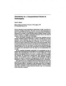
2013 for reviews). Common to all these studies is the underlying assumption that the brain generates actions from a limited number of modules (also called building blocks, primitives, muscle synergies, M modes, etc.) by reducing the number of parameters, or degrees of freedom, to be specified for the execution of a given motor task (Bernstein 1967). In particular for muscle activations, a large variety of movements performed during either rhythmic (e.g., locomotion) or discrete (e.g., whole body reaching) motor tasks have been shown to build upon modular structures (Tresch et al. 1999; d’Avella et al. 2003, 2006; d’Avella and Bizzi 2005; Ivanenko et al. 2004, 2005; Torres-Oviedo et al. 2006). However, the precise nature of these hypothetical modules has not been made clear yet, likely because many different models have been proposed and used successfully to infer candidate modules from electromyographic (EMG) data. In fact, each model makes specific assumptions, occasionally induced by the task under investigation, concerning the type and quantity of 1) the variables memorized to be reused in subsequent motor acts (i.e., the modules); and 2) the variables that have to be determined in every single motor act (i.e., the module activations). In a hierarchical view of motor control, these two different types of variables are assumed to be represented at different levels of the central nervous system (CNS), as illustrated in Fig. 1. Existing models of muscle modularity assume temporal (Fig. 1A), spatial (Fig. 1B) or integrated spatiotemporal modules (Fig. 1C). Here, we present a unified view by hypothesizing the concurrent existence of spatial and temporal modules (Fig. 1D); we refer to the proposed model as the space-by-time decomposition. In our framework, any single muscle pattern can be expressed as a double linear combination of spatial and temporal modules. Evidence for each type of module (spatial or temporal) has been separately reported in a large number of neurophysiological studies, which constitutes the basis of the unification property of the model: spatial modules correspond to the so-called synchronous, time-invariant or spatially fixed synergies; temporal modules correspond to the so-called muscle activation patterns, premotor drives, motor primitives, or temporally fixed synergies. Furthermore, the combination of several spatial and temporal modules can lead to time-varying synergies, i.e., genuine spatiotemporal muscle patterns, suggesting that the latter may originate from more primary build-

0022-3077/14 Copyright © 2014 the American Physiological Society

675

Innovative Methodology 676

A UNIFYING MODEL OF MUSCLE ACTIVATION MODULARITY

Fig. 1. Schematic representations of the logics of the different models used to extract modules in muscle space. A: temporal modularity model (Eq. 1). B: spatial modularity model (Eq. 2). C: spatiotemporal modularity model (Eq. 3). D: concurrent spatial and temporal modularity model (Eq. 4).

ing blocks in the CNS. Besides unifying, the key point of the space-by-time decomposition resides in the possibility to combine any of the temporal modules with any of the spatial ones, which leads to a low-dimensional but still flexible and taskrelevant representation of muscle patterns. In the following, we introduce the space-by-time decomposition model (see MATERIALS AND METHODS) and support the above assertions by means of a thorough analysis of its outcome when applied to real data (see RESULTS). The APPENDIX includes all the mathematical derivations related to the samplebased nonnegative trifactorization (sNM3F) algorithm that we designed to extract concurrent spatial and temporal modules from EMG datasets. Note that an open-source software implementation of the sNM3F algorithm is made available (see footnote).

and informed consent was obtained from all the participants, which was approved by the local ethical committee ASL-3 (“Azienda Sanitaria Locale,” local health unit), Genoa. The participants sat in front of a table and were instructed to perform center-out (forward, denoted by fwd) and out-center (backward, denoted by bwd) one-shot pointto-point movements between a central location (P0) and 4 peripheral locations (P1-P2-P3-P4) evenly spaced along a circle of radius 40 cm with either normal or fast speed. The targets to which the subjects reached were circles of radius 0.2 mm. In all recorded samples, the subjects touched the targets. Subjects were supporting the weight of their arm by themselves; no device was used to remove static gravitational effects. The upper trunk was not restrained, but analysis of the kinematics data showed that its movement during the investigated tasks was negligible. In total, the experimental protocol specified 4 targets ⫻ 2 directions ⫻ 2 speeds ⫽ 16 distinct motor tasks denoted by T1, T2, . . . ,T16. Each task was composed of 40 trials. Thus we had a number of muscles M ⫽ 9 and a number of samples S ⫽ 16 ⫻ 40 ⫽ 640, for each participant. The order with which the movements were performed was randomized. All subjects could perform easily the motor task. Data collection and preprocessing. Body kinematics was recorded by means of a Vicon (Oxford, UK) motion capture system. Six passive markers were placed on the finger tip, wrist (over the styloid process of the ulna), elbow (over the lateral epicondyle), right shoulder (on the lateral epicondyle of the humerus), back of the neck and left shoulder. The kinematics data were low-pass filtered (Butterworth filter, cut-off frequency of 20 Hz) and numerically differentiated to compute tangential velocity and acceleration. Movement onset and movement end were identified as the times in which the velocity profile superseded 5% of its maximum. Average movement duration varied across subjects from 370 to 560 ms for the fast speed movements and from 725 to 1092 ms for the normal speed movements. Electromyographic activity was recorded by means of an Aurion (Milan, Italy) wireless surface electrodes applied to lightly abrasive skin over the respective muscle belly. For each muscle, correct electrode placement was chosen so as to minimize crosstalk from adjacent muscles and tested by asking the subject to perform a number of movements and isometric contractions and observing the expected activation patterns (Ivanenko et al. 2004; d’Avella et al. 2006; Kendall et al. 1993). We recorded the activity of the following muscles: 1, finger extensors; 2, brachioradialis; 3, biceps brachii; 4, triceps medial; 5, triceps lateral; 6, anterior deltoid; 7, posterior deltoid; 8,

MATERIALS AND METHODS

Experimental Data Set Experimental design. The experimental dataset that we will use throughout this study is composed of the EMG activity recorded from nine upper body and arm muscles during execution of arm pointing movements in the horizontal plane (see Fig. 2 for an illustration). Six healthy right-handed participants participated voluntarily in the experiment. The experiment conformed to the declaration of Helsinki

Fig. 2. Illustration of the experimental procedure. The experiment consisted in 16 different point-to-point reaching movements in the horizontal plane(40 repetitions per motor task). EMG activity from nine muscles was recorded using surface electrodes and kinematic markers were placed on different body locations.

J Neurophysiol • doi:10.1152/jn.00245.2013 • www.jn.org

Innovative Methodology A UNIFYING MODEL OF MUSCLE ACTIVATION MODULARITY

pectoralis; and 9, latissimus dorsi. EMG signals were digitized, amplified (20-Hz high-pass and 450-Hz low-pass filters), and sampled at 1,000 Hz (synchronized with kinematic sampling). Subsequently, to extract the signal envelopes, the EMG signals were processed offline using a standard approach (d’Avella et al. 2006): the EMGs for each sample were digitally full-wave rectified, low-pass filtered (Butterworth filter; 20-Hz cutoff; zero-phase distortion), their duration was normalized to 1,000 time steps and then the signals were integrated over 20 time-step intervals yielding a final waveform of 50 time steps. For each one of the 6 subjects tested, we formed an EMG matrix of dimensions (50 time steps ⫻ 640 samples) ⫻ 9 muscles consisting of all the movement-related EMG activity (rectified and filtered) of the 9 muscles for all recorded samples. This matrix will serve as a test input for all decomposition algorithms presented below. Working Hypotheses and Terminology Before we proceed with the description of the newly proposed space-by-time decomposition model, we clarify the working hypotheses and specify the terminology used throughout the article. First, we review some basic principles of a theory of modular motor control that are important for a proper understanding of the proposed framework. Sample-independence in modular decompositions. We shall use the generic term sample to refer to a given trial of a given motor task for which one single motor pattern can be recorded using surface EMGs for example (in d’Avella and Tresch 2002, the term episode was used instead). Hence a sample is a single motor act generated by the brain to execute a given task. Usually, many samples are recorded during an experimental session to build a comprehensive dataset consisting of several tasks and several repetitions of the same task. According to the modular control theory, the CNS may generate motor behaviors in single samples by combining preexisting modules that are reused across behaviors. Therefore, when formalizing this theory mathematically, a fundamental constraint is to assume the sample-independence of these basis modules (loosely speaking, one could say that they are “invariant”). The need of this constraint rests on the hypothesis that modules are encoded and stored somewhere in the CNS (presumably in subcortical areas). In contrast, the activation coefficients, i.e., the neural drives that recruit the modules are sample-dependent and determine the motor output in every single sample. This dissociation between sample-independent and sample-dependent quantities allows making a clear distinction between variables under cortical control that are specified on a single-sample basis and variables that may be stored in subcortical areas and reused for subsequent actions. Such an interpretation is consistent with the idea of describing motor control based on a hierarchical organization (Scott 2004; Lockhart and Ting 2007; Tresch 2007). Spatial and temporal modularity. An important aspect of our work is the assumption of a concurrent existence of both temporal and spatial modularity. What we mean by temporal and spatial modularity is defined as follows. We call temporal modules the scalar functions of time that define the temporal structure of muscle pattern activations. This corresponds to what other authors previously referred to as muscle activation patterns, motor primitives, premotor drives/bursts, or temporally fixed muscle synergies (Ivanenko et al. 2005 2006; Chiovetto et al. 2010; Hart and Giszter 2004; Kargo and Giszter 2008; Hart and Giszter 2010; Safavynia and Ting 2012). We call spatial modules the multidimensional vectors defining the stereotypical patterns of ratios of activation across muscles at any given time. This corresponds to what other authors called time-invariant, synchronous, spatially fixed muscle synergies or muscle modes (Ting and Macpherson 2005; Ting and McKay 2007; Bizzi et al. 2008; Cheung et al. 2005, 2009; Overduin et al. 2008; Krishnamoorthy et al. 2003a,b). Functional requirements of modularity. When decomposing muscle activity into modules, it is important to bear in mind the functions that modularity should fulfill to be useful for motor control. First, modularity must simplify motor control. This means that each motor

677

pattern should be represented in a compact way and a small set of parameters should be sufficient to generate a genuine multidimensional and time-varying muscle pattern in each individual sample. Second, modularity must be adequate for achieving task goals. In other words, the activation of modules should be directly related to the motor task, and thus to the control of task-relevant variables. As an example, for an equilibrium maintenance task, muscle synergy activations have been shown to directly relate to the center of mass kinematics (Welch and Ting 2009). In sum, modularity should have a double functional role: the modular space should be lowdimensional to really simplify control and at the same time the associated modular structure should discriminate the tasks efficiently to support the view of a hierarchical organization of movement (i.e., from few task-relevant variables to complex coordinated muscle patterns). Thus, to assess models of muscle modularity, we need to evaluate them quantitatively in terms of the accomplishment of both functions (see Metrics to Critically Evaluate Modular Decompositions for additional explanations and RESULTS for a more detailed discussion). Taken together, the above considerations lay down the foundations of modular decomposition models and their critical assessment. In the following, we will first introduce the general scheme in which these ideas can be applied and then formalize them in terms of objective measures for the evaluation and comparison of different models. Also, by means of these concepts, we will address the functional and physiological interpretation of the extracted modules. Mathematical Models for Describing Modularity in Muscle Activity The most influential existing models for decomposing muscle activity into invariant modules can be clustered in three groups (see Fig. 1, A–C). Here, we will first describe all of them and then we will introduce the new model (see Fig. 1D). An empirical comparison of the properties of the three classes of model when applied to a simple well-studied motor task is given in Chiovetto et al. (2013). Depending on the model group and on the assumptions made about the underlying modular structure such as orthogonality, independence or nonnegativity, different algorithms can be used to extract the modules. Typical dimensionality reduction techniques include principal components analysis (PCA), independent component analysis (ICA), or nonnegative matrix factorization (NMF). Although each decomposition model can be implemented on EMG data using any of these algorithms, we restrict here to NMF-based decompositions that are physiologically more relevant for EMG signals, as nonnegative signals reflect well the “pull only” behavior of muscles (i.e., muscles cannot be activated “negatively”). Other dimensionality reduction algorithms have been discussed in the past (see Tresch et al. (2006) for a thorough comparison). Before presenting the decompositions, we denote the EMG dataset to be analyzed as M ⫽ [ms(t)]1ⱕsⱕS, where S is the total number of samples. The index s runs over all experimental samples, and thus spans all repetitions of all motor tasks. An element ms(t) of M is a multidimensional time series corresponding to the muscle signals collected at sample s. In practice, time is discretized so that we have T⫻M ms(t) 僆⺢⫹ , T being the number of time frames in that sample and M the number of muscles under consideration. Note that we use the notation wi(t) to emphasize that the signal is time-varying and not to denote its value at time t. The superscript s will characterize all sample-dependent quantities. Note that the duration of a sample is often normalized in muscle synergy studies, thus T is assumed to be constant across samples. Temporal decomposition model. In this model (referred to as temporal decomposition, illustrated in Fig. 1A), the muscle activity is represented as a linear combination of a set of one-dimensional time-varying patterns (temporal modules) that activate vectors of balance profiles across all muscles, as follows:



A UNIFYING MODEL OF MUSCLE ACTIVATION MODULARITY P

兺 wi(t)ais ⫹ residual i⫽1

m s(t) ⫽

(1)

T⫻1 where wi(t) 僆⺢⫹ is the i-th temporal module activated by the 1⫻M M-dimensional row vector asi 僆⺢⫹ and P is the total number of temporal modules (an input to the NMF algorithm). In this model, the sample-independent temporal modules wi(t) are waveforms over the entire time course of muscle activation and the parameters that have to be modified in each sample s are the vectors determining the muscle activation levels asi . As such, this model considers a primitive as a temporal pattern that will affect selectively different muscles. For example, this model has been used in Ivanenko et al. (2004). Spatial decomposition model. In this model (referred to as spatial decomposition, illustrated in Fig. 1B), a muscle pattern recorded during one sample s is represented as a linear combination of a set of time-invariant activation balance profiles across all muscles (spatial modules) activated by a time-varying activation coefficient, as follows:

m s(t) ⫽

N

asj (t)w j ⫹ residual 兺 j⫽1

(2)

1⫻M where wj 僆⺢⫹ is the row vector of muscle activation levels for the T⫻1 j-th spatial module; asj (t) 僆⺢⫹ is the time-varying coefficient for the j-th spatial modules at time t and N is the total number of spatial modules composing the dataset (an input to the NMF algorithm). Here, the sample-independent spatial modules are the time-invariant row vectors wj and the parameters that have to be specified in each sample s are the time-varying waveforms asj (t). As such, this model defines a synergy as a group of covarying muscles. This model has been used in Bizzi et al. (2008) and Tresch et al. (1999). Spatiotemporal decomposition model. Another type of model considered is the co-called time-varying synergies (d’Avella et al. 2003; d’Avella and Bizzi 2005; d’Avella et al. 2006, 2008, 2011), referred to as spatiotemporal decomposition and illustrated in Fig. 1C. In the framework of PCA, such models were already considered in Klein Breteler et al. (2007). These synergies are genuine spatiotemporal muscle patterns which do not make any explicit spatial and temporal separation. According to it, a single-sample muscle pattern is decomposed into time-varying muscle synergies combined as follows:

m s(t) ⫽

R

兺

k⫽1

askw k(t ⫺ ␴sk) ⫹ residual

(3)

T⫻M where wk(␶) 僆⺢⫹ is a vector representing the muscle activations for the k-th synergy at time ␶ after the synergy onset; ␴sk is the time of synergy onset and ask is a nonnegative scaling coefficient. This is a linear model providing a compact representation of the muscle activity during one sample s, because it has only two free parameters (one amplitude and one time coefficient) for each synergy. Note that the synergies wk are trial and task independent, whereas the parameters ␴sk and ask must be adjusted for each sample s. An NMF-like algorithm to extract these synergies has been developed in d’Avella et al. (2003) and, in the present study, we used a self-custom implementation of it. Space-by-time decomposition model: concurrent spatial and temporal modularity. In this work, we propose a new model (referred to as space-by-time decomposition, illustrated in Fig. 1D) to extract separately but concurrently spatial and temporal modules from recorded muscle patterns. The decomposition can be viewed as a generalization and unification of existing models and expresses any T⫻M muscle pattern ms(t) 僆⺢⫹ as the following double sum (T and M being the number of time frames and muscles, respectively):

m s(t) ⫽

P

N

兺兺 wi(t)aijsw j ⫹ residual, i⫽1 j⫽1

(4)

T⫻1 1⫻M where wi(t) 僆⺢⫹ and wj 僆⺢⫹ are the temporal and spatial s modules respectively, and aij 僆⺢⫹ is a scalar activation coefficient.

The parameters P and N correspond to the number of temporal and spatial modules respectively. To extract these concurrent spatial and temporal modules in practice, we developed a specific algorithm that seeks an approximate low-dimensional representation for all the input matrices called sample-based nonnegative matrix trifactorization (sNM3F, see APPENDIX). Briefly, the algorithm takes the parameters P and N as input and is designed (like the 3 previous ones) to iteratively minimize the total reconstruction error expressed as follows, where 㥋·㥋 denotes the Frobenius norm: E2 ⫽

P

N

wi(t)aijsw j 㛳2 . 兺s 㛳ms(t) ⫺ i⫽1 兺兺 j⫽1

(5)

The sNM3F algorithm thus performs a simultaneous extraction of concurrent spatial and temporal modules from rectified EMG data. We also considered some variants of this model. The most important variant attempts to capture variability in time, which may be inherent to the CNS’s modular control strategy, or which may simply be caused by the time-normalization procedure of the data or by any intrinsic fluctuation (e.g., sensorimotor noise). Specifically, we extended the trifactor decomposition to take into account time-shifted versions of temporal modules in the spirit of time-varying synergies d’Avella et al. (2003), as follows: m s(t) ⫽

P

N

兺兺 wi(t ⫺ ␴ijs)aijsw j ⫹ residual, i⫽1 j⫽1

(6)

where ␴sij is the time shift corresponding to sample s, temporal module i and spatial module j. Full details about the new model and the associated algorithms are deferred to the Appendix. Metrics to Critically Evaluate Modular Decompositions Variance accounted for. The variance accounted for (VAF) is the metric typically used in studies investigating modularity in muscle activations. It is defined as the residual reconstruction error defined in Eq. 5 normalized by the total variance of the dataset as follows: VAF ⫽ E2 ⁄

兺s 㛳ms(t) ⫺ m៮ 共t兲㛳2 ,

(7)

៮共t兲 is the mean muscle pattern across all samples. Note that where m another type of VAF is sometimes considered by replacing m ៮共t兲 by 0, but this latter version usually turns out to be less sensitive to changes in P, N, or R. The VAF measures the extent to which the original EMG patterns can be replicated using a limited number of temporal and spatial modules. In other words, it tells us whether the decomposition model used approximates well the dataset considered and can be used to validate or falsify the decomposition. However, the answer to this question can only be relative: the decomposition is valid only to a certain extent due to noisy fluctuations in biological data. Therefore, to assess the validity of a decomposition we consider a complementary metric that evaluates its discriminative power with respect to task variables (Delis et al. 2013b); this is the single-trial task decoding metric. Single-trial task decoding. The metric described here evaluates quantitatively if task goals can be decoded from the way modules are activated. Besides EMG data fitting, this is indeed a prerequisite for a theory of compositional motor control to be valid: the way modules are recruited by the CNS should determine the task executed as unequivocally as possible (see Delis et al. 2013b for a dedicated study about this metric). DECODING ANALYSIS. We used a linear discriminant algorithm in conjunction with a leaveone- out cross-validation procedure to predict the motor task executed in each sample using the single-sample parameters of each model. For the space-by-time decomposition, the decoding parameters are the N ⫻ P combination coefficients, i.e., the coefficients asij. For the spatial decomposition, we had to extract the decoding



parameters from the N time-varying activation coefficients. Among the endless possibilities of how to parametrize the time-course of the signal, we selected the time integral of the time-varying activation coefficient either over the entire movement period or binned in B equal subperiods (N ⫻ B parameters) because preliminary investigations (not shown) revealed that integral measures outperform the decoding performance obtained with other measures based on single points such as timing and amplitude of first or second activation peak and measures based on Principal Component Analysis of the activation time course. For the temporal decomposition, the single-sample parameters were the M spatiallyvarying muscle weighting coefficients which each of the P temporal modules is combined with (M ⫻ P parameters). We quantified decoding performance as the percentage of correct predictions and plotted the decoding results in the form of confusion matrices. The values on a given row h and column d of the confusion matrix C(d|h) represent the fraction of samples on which the executed task h was decoded to be task d. If decoding is perfect, the confusion matrix has entries equal to one along the diagonal and zero everywhere else. Performance at chance levels is reflected in a matrix in which each entry has equal probability 1/K, where K represents the number of repetitions of each task (K ⫽ 40 in our case). AUTOMATED SELECTION OF THE NUMBER OF MODULES BASED ON THE ABILITY TO DESCRIBE TASK-RELATED VARIABILITY. The core

idea of the model selection method resides in the fact that decoding performance should significantly improve only if inclusion of an additional module describes reliably some task-related EMG variations not described by other already included modules. When applied to spatial or spatiotemporal decompositions, this formalism was shown to be able to select reliably and robustly the smallest set of modules that describe all task-related information in the EMG data (Delis et al. 2013a,b). Extension of the method for the space-by-time decomposition is as follows. After evaluating decoding performance with (N, P) ⫽ (1,1), we consider adding either a spatial or a temporal dimension. i.e., increasing either N or P by one. We select the dimension that increases the most the decoding performance. Accordingly, we increase the number of modules step by step, until the increase of modules does not gain any further statistically significant increase of decoding performance. This procedure ensures the detection of modules that explain only the “task-relevant” variability and the exclusion of other sources of noise that produce “task-irrelevant” variability. RESULTS

Data Compression for Each Type of Decomposition Before applying the space-by-time decomposition model to physiological data, it is useful to consider the degree of dimensionality reduction it achieves and confront it with the other three models. A comparison of the number of parameters to be specified for a single sample in each decomposition is reported in Table 1, 1st row. Precisely, for a single sample s, the number of parameters to be specified to characterize a unique muscle pattern composed of TM values (T time frames ⫻ M muscles) is TN, PM, and 2R for the spatial, temporal and spatiotemporal decomposition respectively. For the space-bytime decomposition, the number of parameters is NP. If we assume that P ⬍⬍ T, N ⬍⬍ M and 2R ⬍⬍ TM then dimensionality reduction is effective in all the models. However, the extent to which dimensionality is reduced varies depending on the model considered. In fact, extracting only spatial modules results in controlling N continuous-time signals on a single sample basis. Extracting temporal modules leads to the control of P vectors specifying the weight of activation of all muscles.

679

Table 1. Dimensionality and storage capacity induced by each one of the four models under consideration Temporal Spatial Spatiotemporal Number of single-sample parameters Number of stored parameters

Space-byTime

PM

TN

R or 2R

NP or 2NP

TP

NM

TMR

TP ⫹ NM

The first row shows the number of parameters determined in each single sample of EMG activity for all models. The second row shows the number of parameters assumed to be invariant across samples and thus stored in order to be reused. T is the number of time frames, M is the number of muscles, while N, P, and R correspond to the number of modules to be extracted, chosen by the user. Models differ with respect to the extent to which they compress the original data and also their storage requirements.

The main issue with these two decompositions is that the dimensionality of the modular subspace depends on the time discretization (number of time frames T depends on the material used to collect data and on data processing; theoretically, it should even be infinite for continuous signals) or the number of muscles involved in the study (number of muscles M depends on the experimenter’s choice and on material/practical constraints). The spatiotemporal decomposition offered by the time-varying synergy model gives the best compression rate of the data since only a small finite number of scalar coefficients must be specified (R or 2R) and is independent of the number of time frames and muscles. The introduced space-by-time decomposition also exhibits a significant compression rate, similar to the time-varying synergies model (NP parameters, i.e., N spatial ⫻ P temporal modules). Importantly, this number is independent of the number of muscles and time frames under consideration. Models also differ substantially in terms of storage requirements (Table 1, 2nd row). The high compression rate of the spatiotemporal decomposition is balanced by its storage requirements: this model requires the storage of TMR parameters for R time-varying synergies. With T ⫽ 50, M ⫽ 9 and R ⫽ 6, this is a number of 2,700 parameters. From this point of view, the model is not very efficient since the number of parameters to be stored increases with the product TM. All other models require significantly less storage capacity. To give an order of comparison with the same data, the temporal decomposition requires the storage of TP ⫽ 300 values, the spatial decomposition requires the storage of NM ⫽ 54 values (both with 6 modules), and the space-by-time decomposition requires the storage of NM ⫹ TP ⫽ 27 ⫹ 150 ⫽ 177 values with N ⫽ 3 and P ⫽ 3 (a total of 6 modules as well). Therefore, for the same number of modules, depending on their nature, storage requirements may differ a lot, the rule of thumb being the complementarity between the number of parameters to set and the number of parameters to store. Interestingly, the space-by-time decomposition model implements an efficient trade-off: the number of parameters to set is independent of the number of time frames T and muscles M and the memory requirements depend only linearly on M and T. Note that this contrasts with the spatiotemporal decomposition which requires considerably more storage capacities when the number of time frames and the number of muscles is large.




Spatial and Temporal Structure Revealed by the Space-by-Time Decomposition We began the analysis by investigating what kind of spatial and temporal modules are found in experimental data recorded during the execution of arm pointing movements in different directions and with different speeds in the horizontal plane (see MATERIALS AND METHODS for details on the experimental protocol). For the sake of clarity, we first present the outcome of the decomposition for the dataset of a typical participant while the results for all six subjects follow in a subsequent section. We input the EMG data of the typical subject to the basic sNM3F algorithm to identify sample-independent spatial and temporal modules in muscle activity characterizing the set of motor tasks under consideration. Because the number of modules is unknown a priori, it appears as an input to the algorithm (as for any other dimensionality reduction method). Here, we performed extractions for N and P ranging from 1 to 9 (the number of muscles examined) to study the effect of these values on the estimated modules. Generally, we noticed that increasing the dimensionality in the temporal domain preserved the extracted spatial modules and vice-versa. Additionally, any new module was either added to the existing ones keeping them unchanged or arose from the splitting of one module into two. In other words, the main features of the modules identified in a set of (N, P) modules were preserved in a set with of (N ⫹ 1, P) or (N, P ⫹ 1) modules, supporting the robustness of the uncovered modular structure.

VAF and task decoding scores. We investigated the capability of the space-by-time decomposition model to reproduce the original muscle patterns and to describe the motor tasks under consideration in a low-dimensional space. The validity of a given modular decomposition can be critically evaluated using two metrics: 1) the percentage of the variability of the EMG dataset that is accounted for (VAF) by the decomposition and 2) the extent to which the single-sample coefficients of the decomposition distinguish each individual task from all others (task-decoding performance, see MATERIALS AND METHODS for explanations and Delis et al. 2013b). The first metric evaluates the goodness of reconstruction of the original EMG dataset while the second one quantifies the quality of the decomposition in terms of discrimination of task goals. We first studied the dependence of the VAF on the number of modules used and built the three-dimensional (3D) plot shown in Fig. 3A (VAF vs. N and P), which indicated that a small set of spatial and temporal modules (3 to 5) captured a large amount of the variance of the data. However, this threedimensional curve exhibited a steady increase with the number of modules without any clear saturation point and, therefore, selecting the best number of parameters revealed itself difficult on this basis. Then, we used a single-sample decoding analysis to evaluate quantitatively how well the single-sample combination coefficients, i.e., the coefficients asij for i ⫽ 1. . . P, j ⫽ 1. . . N, discriminate between different tasks. We decoded individual samples based on the single-sample measure of these

Fig. 3. Dependence of the variance accounted for (VAF) and task decoding metrics on the number of spatial and temporal modules extracted by the space-by-time model. A: VAF graph for the basic space-by-time decomposition without time shifts. B: VAF graph for the decomposition with time shifts. C: decoding performance graph for the basic space-by-time decomposition. D: decoding scores for the space-by-time decomposition with time shifts. J Neurophysiol • doi:10.1152/jn.00245.2013 • www.jn.org


parameters varying N and P and evaluated the decoding performance as the percentage of correctly decoded samples (see MATERIALS AND METHODS for details). On the resulting percent correct vs. N vs. P curve (Fig. 3C), we extended the automated method described in Delis et al. (2013b) to the 3D case for selecting the smallest set of modules that describe all taskdiscriminating information carried by the combinators. In brief, the method quantifies the decoding power afforded by the decomposition starting from (N, P) ⫽ (1, 1) and evaluates the significance of the decoding performance gain obtained when progressively adding modules. The method stops when inclusion of new modules does not add significantly to the decoding power of the decomposition. In this way, the selected set of modules is such that it explains all task-discriminating variability in the dataset. When applied to our dataset, the “path” followed by our method is represented by the arrows on the percent correct curve. At first, adding spatial modules contributes more to the task discrimination power of the model until N ⫽ 4. Then, our method indicates including two more temporal modules and stops at P ⫽ 3. Interestingly, the decoding graph exhibits a clear plateau, which helps to determine the smallest number of modules for our dataset. Hence, this analysis reveals that 4 spatial and 3 temporal modules correspond to the best decomposition in terms of the information about task-to-task differences. For N ⫽ 4 and P ⫽ 3, the VAF is 68% and the corresponding decoding performance is 80%. The modules identified by our algorithm are shown in Fig. 4A. The temporal structure of the dataset consists in three independently controlled activation bursts. This finding is compatible with the three independent phases of muscle activation in goal-directed movement execution, which has been documented in single-joint as well as multi-joint movements (Chiovetto et al. 2010; Berardelli et al. 1996). The spatial modules

681

reveal muscle groupings with a straightforward anatomical and functional interpretation (Fig. 4A, bottom). More specifically, the following four muscle groups are identified: elbow flexors, elbow extensors, shoulder flexors and shoulder extensors. Task-dependence of the spatial and temporal modules. To gain more insights into the functional role of the extracted modules for task performance, we examined how the activation parameters of the space-by-time decomposition are modulated by the task executed. To detect task-to-task differences in module activations, we computed the average of each entry coefficient asij at fixed task. For the selected set of modules, the number of coefficients asij per sample to be set is 4 ⫻ 3 ⫽ 12. In Fig. 5, we show in polar plots the dependence of these parameters on direction and speed. Speed modulation is apparent as the activation levels are much higher in motor tasks performed with fast speed compared with the ones performed with normal speed (black vs. grey curves). This result holds for movements to all directions and is compatible with previous experimental evidence (d’Avella et al. 2008). Then, we investigated the relationship between module activations and movement direction. In Fig. 5, columns of plots show the activation levels of different spatial modules combined with the same temporal module for all tasks. Thus, vertical observation reveals the functionality of different muscle groups at fixed temporal recruitment. For example, the first two spatial modules (elbow flexors and elbow extensors) are activated for opposite cardinal directions at all three movement phases. The same is true for the last two spatial modules (shoulder flexors and shoulder extensors). This observation validates the fact that the respective muscle groups constitute agonist-antagonist pairs for this set of motor tasks. Also, in the last phase of motion (corresponding to the activation of the third temporal module) the directional tuning of the activation

Fig. 4. Comparison of the modules identified by the space-by-time decomposition, with the ones extracted using alternative decompositions. A: 3 temporal (top) and 4 spatial (bottom) modules identified in the EMG data of the typical subject by the space-by-time decomposition. B: 3 temporal modules (top) extracted by the temporal decomposition and the four spatial modules (bottom) extracted from the spatial decomposition. C: temporal and spatial modules extracted by decomposing the 6 time-varying synergies, which are identified from the spatiotemporal decomposition, into spatial and temporal modules using the space-by-time decomposition. R values demonstrate the high similarity of the modules in B and C with the ones in A. J Neurophysiol • doi:10.1152/jn.00245.2013 • www.jn.org



Fig. 5. Polar plots of the directional and speed tuning of the activation coefficients that combine the 3 temporal and the 4 spatial modules to generate full EMG activation patterns. The 16 tasks (T1, . . . ,T6) specified by our experimental protocol involve movements of equal amplitude to 8 different directions (illustrated as points in the circumference of a circle) and with 2 different speeds: fast (depicted in black) and normal (in grey). Columns of the figure array correspond to activations of temporal modules, whereas rows correspond to activations of spatial modules.

coefficients is less apparent than for the first two phases. A possible interpretation for this is that many muscles are simultaneously activated in the last phase of motion to stabilize the arm over the final target. Such high muscle cocontraction has been shown to hold for different tasks involving fast point-topoint movements (e.g., Gribble et al. 2003). Similarly, horizontal observation shows the activation coefficients of different temporal modules combined with the same spatial module for all tasks. For instance, performance of motor tasks T5/T13 (fast out-center pointing starting from the left) requires an early strong activation of the posterior deltoid/ latissimus dorsi group (shoulder extensors) followed by an activation of the brachioradialis/biceps group (elbow flexors) and a final moderate coactivation of the triceps and finger extensors group (elbow extensors) and anterior deltoid/pectoralis group (shoulder flexors) which serves for decelerating the motion and stabilizing over the endpoint. Compatibility of the Modules with Other Models: Unifying Aspect of the Space-by- Time Decomposition In the following, we aimed at investigating the relation of the space-by-time decomposition with all the other decompositions. For this purpose, we applied the three other decompo-

sitions to the same EMG dataset of the typical subject. The subsequent qualitative analysis demonstrates the compatibility of the space-by-time decomposition with all existing ones and points out its unifying aspect. In all cases, to quantify the similarity between two extracted modules, we computed their correlation coefficient (R). The average correlation coefficient (R៮) across modules was used as a global index of similarity between two synergy decompositions. The temporal decomposition (Eq. 1) yielded temporal modules that were almost identical to the ones extracted by the space-by-time decomposition (R៮ ⫽ 1). In addition, the spatial modules identified by the spatial decomposition (Eq. 2) exhibited a very high similarity (R៮ ⫽ 0.96) with the spatial modules extracted by the space-by-time decomposition. This finding underlines that the new model subsumes the two existing ones and succeeds in determining the low-dimensional structure that is present both in the spatial and temporal domains. Then, we used the timevarying synergy model (Eq. 3) to identify spatiotemporal modules and investigate whether the extracted modules could be further separated into independent spatial and temporal ones. The idea is that these spatiotemporal patterns could possibly originate from concurrent spatial and temporal modules. To perform this, we fed the six spatiotemporal



modules extracted for this dataset (the number of time-varying synergies was determined by the decoding-based method) into the space-by-time decomposition algorithm (including time shifts) to uncover the underlying spatial and temporal structure. The result is depicted in Fig. 4C. Interestingly, both the temporal and the spatial modules extracted from this procedure are highly similar to the ones found by our algorithm (R៮ ⫽ 0.96 for the temporal modules and R៮ ⫽ 0.85 for the spatial modules). Thus, each time-varying synergy may actually be built from the spatial and temporal modules identified by our algorithm, suggesting that the underlying structure of the spatiotemporal modules may also rely on separate modularity in space and time, as assumed by the space-by-time decomposition model. This finding may suggest that the space-by-time model provides more primal building blocks than the spatiotemporal one. Actually, it can be shown that grouping spatial and temporal modules can lead to a set of time-varying synergies and, reversely, a dataset generated from time-varying synergies can always be decomposed according to the spaceby-time model. For both proofs we refer the reader to the Appendix. Note that to compare the temporal modules identified by the sNM3F algorithm with those extracted from the time-varying synergy model, we computed the cross-correlation over all possible time delays (because time-varying synergies can be shifted in time for each single sample) and found the highest similarity for a time delay ␴ ⫽ 11 (i.e., ⬃200 ms for movements of 1 s). This motivates testing the impact of incorporating time shifting also in the temporal modules of the spaceby-time decomposition. To examine this, we decomposed the same dataset using the space-by-time model with time delays (Eq. 6) and computed VAF and decoding performance of the resulting representations (Fig. 3, B–D). In these extractions, the delays were restricted to be nonnegative but similar results were obtained when allowing negatives delays as well (results not shown). A free parameter in the new algorithm is the maximum delay allowed during extraction. We tested two different values of the maximum delay: 1) half the normalized movement duration. and 2) one fifth of the normalized movement duration. Although the VAF metric reached higher levels for the same number of modules ([77% (1) or 74% (2) vs. 68% for (N, P) ⫽ (4, 3)], the corresponding decoding performance was lower than for the standard decomposition [66% (1) or 72% (2) vs. 80% for (N, P) ⫽ (4, 3)]. Thus, introducing the time-delays in the decomposition led to a better fitting of the original muscle patterns but reduced the ability of the model to describe unequivocally the different tasks. Also, the maximum delay parameter trades-off decoding performance for VAF: allowing longer delays increases the VAF but decreases the decoding performance. The reason for this decrease in the decoding performance when using the model with time shifts is twofold. First, the modules (especially the temporal ones) are modified by the inclusion of delays. In fact, the role of delays and combination coefficients may be interchangeable in some cases (a large time shift of a temporal module with an early burst can be equivalent to a non-shifted activation of a temporal module with a late burst).Thus, when we tried to decode the tasks using only the activation coefficients of the time-shifted version of sNM3F, we found significantly lower decoding performance compared with the basic sNM3F [66% (1) or 72% (2) vs. 80% for (N, P) ⫽ (4, 3)]. This result implies that the

683

simultaneous extraction of activation coefficients and time shifts has a slightly detrimental effect on the decoding power of the activation coefficients. Second, adding the time shifts to the set of decoding parameters did not increase the decoding performance of the model (it remained unchanged). A possible interpretation for this could be that the time shifts are useful to account for the different movement durations (which were normalized during data preprocessing). To address this, we also tested the impact of time shifts when using data from movements of similar duration (performed with fast speed only) and found similar results (not shown). It is also conceivable that, given that the temporal modules were active over the whole movement duration, the relatively poor performance of the time-shifted algorithm could be due to a truncation of the components associated with time shifts. To investigate this issue, we performed an additional analysis extracting temporal modules with durations equal to a fraction of the total normalized movement duration. We found that in such case the VAF was lower than the one we obtained when the module duration was equal to the entire movement duration (likely because more short modules may be required to get a large VAF), and the decoding performance with short modules never exceeded the one found with full-length modules (results not shown). For example, when using (N, P) ⫽ (4, 3), and temporal modules activated half the whole movement duration, we obtained for VAF and percent correct decoding values of 72.5 and 65% respectively, against the values of 77 and 66% obtained for module length equal to whole duration. Thus, using shorter modules did not seem to provide a task information gain from the data, and we concluded that this analysis does not support the view that truncation effects did play a major role in the relatively low performance of the time shifted algorithm. In sum, our results suggest that, for our data at least, time shifts do not relate strongly to task goals. Therefore, the time shifts mainly described task-irrelevant variability of the EMG data. It is nevertheless possible that, for another type of dataset, task performance will be more strongly encoded in the time shifts. Comparison of VAF and Decoding Across Models So far, we have shown that the space-by-time decomposition provides a parsimonious representation of muscle activation patterns that encompasses all currently considered models. Here, we compare quantitatively its performance to other decompositions using two objective and complementary metrics assessing the degree of validity of a given modular decomposition (i.e., VAF and task decoding). We recall that high VAF validates the decomposition for reconstructing accurately the original EMG data, whereas low VAF indicates a poor approximation on the associated linear subspace. In other words, this metric estimates the degree of dimensionality reduction achieved by the decomposition. On the other hand, high decoding performance lends credit to the model for mapping reliably the single-sample recruitment of modules onto task performance, while low decoding scores cast doubt on the usability of the decomposition for controlling movements. Simply put, this metric evaluates the extent to which a modular decomposition can describe effectively differences across motor tasks. In Fig. 6, we summarize the VAF and decoding results obtained when applying all the type of decompositions to the




Fig. 6. Summary and comparison of VAF (left) and decoding performance (right) scores obtained when applying all four decompositions to the EMG dataset of the typical subject. For the space-by-time model, the dependence of VAF (left) and decoding performance values (right) on the number of spatial and temporal modules are represented as matrices whose columns correspond to the contribution of temporal modules and rows correspond to the contribution of spatial modules. For the other 3 models, the dependence of VAF and decoding performance on the number of modules is represented as a vector whose entries are the numbers of modules considered. In the case of spatial modules, we also computed the decoding performance of the decomposition by binning the time-varying activation coefficients of the model and using as decoding parameters the time-integrals of the activations for each bin. Evaluating the decoding performance when varying the number of bins results in a matrix whose rows are the numbers of spatial modules and columns are the numbers of bins (right).

EMG data recorded from the typical subject. Note that when the number of spatial modules is equal to the number of muscles M, the output of our decomposition is equivalent to the results obtained from the temporal decomposition model. Similarly, when the number of temporal modules reaches the number of time points T, our decomposition is equivalent to the spatial decomposition model. We first compare the VAF across models. As already said, the VAF of our model (Eq. 4, 68% for N ⫽ 4 and P ⫽ 3) exhibited a smooth increase with the number of spatial and temporal modules extracted and reached asymptotically the VAF of the spatial decomposition model for high number of temporal modules (82% with N ⫽ 4 spatial modules) and the VAF of the temporal decomposition model for high number of spatial modules (73% with P ⫽ 3 temporal modules). Regarding the spatiotemporal decomposition model, we examined the VAF when neglecting the time shifts or not. In general, this decomposition reached higher values of VAF compared with the space-by-time decomposition with the same number of parameters per sample, meaning that with equal model complexity it approximated better the recorded EMG dataset. More precisely, with 6 time-varying synergies the VAF was 71% when ignoring time shifts whereas it was 80% when including time shifts (i.e., with 6 ⫻ 2 ⫽ 12 single-sample parameters). Considering the number of modules instead of the number of parameters per sample, the difference was however, smaller (68% with 7 modules in our case vs. 72% with 6 modules for the time-varying synergies). What remains to be tested is whether this higher reconstruction accuracy translates into a more reliable task discrimination on a single-sample basis. Decoding was significantly higher than chance level (1/16 ⫽ 6.25%) for all the models. As already said, the decoding performance of the space-by-time model saturated at the value of 80% at (N, P) ⫽ (4, 3). Increasing the number of spatial modules, we found that the discrimination power of the model approached asymptotically the corresponding performance found for the temporal decomposition (85% with N ⫽ 4 spatial modules). Then, to compare

with the decoding performance of the spatial decomposition, we restricted the number of decoding parameters of this model by binning the time course of the synergy activation coefficient asj (t) into B ⫽ 1 . . . 9 bins (see MATERIALS AND METHODS for details). This binning process corresponds to a dimensionality reduction in the time domain and yields a small number of parameters describing the data, which is in line with the idea of the space-by-time decomposition. In this case, binning also serves to avoid the “curse of dimensionality” that may arise when attempting to decode in very high-dimensional spaces. Indeed, the decoding power obtained by this process resembles very closely the one of the space-by-time model. This result reveals that the space-by-time decomposition had equal taskidentification power with the spatial decomposition when considering average muscle activations over shorter movement phases rather than the entire time-course of muscle activity. More importantly, the decoding performance of the spatial decomposition reached its maximum for a small number of bins (⬃3) and did not increase further. These three temporal bins and the corresponding decoding performance (78% with N ⫽ 4 spatial modules) resemble the three temporal modules identified by our algorithm that give similar decoding performance (80%). Thus, despite the potentially high number of free parameters describing the activation time course of spatial modules, the task being performed could be identified by reducing the dimensionality in the temporal domain to the three movement phases determined by the spaceby- time decomposition. Altogether, the above findings support that, besides its unifying aspect, the space-by-time decomposition model provides a good trade-off between low-dimensionality and taskrelevance. Moreover, the space-by-time decomposition afforded a significantly higher decoding performance than the spatiotemporal modules with equal complexity (80 vs. 70% with 12 parameters). In other words, the task-related differences in EMG signals were encoded more reliably by the single-sample parameters of the space-by-time decomposition than with those of the spatiotemporal decomposition. A possible explanation



resides in the structure of the space-by-time model, i.e., the dissociation between space and time. This translates into a double summation (Eq. 4), which indicates a combined activation of every temporal module with each one of the spatial ones, which is not the case when considering a monolithic spatiotemporal module. Hence, flexible task-dependent combination of the spatial and temporal modules may allow a better characterization of a wider variety of motor tasks. To further assess these differences on a task-by-task basis, we illustrated graphically the decoding results for these two models in the form of confusion matrices (Fig. 7). Each entry Ci,j of the confusion matrix represents the percentage of instances a motor task i is decoded by the decoding algorithm as j (see MATERIALS AND METHODS for details). For both models, confusions occurred primarily for neighboring motor tasks and were more pronounced in the case of backward movements (T5-T8 and T13-T16). The main difference between forward and backward tasks is that the former had the same starting point, while the latter had the same endpoint. Therefore, this finding may suggest that the endpoint is a movement feature encoded more reliably in the muscle activation patterns than the starting point. Additionally, tasks performed with normal speed (T9T16) are mislabeled more often than the fast speed ones. As speed correlates strongly with the level of muscle activation and also the time separation of movement phases, it appears that in lower speeds there were smaller differences in the activation coefficients from task to task which led to more confusions. Robustness of the Findings Across Subjects Besides the degree of plausibility of the space-by-time model that was quantified above, another critical aspect of the quality of the model concerns its consistence and generalization power. In this respect, it is important to test the robustness of the extracted modules across subjects. To investigate this, we applied the sNM3F algorithm to the EMG data recorded from the other 5 subjects to extract 3 temporal and 4 spatial modules and examined their pairwise similarity using as measure the average correlation coefficient. All extracted modules were highly similar across subjects. In Fig. 8, A–C, we present

685

the temporal and spatial modules obtained by averaging the extracted modules across subjects (we also show standard errors across subjects). Both of them are similar in shape and composition to the ones identified from the typical subject’s data: the temporal modules represent the three movement phases and the spatial ones correspond to functional muscle groupings. Therefore, for this set of tasks, the space-by-time model provides a generic, robust and unifying representation of muscle modularity in both the time and space domain. Furthermore, we examined the compatibility of the modules extracted by the space-by-time model with respect to all other models across all subjects. We found a high degree of similarity for all subjects when comparing the outputs of the spatial, temporal and space-by-time models (R៮ ⫽ 0.98 ⫾ 0.04 for the temporal modules and R៮ ⫽ 0.98 ⫾ 0.01 for the spatial modules). Also, the time-varying synergies (spatiotemporal model) could always be decomposed into separate spatial and temporal modules that were very similar to those extracted by the space-by-time model (R៮ ⫽ 0.93 ⫾ 0.07 for the temporal modules and R៮ ⫽ 0.94 ⫾ 0.05 for the spatial modules). This result verifies that the space-by-time model unified robustly all other models. A final assessment of the functionality of separate spatial and temporal modules relative to a genuine spatiotemporal representation consists in comparing the decoding and VAF scores of the space-by-time and spatiotemporal models when applied to the datasets recorded from all subjects. To perform a fair comparison, we used representations with the same number of free parameters: 6 spatiotemporal modules (6 ⫻ 2 ⫽ 12 single-sample parameters) vs. 3 temporal and 4 spatial modules (4 ⫻ 3 ⫽ 12 single-sample parameters). Results at the population level verify the findings of the analysis on the dataset of the typical subject (subject 5) showing a consistent and significant (paired t-test, P ⬍ 0.005) superiority of the space-by-time model in terms of task decoding ability (68.5 ⫾ 3.6 vs. 61.5% ⫾ 3.1%; Fig. 8B) whereas VAF is consistently and significantly (paired t-test, P ⬍ 0.01) higher for the spatiotemporal model (67.8 ⫾ 1.7 vs. 80.5 ⫾ 2.0%; Fig. 8D). A possible reason for this difference could be the presence of time shifts in the spatiotemporal model, which allows account-

Fig. 7. Confusion matrices illustrating the decoding performance of the space-by-time and the spatiotemporal decomposition on a task-by-task basis. Rows of the confusion matrix represent the actual motor tasks performed, while columns represent the decoded tasks. J Neurophysiol • doi:10.1152/jn.00245.2013 • www.jn.org



Fig. 8. Robustness of the extracted spatial and temporal modules across all subjects tested and comparison of the space-by-time decomposition with the spatiotemporal decomposition for all subjects. A: average of temporal modules across subjects. Shaded areas indicate standard errors. B: decoding performance of the space-by-time decomposition and the spatiotemporal decomposition with and without time delays. C: histograms of spatial modules across subjects. We report average values with the error bars indicating standard errors. D: VAF of the space-by-time decomposition and the spatiotemporal decomposition with and without time-delays. Subject 5 is the reference subject we used throughout the RESULTS.

ing for a larger part of the temporal variability that is present in the EMG signals. To address this, we also tested the space-by-time decomposition algorithm with time shifts (Eq. 6) and the spatiotemporal decomposition without time shifts.We note that these investigations aim to test the impact of the inclusion of time shifts on the VAF and decoding scores for either model. However, they do not allow a direct comparison of the two decompositions, because models with significantly different number of parameters are considered here. As expected, including time shifts increased significantly (paired t-test, P ⬍ 0.05) the VAF of the space-by-time decomposition (67.8 ⫾ 1.7 vs. 78.7 ⫾ 2.7%; Fig. 8D) but not the decoding performance (68.5 ⫾ 3.6 vs. 64.2 ⫾ 2.6%, Fig. 8B). The high impact of temporal delays in the VAF and not the decoding performance was also confirmed by the results we obtained when removing the delays from the spatiotemporal decomposition: on the one hand, the VAF of the spatiotemporal decomposition without delays was significantly smaller (paired t-test, P ⬍ 0.005) than when including delays (68 ⫾ 3.5 vs. 80.5 ⫾ 2.0%; Fig. 8D). On the other hand, the decoding performance did not change when removing delays (59.8 ⫾ 9.7 vs. 61.5 ⫾ 3.1%; Fig. 8B) . Thus, overall these results indicated that the introduction of time shifts always allowed for explaining a larger part of the variance of the dataset that was not, or at best was partly, related to differences across tasks. When comparing spatiotemporal and space-by-time models, we observed an interesting tradeoff: on the one hand, the spatiotemporal model without time shifts approximated the EMG data more parsimoniously in terms of single-sample parameters (only 6 scaling coefficients), while on the other hand, the space-by-time model was superior in characterizing differences across tasks (higher task discrimination power).

DISCUSSION

In this article, we proposed a space-by-time decomposition of muscle activations that models the simultaneous presence of separate stereotyped spatial and temporal modules. For this purpose, we developed a new algorithm that automatically extracts these putative modules from EMG data. We discuss below the pros and cons of the space-by-time model with respect to the VAF and task decoding metrics and we describe some possible applications of the model. Differential Contributions to Task-Related Variability and Quality of Reconstruction of Temporal and Spatial Modules Our results suggest that the space-by-time model is flexible and general enough to incorporate in a single framework the crucial features of existing temporal, spatial and spatiotemporal models. We found that the spatial and temporal modules obtained from the space-by-time model were very similar to those extracted from prior models. Moreover, the combination of these modules could be used to build the spatiotemporal modules identified by the time-varying synergy model, confirming that the spatial and temporal modules together constitute primary building blocks of genuine asynchronous muscle patterns. In the following, we discuss the ability of the different models to describe a variety of muscle patterns and motor tasks. Models differ greatly in terms of the number of parameters to specify on a single sample and to store within the CNS. Some models require more storage resources (the spatiotemporal model followed by the space-by-time model) while other simplify motor control less efficiently because complex signals remain to be determined in individual samples to fulfill task goals (the spatial and the temporal model). From the hierarchical control point of view, representing the muscle patterns



for a variety of motor tasks in a compact way is desired. However, this compression can be detrimental to the reconstruction error (VAF) and the discriminability of motor tasks (task decoding). These two metrics are complementary and capture different aspects of a given modular decomposition. The first aspect is dimensionality reduction: can we generate complex and adequate muscle patterns from a low-dimensional input space? The second aspect is task identifiability: can we capture all the salient task-to-task muscle activation differences even using a very low-dimensional EMG representation? Ideally, the VAF should be near 100% to support the existence of a linear low-dimensional structure in the EMG data. However, because surface EMG data are corrupted by various sources of noise, it is relatively hard to establish an absolute threshold for the VAF (even though standard values such as 90% have been employed in the literature). Besides neural noise, VAF values are also known to depend on the quality of data recordings (skin conductance, cross-talk etc.) and on data preprocessing (sampling, filtering etc.). In our analysis, because temporal and spatial models do not perform a large reduction of dimensionality of the data, a VAF ⬃90% could be obtained with 6 spatial or 9 temporal modules. The higher number of temporal modules suggests that compressing the dataset in the time domain affects the VAF more than compressing in space. At the same time, it is interesting to note that with 6 timevarying synergies (spatiotemporal model) a VAF ⬃80% could be obtained. Therefore, up to a relatively small loss of VAF (10%), using the spatiotemporal model muscle patterns can be represented much more compactly than with the temporal or spatial model. The criticality of such a 10% reduction of VAF is under debate. Comparing the task decoding scores of each decomposition could help to resolve this issue. In this respect, temporal modularity is more efficient in discriminating the motor tasks than spatial modularity (⬃85% with 3 temporal modules vs. 70% with 3 spatial modules). Put simply, the knowledge of which groups of muscles will be activated at different phases of the movement (temporal model) is informative about the task being performed but is less efficient in replicating the original muscle pattern. In contrast, the knowledge of the recruitment timing of different groups of muscles (spatial model) allows an accurate reconstruction of the original muscle patterns but carries less information regarding the task being performed. This duality between time and space is also apparent in the VAF and decoding curves. Using the space-bytime model, we observed a different behavior depending on whether time shifts were included in the model or not. Inclusion of time shifts contributed to an increase of VAF but not to the decoding power of the representation. From the algorithmic point of view, there are three potential reasons for this. The first (and perhaps most important) reason is that updating the time shifts relies on cross-correlation computations that do not guarantee the convergence of the NMF based algorithms. This can lead both sNM3F and time-varying synergy extraction to converge to suboptimal solutions more often. Second, and in particular for the sNM3F algorithm, the modules extracted by the timeshifted algorithm (especially the temporal ones) often differ from the ones extracted using the nonshifted algorithm. This makes it harder to interpret their functional role with respect to task performance. Third, as temporal modules manifest themselves as successive bursts of muscle activation, shifting one of

687

them in time for one trial will likely make it overlap with a subsequent one. From the functional point of view, it may be concluded that the role of time shifts is to refine the temporal resolution, which in turn allows building muscle patterns that replicate more accurately the original ones but does not seem to contribute to the encoding of task goals. Information about task goals is thus already present in global characteristic phases of the movement (e.g., acceleration or deceleration phase). Time shifts might rather account for sample-dependent taskirrelevant variability in movement repetitions (e.g., change in duration, joint trajectories etc., for instance induced by sensorimotor noise and/or feedback control mechanisms). A finer temporal resolution in muscle activity could also serve for encoding arm kinematics in continuous time. e.g., angular displacements or endpoint trajectory (not only the goal of the task as we assumed here). However, these considerations are beyond the scope of the present study and may require considering feedback control as well, while our focus here was on the formation of feedforward muscle patterns. In sum, in the arm pointing task examined here the spatiotemporal model offered the most parsimonious description of muscle activations (smallest number of modules leading to few single-sample parameters); the space-by-time model compensated the less efficient reduction of single-sample parameters with a smaller number of parameters to store and a more effective discrimination of different motor tasks. The difference in module dimensionality can be understood considering that the space-by-time model needs at least one spatial and one temporal module to generate a spatiotemporal module of synchronous muscle activations. To capture asynchronous patterns of activity like the spatiotemporal modules, multiple spatial and temporal modules are required. Thus, in the dataset we analyzed the space-by-time decomposition required a slightly larger number of muscle activation patterns to describe all tasks, which, however, led ultimately to a better decoding performance. Fully understanding the properties of the models considered here will require the analysis of more comprehensive EMG datasets. In our future work, we plan to apply the space-bytime decomposition to more complex motor behaviors with a wider range of motor tasks involving the activation of a larger number of muscles at different time scales. Possible Applications of the Proposed Model of Modularity Although simple temporal and spatial structures in muscle activities have been described separately in numerous studies, at least to our knowledge no previous study has attempted to extract both types of modules concurrently. Recently, Safavynia and Ting (2012) reported some concern about the existence of such a dual dimensionality reduction (in time and space), but analyzed the two problems separately. In the present study, we show that decomposition of muscle patterns in both time and space is actually efficient and provides a flexible scheme to create a variety of motor patterns for achieving various motor tasks. In the present study, we show that decomposition of muscle patterns in both time and space is actually efficient and provides a flexible scheme to create a variety of motor patterns for achieving various motor tasks. Other studies investigating the neural origins of modularity in muscle activations found evidence of the encoding of invariant




modules in the spinal cord and brainstem of frogs (Hart and Giszter 2010, 2004). However, focus was put only on temporal modularity because the authors assumed the existence of sample-independent premotor drives (i.e., temporal profiles of muscle activations). We believe that application of our new extraction algorithm to simultaneously recorded neural and muscle activities may allow identifying invariant temporal and spatial neural patterns and relating them explicitly to both primitives (i.e., temporal modules) and muscle synergies (i.e., spatial modules). Hence, modeling neural and EMG data with the space-by-time decomposition may help to uncover the direct link among the different levels of the hierarchical organization of motor control and lead to new insights in the quest of understanding the neural basis of modularity in the control of movements (Bizzi and Cheung 2013; Delis et al. 2010). Besides the fundamental knowledge that can be gained, a better understanding of how the brain controls movements is also important for applications such as neurorehabilitation (Safavynia et al. 2011; Cheung et al. 2012; Ethier et al. 2012; Jiang et al. 2010; Casadio et al. 2011; d’Avella et al. 2013) and neuroprosthetics (Ting et al. 2012; Morrow et al. 2009). The possibility of inferring motor goals from a small set of parameters and mapping this onto a complex coordinated motor pattern that will fulfill task goals is promising for humanmachine interfaces in general (Nazarpour et al. 2012; Radhakrishnan et al. 2008). Recently, it has been shown that the neural activity from the posterior parietal cortex can be used to decode not only variables related to the goals of movement but also 3D hand trajectories (Hauschild et al. 2012). Furthermore, electrical microstimulation of motor cortical areas was shown to activate spatial modules whose combination evoked specific hand movements (Overduin et al. 2012). Such a cortical representation of the recruitment of modules could be exploited to decode kinematic parameters of goal-directed movements. This is compatible with our findings since we showed that, besides task goal information, the modular structure also associates with the corresponding muscle patterns and therefore the corresponding arm trajectory. Thanks to this hierarchical control, very fast knowledge about the task goal and the feedforward motor pattern can be obtained from neural recordings (Quian Quiroga et al. 2006). Then, it is conceivable that this motor plan could be refined during online control via feedback control and cortico-spinal loops, and by the continuous recordings of neural signals during action execution (Hatsopoulos et al. 2004, 2007). In this sense, the development of generic mathematical models for modularity, such as the one presented here, should contribute to boosting both fundamental knowledge and applications of this line of research. APPENDIX

Sample-Based Nonnegative Matrix Trifactorization (sNM3F) In this subsection, we derive a dedicated algorithm for extracting simultaneously separate temporal and spatial modules from a given spatiotemporal datasets composed of multiple samples (trials and/or experimental conditions). The basic algorithm that we develop below is called “sample-based nonnegative matrix trifactorization” and we abbreviate it as sNM3F. Possible variants of the algorithm are presented thereafter. NMF (Lee and Seung 2001) is a powerful unsupervised learning technique that seeks to decompose a nonnegative matrix V as the

product of two nonnegative matrices GH as accurately as possible. The main feature of NMF is to provide a parts-based low-dimensional representation of the original data and has been used extensively in the context of muscle synergy extraction (Tresch et al. 2006). In this context, the data are bidimensional (with a space and a time dimension). Moreover, many samples are available as the result of repeating the same experimental condition or testing various conditions. The straightforward application of the standard NMF algorithm to such data sets typically yields the product of a sample-independent matrix and a sample-dependent matrix, whose functional meaning depends on whether different samples were concatenated in rows or columns of the input matrix V (see below). NM3F is an extension of NMF that can be used to decompose bi-dimensional data in both rows and columns separately and simultaneously (Ding et al. 2006), without making the a priori assumptions as to whether the dataset has a temporal or a spatial low-dimensional structure. Without particular constraint on the factors to be extracted, NM3F actually reduces to a classical NMF. However, when introducing constraints on the factors to be extracted, the outcome of NM3F generally differ. In our context, the constraint comes from the sampleindependence requirement for 2 factors of the decomposition. Even though NM3F algorithms exist (Ding et al. 2006), we had to develop a specific algorithm to handle our specific sample-independence constraint that naturally arises in the context of compositional motor control theory. This particular method is called sample-based NM3F (shortly sNM3F) and has the desired feature of decomposing the data into two sampleindependent matrices (called spatial and temporal modules) which are combined through one low-dimensional sampledependent matrix (activation coefficients, which are scalars here). The basic sNM3F algorithm is first described and useful extensions are then proposed. Its effectiveness will be illustrated for simulated data.

Description

of

the

basic

sNM3F

algorithm.

PROBLEM

Let M ⫽ (Ms)1ⱕsⱕS be a set of nonnegative matrices T⫻M , where T is the number of time steps whose elements belong to ⺢⫹ and M is the number of spatial dimensions (e.g., different EMG electrodes placed at various body locations) and the index s is used to indicate one sample. The goal is to find an approximate low-dimensional representation of M for the space-by-time model (Eq. 4). Formally, our goal is to factor each one of the elements of M as follows: FORMULATION.

˜ sW for all s 僆 [1, S] M s ⬇ WA

(8)

T⫻P ˜ 僆⺢⫹ is a matrix whose columns are the temporal modwhere W N⫻M ules, W 僆⺢⫹ is a matrix whose rows are the spatial modules and P⫻N As 僆⺢⫹ is the matrix containing the coefficients combining each one of the P temporal modules with each one of the N spatial ones. The above trifactorization (Eq. 8) can be rewritten more explicitly as the following double sum:

m s(t) ⫽

P

N

兺兺 wi(t)aijsw j ⫹ residual i⫽1 j⫽1

(9)

where ms(t) represents a time-sequence of signals for sample s, P, and N are the number of temporal and spatial components respectively, wi(t) and wj correspond to the columns of W˜ and the rows of W respectively, and (asij)1ⱕiⱕP,1ⱕjⱕN are the elements of the matrix As (which are also denoted by Asij below). Note that our specific con˜ and W. Therestraint is to seek for sample-independent matrices W fore, the goal is to find the set of matrices A ⫽ (As)1ⱕsⱕS together with the matrices W˜ and W that minimize the total reconstruction error: E2 ⫽ with


兺s Es2

(10)


˜ sW㛳2 ⫽ Es2 ⫽ 㛳M s ⫺ WA

˜ sW)u,v兴2 . 关 M su,v ⫺ (WA 兺 u,v

(11)

The product PN is the dimension of the linear space from which each element Ms of M can be represented and the dimensionality reduction will be effective if PN ⬍⬍ TM. ALGORITHM DERIVATION. By convention, we represent the set of matrices M ⫽ (Ms)1ⱕsⱕS as a matrix built from a vertical concatenation of all the samples, that is:

冢冣 M1

M⫽

M2 É

.

MS

Definition. The block transpose operation, denoted by the symbol “prime”, transforms a matrix M with vertical concatenation of the samples to M= with horizontal concatenation of the samples and vice-versa. Thus M= ⫽ (M1 M2 . . . MS) and 共M=兲= ⫽ M. The standard NMF decomposes any nonnegative matrix as follows: M s ⬇ G sH s . In our context of multiple samples (indexed by s), two types of decomposition can be obtained depending on how the samples are arranged (either vertical or horizontal concatenation). For a vertical concatenation of samples, the following decomposition can be obtained:

冢冣冢冣 M1

M⫽

M

G1

2

É

MS

⬇

G2 É

W ⫽ GW

(12)

GS

b) Compute H ⫽ AW c) Get H= (block transpose) ˜ =, d) Update W˜ to improve the approximation M= ⬇ WH ˜ i,j ← W ˜ i,j 共M=H兲i,j (WH=H) ˜ i.e.: W for i 僆关1, T兴 and j 僆 i,j 关1, P兴 ˜ update A as follows: 4) Given W and W, a) For all s 僆关1, S兴, update As to improve the approximation s s ˜ sW, i.e.: Ai,j ← Ai,j 共W˜ TM sWT兲i,j 共W˜ TAsW兲WT)i,j for M s ⬇ WA i 僆关1, P兴 and j 僆关1, N兴 5) If the decrease in E2 is below a given tolerance, stop. Otherwise go back to step 2. Proof of convergence. The proof of convergence follows from the ones of the 2-factor and 3-factor cases, which are available in Lee and Seung (2001) and Ding et al. (2006) respectively. In brief, we need to show that the total reconstruction error E2 is nonincreasing under the three multiplicative update rules (rules 2c, 3d, and 4a) of our algorithm. First, it is immediate that E2 is nonincreasing under the update rules 2c and 3d because they correspond to the standard update rules of a 2-factor NMF. The key point here is simply that the block transpose operation does not affect the error E2. In fact, the algorithm alternates between a right-side and a left-side update for input matrices M or M=, respectively. The proof that the first two multiplicative rules do not increase the reconstruction error is given in Theorem 1 in Lee and Seung (2001). Additionally, we need to show that the third update rule 4a does not increase the total reconstruction error E2. Theorem 8 in Ding et al. (2006) shows that the single-sample error Es2 is nonincreasing under the multiplicative rule 4a and, because the total error is just the sum of Es2 over all samples, also E2 is nonincreasing. This completes the proof of convergence of the algorithm.

Ⲑ

Ⲑ

Variants with orthogonality constraints and time shifts.

where W would be the sample-independent matrix. In this case, the NMF algorithm performs dimensionality reduction in the columns of the input matrix M=, which corresponds to the extraction of spatial modules only (see Eq. 2). On the other hand, for a horizontal concatenation, one gets: ˜ M= ⫽ 共M1 M2 · · · MS 兲 ⬇ W˜ 共H1 H2 · · · HS 兲 ⫽ WH=. (13) ˜ is the sample-independent matrix and the NMF In this case, W algorithm performs dimensionality reduction in the rows of the input matrix M=, which corresponds to the extraction of temporal modules only (see Eq. 1). The meaning of these two decompositions differs and, in the context of the modular control of movement, making such an a priori choice may undesired. This motivates the use of a trifactor decomposition that combines the two presented above. The core idea is to simultaneously and alternatively perform the two decompositions, i.e., to reduce dimensionality in both dimensions, by taking into account the sample-independence constraints. Keeping in mind that the free parameters P and N representing the number of sample-independent modules must be specified by the user, the steps of the sNM3F algorithm are as follows, based upon Lee and Seung (2001) and Ding et al. (2006).

Algorithm (sNM3F). ˜ A= ⫽ (A1 A2 . . . AS) and W 1) Initialize W, = ˜ update W as follows: 2) Given A and W, ˜ = a) Compute G= ⫽ WA b) Get G (block transpose) c) Update W to improve the approximation M ⬇ GW, i.e.: Wi,j 4 Wi,j (GTM)i,j (GTGW)i,j for i 僆关1, N兴 and j 僆关1, M兴 3) Given A= and W, update W˜ as follows: a) Get A (block transpose)

Ⲑ

689

Biorthogonality In many occasions, it is convenient to further impose ˜ IdP⫻P orthogonality constraints on the matrices W˜ and W, i.e., W˜ TW⫽ and WWT ⫽ IdN⫻N. Under this biorthogonality constraint, the NM3F can be seen as a generalization of clustering as explained in Ding et al. (2006). Imposing such constraints involves the use of Lagrange multipliers in the derivation of the algorithm. From Eqs. 27 and 28 in Ding et al. (2006), it is apparent that the two first update rules of the above algorithm have to be adapted. The last update rule is kept unchanged since no constraint (except nonnegativity) is applied to A. More precisely, the rule 2c rewrites: Wi,j ← Wi,j

(GTM)i,j (GTMWTW)i,j

for i 僆关1, N兴 and j 僆关1, M 兴

and the rule 3d rewrites: ˜ i,j ← W ˜ i,j W

(M=H)i,j ˜ W˜ TM=H)i,j (W

for i 僆 [1, T] and j 僆 [1, P]

TIME SHIFTS. In this subsection, we extend the trifactor decomposition to include time-shifted versions of temporal modules as follows:

m s(t) ⫽

P

N

兺兺 wi(t ⫺ ␴i,js)ai,jsw j ⫹ residual. i⫽1 j⫽1

(14)

The introduction of time shifts (␴si,j ⱖ 0), in the spirit of the timevarying synergies (d’Avella and Tresch 2002), makes the derivation of the decomposition algorithm slightly more involved. Note also that it breaks the proof of convergence and may affect the algorithm’s stability and convergence speed. Whenever a signal wi(t) is time shifted, the practical rule is to put zeros for all t ⬍ ␴si,j in the resulting T signal. Remember that after time discretization, wi(t) 僆⺢⫹ . Although we restrict to positive time shifts in this paper, extending the model to also deal with negative time shifts is straightforward with minor modifications.




Factorization with the time shifts (single sample). The time-shifting operation of a vector wi(t) corresponds to the multiplication with a T⫻T sub-diagonal matrix Dsi,j 僆⺢⫹ whose first nonzero element is at row s s ␴i,j ⫹ 1. Note that ␴i,j is basically an integer due to the time discretization. If negative time shifts were to be considered, the TPN⫻TPN transpose of Dsi,j could be used instead. Let Ds 僆⺢⫹ be the block diagonal matrix obtained by concatenating all the Dsi,j matrices along the diagonal (starting with all the indexes i ⫽ 1 . . . P for j ⫽ 1, and so on until j ⫽ N). It is now possible to write the decomposition with the time shifts for a given sample s as follows: M s ⬇ Wˆ sAˆ sW s ˜ ˜ 关P兴兲 ˜ 关1兴, . . . , DsP,1W ˜ 关P兴, . . . , D1,N W关1兴, . . . , DsP,NW where Wˆ s ⫽ 共Ds1,1W T⫻PN ˜ ˜ and: ,W关 j兴 denoting the j-th column of W, 僆⺢⫹

冢冣 As11 É

Aˆ s ⫽

AsP1

Ì

s A1N

Proof that the space-by-time decomposition subsumes the spatiotemporal decomposition. In this section, we aim to show that

PN⫻N 僆⺢⫹ .

É

AsPN

Update rule for A. After some simple calculations, we can show that the rule 4(a) for updating the matrices As for s 僆关1, S兴 has to be replaced by the following one: (Wˆ sTM sWT)(j⫺1)P⫹i,j s s Ai,j ← Ai,j for i 僆 [1, P], j 僆 [1, N] sT (Wˆ (Wˆ sAˆ sW)WT)(j⫺1)P⫹i,j Factorization with the time shifts (merging all samples). We can write the decomposition including all samples as a single trifactorization as follows: ˆ M ⫽ QAW TS⫻PNS where Q ⫽ diag 共Wˆ 1, . . . , Wˆ S兲僆⺢⫹ is a block diagonal matrix PNS⫻N is the vertical concatenation of all the matrices Aˆ s. and Aˆ 僆⺢⫹ ˜ Computing the gradient of the total reconstrucUpdate rule for W. ˜ i,j brings us to define the tion error E2 (Eq. 5) with respect to W TS⫻PNS 共ij兲 : following matrix ⌰ 僆⺢⫹

⌰(ij) ⫽ where ⌰n共ij兲 is block 共⌰n共ij兲,1, . . . , ⌰n共ij兲,S兲, with:

N

n 兺 ⌰(ij) n⫽1

diagonal

defined

as

⌰n共ij兲

⫽

diag

s ⌰(ij),s ⫽ matr(D[(n⫺1)TP⫹(j⫺1)T⫹i] ), n TPN T⫻PN to ⺢⫹ . in which matr denotes the matrization from ⺢⫹ After some calculations, it can be seen that the multiplicative update rule 3d has to be replaced by: ^

˜ ij ← W ˜ ij W

tr[MT⌰(ij)H] ^

^

tr[(QH)T⌰(ij)H]

peak), crosscorrelations were computed between the original data and the component wi(t)wj. The index j yielding the maximum crosscorrelation was picked up, as well as its corresponding time-lag ␴si,j, and the quantity wi(t ⫺ ␴si,j)asi,jwj was subtracted from the input matrix Ms. The process was repeated using the residual part of Ms until all the spatial components indexed by j had been picked up. After that, the procedure jumped to the next index i and the previous step was repeated, still using the residual part of Ms. Once all j, i, and s indices had been covered, the procedure stops.The second update rule was conceived with unsigned time shifts in mind. This consists in selecting at each iteration the space-by-time component (i.e., the pair wi(t), wj) with the highest cross-correlation. Our tests (not reported) did not reveal significant changes if one or the other update rule was used, Therefore, here we report results obtained using only the first update rule. An open question for future research is the investigation in convergence differences and algorithm performance for the two rules in other datasets. Update rule for W. This rule is analogous to the one given in 2(c) of the sNM3F algorithm.

for i 僆 [1, T] and j 僆 [1, P]

ˆ Note the similarity between this update rule and the where Hˆ ⫽ AW. one presented in d’Avella et al. (2003) (see their Equation 7). Update rule for the time shifts ␴si,j. The rule for updating the time shifts ␴i,j is a generalization of the best matching procedure presented in d’Avella and Tresch (2002). We propose two ways to do this. The first one was thought with nonnegative time shifts in mind, but could also be applied to unsigned time shifts. In such case„ the time-varying signals wi(t) were first ordered with respect to the time occurrence of their maximal value. Then, for each sample s and each temporal component wi(t) (going backwards from the signal with the latest

the proposed space-by-time decomposition subsumes the spatiotemporal decomposition. To do this, we first show that the combination of several spatial and temporal modules from the space-by-time decomposition yields time-varying synergies of the spatiotemporal decomposition. To prove this statement, let us define the Cartesian product K ⫽ I ⫻ J with I ⫽ (1, . . . ,N) and J ⫽ (1, . . . ,P). For a given 1 ⱕ R R ⱕ NP, let us choose some partition of K, i.e., K ⫽ 艛 k⫽1 Uk. We can now rewrite Eq. 4 as follows: m s(t) ⫽

R

兺兺 wi(t)aijsw j . k⫽1 (i,j)僆u k

If we further assume that the asi,j are identical within a given set Uk, we obtain: m s(t) ⫽

R

兺 askwk(t), k⫽1 兺

with ask ⫽ asi,j for (i, j) 僆 Uk and wk(t) ⫽ 共i,j兲僆Uk wi共t兲wj. Note that R can be chosen arbitrarily as well as the partition of K, which means that many different time-varying synergies can be obtained from Eq. 4. Interestingly, the R time-varying synergies are just linear combinations of the original spatial and temporal modules. Adding the case of temporal delays is straightforward and therefore, up to some reorganization in the double sum, it can be concluded that the spatiotemporal decomposition is a by-product of the space-by-time decomposition. Conversely, to complete the proof, we also show that a dataset generated from a given family of R time-varying synergies can be decomposed according to the space-by-time model. Obviously, the answer is affirmative and the proof is constructive: we define M spatial modules (w1, . . . ,wM) recruiting a single muscle at time [wi ⫽ (␦ij)j⫽1 . . . M, ␦ij denoting the Kronecker symbol]. We define RM temporal modules that equate the temporal activation of each muscle within each time-varying synergy, i.e., we define w11(t), . . . , w1M(t), . . . , wR1(t), . . . , wRM(t). Then it is possible to write each time-varying synergy as follows, for k ⫽ 1 . . . R: w k(t) ⫽

M

兺 wki(t)wi . i⫽1

Again, dealing with temporal delays is straightforward. Note that using afterwards these spatial and temporal modules allows generating more muscle patterns than what is allowed originally by the spatiotemporal modules. This reflects the greater flexibility offered by the combination of separate spatial and temporal modules. This construction however, involves the canonical basis of ⺢ M , which means that a spatial module only activates a given



691

ALTERNATIVE ALGORITHMS FOR EXTRACTING SPATIAL AND TEMPORAL MODULES.

Fig. 9. Comparison of two successive nonnegative matrix factorization (NMF) and the sample-based nonnegative matrix trifactorization (sNM3F) algorithm on a random simulated dataset. The two first bars show the root-mean-squared (RMS) residual for the 2 possible sequence of NMFs while the last bar is the rms residual for the sNM3F method. The small vertical lines indicate the standard deviation of the rms residual across all runs (n ⫽ 100).

muscle, and it also involves the use of a unique temporal waveform for each pair muscle/module (RM temporal modules needed). Nevertheless, this construction shows that any set of time-varying synergies can be theoretically rewritten in the form of Eq. 9. Overall, this paragraph demonstrates that the space-by-time decomposition subsumes the spatiotemporal decomposition and justifies the reason why it may be possible to find evidence for both types of decompositions in EMG data (see RESULTS).

The space-bytime decomposition (Eq. 4) can be implemented by means of other families of dimensionality reduction algorithms (such as PCA or ICA), as is the case for all decompositions of muscle activities presented here (temporal, spatial or spatiotemporal). Restricting the analysis to the case of nonnegative signals, a simple alternative algorithm performing two successive NMFs could be considered to identify sample-independent spatial and temporal modules. Indeed, by first finding out the spatial modules using the factorization in Eq. 12 (M ⬇ GW), one can subsequently apply another NMF to the block-transpose of the matrix G to obtain the temporal modules (this time from a factorization similar to the one in Eq. 13). This basic procedure allows to extract sample-independent spatial and temporal modules compatible with the decomposition written in Eq. 4. Similarly, one could also extract the temporal modules before the spatial modules. However, this method contrasts with the sNM3F algorithm which attempts to extract both temporal and spatial modules at once. Although a debate about alternative algorithms is out of the scope of the present study, a simple comparison between the two proposed algorithms (showing the greater robustness and performance of the sNM3F algorithm compared with a double NMF) is reported below.

Illustration of the Method with Simple Data Sets Comparison of algorithms: two successive NMFs vs. basic sNM3F. Here we used numerical data constructed from random

nonnegative matrices. We set M ⫽ 20, T ⫽ 20, S ⫽ 50, N ⫽ 10 and ˜ sW for s ⫽ 1 . . . S. We then P ⫽ 10 and built the matrices Ms ⫽ WA applied either two successive NMFs or the sNM3F algorithm to try to

Fig. 10. Application of sNM3F with time shifts to simulated muscle activations and robustness to noise. A: simulated dataset (9 muscles and 5 samples). B and C: 2 temporal and three spatial modules extracted. The r values represent correlation coefficients between the original and the reconstructed modules. J Neurophysiol • doi:10.1152/jn.00245.2013 • www.jn.org



discover the lowdimensionality of the data. The tolerance and the maximum number of iterations was the same for all algorithms. The NMF was based on the Matlab function nnmf using the multiplicative update rule option.1 Several runs (n ⫽ 100) were performed to test the robustness and performance of each extraction method. The results are presented in Fig. 9. It is visible that the sNM3F algorithm yields significantly lower root mean squared residual (兹E2⁄TMS, see Eq. 5) than the method involving two successive NMFs (t-test, P ⬍ 0.001). Moreover, the sNM3F algorithm appears to be more robust than the alternative algorithm (lower standard deviation across runs). Overall, this test shows that the sNM3F appears to be more efficient for the purpose of decomposing data following Eq. 4.

Simulated data with known spatial and temporal modules. To illustrate and test the effectiveness of the sNM3F algorithm, we generated a simple EMG dataset by combining a set of known spatial and temporal modules.The purpose of this simulation is to demonstrate that if a dataset indeed originates from the combination of separate temporal and spatial modules then the space-by-time decomposition implemented using the sNM3F algorithm can uncover the underlying structure. To this aim, we simulated the coordinated EMG activity of 9 muscles recorded during 100 samples. The EMG data were generated using two temporal modules and three spatial ones. The temporal modules were simulated as two Gaussian bursts with different centers, widths and amplitudes (Fig. 10B) and were timeshifted in each sample by a random delay varying for 0 to 10 time frames. Each one of the three spatial modules consisted of the activation of three muscles with random levels to indicate the existence of three distinct groups of covarying muscles (Fig. 10C). We simulated 100 samples of duration 50 time steps by combining each one of the simulated temporal modules with each one of the spatial modules with random sample-dependent combination coefficients (Fig. 10A). Thus, and importantly, each spatial and temporal module contributes independently to the generation of these data. We applied the sNM3F with time shifts (Eq. 6) to the resulting dataset as well as the three other NMF-based decomposition models. The sNM3F reconstructed both the spatial and temporal modules from which the data were generated with high accuracy (Fig. 10, B and C, see r values representing correlation coefficients between the original and the reconstructed modules). The variance of the dataset accounted for (VAF) by our decomposition was 99%. We repeated the extraction 10 times with random initializations of the matrices. In all cases, the algorithm converged accurately to the original modules. The possibility to accurately recover the correct modules is here related to the sparsity structure of the chosen modules whereas in general the decomposition may not be unique and, therefore, many equivalent sets of modules yielding the same reconstruction error can be obtained. Then we aimed at evaluating the robustness of the decomposition algorithm to noise. To test this, we added white Gaussian noise to the matrix of EMG activations varying the noise parameter n from 0.1 to 0.5. This parameter determines the level of noise as a fraction of the highest EMG activation. The algorithm recovered the original structure of the data accurately for all levels of noise (r៮ ⫽ 0.95 ⫾ 0.4 for the temporal modules and r៮ ⫽ 0.99 ⫾ 0.04 for the spatial modules). ACKNOWLEDGMENTS We are indebted to Enrico Chiovetto for valuable comments on the manuscript. GRANTS We acknowledge the financial support of the SI-CODE project of the Future and Emerging Technologies (FET) programme within the Seventh Framework 1 A Matlab (Mathworks, Natick, MA) code implementing the basic sNM3F algorithm as well as its variant with time shifts can be found at http:// hebergement.u-psud.fr/berret/software/sNM3F.zip.

Programme for Research of The European Commission, under FET-Open grant number: FP7–284553. DISCLOSURES No conflicts of interest, financial or otherwise, are declared by the author(s). REFERENCES Alessandro C, Delis I, Nori F, Panzeri S, Berret B. Muscle synergies in neuroscience and robotics: from input-space to task-space perspectives. Front Comput Neurosci 7: 43, 2013. Berardelli A, Hallett M, Rothwell JC, Agostino R, Manfredi M, Thompson PD, Marsden CD. Single-joint rapid arm movements in normal subjects and in patients with motor disorders. Brain 119: 661– 674, 1996. Bernstein N. The Coordination and Regulation of Movements. Oxford, UK: Pergamon, 1967. Bizzi E, Cheung VC, d’Avella A, Saltiel P, Tresch M. Combining modules for movement. Brain Res Rev 57: 125–33, 2008. Bizzi E, Cheung VCK. The neural origin of muscle synergies. Front Comput Neurosci 7: 51, 2013. Bizzi E, Mussa-Ivaldi FA, Giszter S. Computations underlying the execution of movement: a biological perspective. Science 253: 287–291, 1991. Casadio M, Pressman A, Acosta S, Danzinger Z, Fishbach A, Mussa-Ivaldi FA, Muir K, Tseng H, Chen D. Body machine interface: Remapping motor skills after spinal cord injury. In: IEEE Int Conf Rehabil Robot, 2011, p. 1– 6. Cheung VC, d’Avella A, Tresch MC, Bizzi E. Central and sensory contributions to the activation and organization of muscle synergies during natural motor behaviors. J Neurosci 25: 6419 –34, 2005. Cheung VC, Piron L, Agostini M, Silvoni S, Turolla A, Bizzi E. Stability of muscle synergies for voluntary actions after cortical stroke in humans. Proc Natl Acad Sci USA 106: 19563–19568, 2009. Cheung VCK, Turolla A, Agostini M, Silvoni S, Bennis C, Kasi P, Paganoni S, Bonato P, Bizzi E. Muscle synergy patterns as physiological markers of motor cortical damage. Proc Natl Acad Sci USA 109: 14652– 14656, 2012. Chiovetto E, Berret B, Delis I, Panzeri S, Pozzo T. Investigating reduction of dimensionality during single-joint elbow movements: a case study on muscle synergies. Front Comput Neurosci 7: 11, 2013. Chiovetto E, Berret B, Pozzo T. Tri-dimensional and triphasic muscle organization of whole-body pointing movements. Neuroscience 170: 1223– 38, 2010. d’Avella A, Bizzi E. Shared and specific muscle synergies in natural motor behaviors. Proc Natl Acad Sci U S A 102: 3076 – 81, 2005. d’Avella A, Cesqui B, Lacquaniti F. Identifying muscle synergies from emg decomposition: cpproaches, evidence, and potential application to neurorehabilitation. In: Converging Clinical and Engineering Research on Neurorehabilitation. New York: Springer, 1243–1247, 2013. d’Avella A, Fernandez L, Portone A, Lacquaniti F. Modulation of phasic and tonic muscle synergies with reaching direction and speed. J Neurophysiol 100: 1433–54, 2008. d’Avella A, Portone A, Fernandez L, Lacquaniti F. Control of fast-reaching movements by muscle synergy combinations. J Neurosci 26: 7791– 810, 2006. d’Avella A, Portone A, Lacquaniti F. Superposition and modulation of muscle synergies for reaching in response to a change in target location. J Neurophysiol 106: 2796 –2812, 2011. d’Avella A, Saltiel P, Bizzi E. Combinations of muscle synergies in the construction of a natural motor behavior. Nat Neurosci 6: 300 – 8, 2003. d’Avella A, Tresch M. Modularity in the motor system: decomposition of muscle patterns as combinations of time-varying synergies. In: Advances in Neural Information Processing Systems. Cambridge, MA: MIT Press, 2002, vol. 14, p. 141–148. Delis I, Berret B, Pozzo T, Panzeri S. A methodology for assessing the effect of correlations among muscle synergy activations on task-discriminating information. Front Comput Neurosci 7: 54, 2013a. Delis I, Berret B, Pozzo T, Panzeri S. Quantitative evaluation of muscle synergy models: a single-trial task decoding approach. Front Comput Neurosci 7: 8, 2013b. Delis I, Chiovetto E, Berret B. On the origins of modularity in motor control. J Neurosci 30: 7451–2, 2010. Ding C, Li T, Peng W, Park H. Orthogonal nonnegative matrix trifactorizations for clustering. In: Proc 12th ACM SIGKDD International Conference


Innovative Methodology A UNIFYING MODEL OF MUSCLE ACTIVATION MODULARITY on Knowledge Discovery and Data Mining. New York: ACM, 2006, p. 126 –135. Ethier C, Oby ER, Bauman MJ, Miller LE. Restoration of grasp following paralysis through brain-controlled stimulation of muscles. Nature 485: 368 –371, 2012. Flash T, Hochner B. Motor primitives in vertebrates and invertebrates. Curr Opin Neurobiol 15: 660 – 6, 2005. Gribble PL, Mullin LI, Cothros N, Mattar A. Role of cocontraction in arm movement accuracy. J Neurophysiol 89: 2396 –2405, 2003. Hart CB, Giszter SF. Modular premotor drives and unit bursts as primitives for frog motor behaviors. J Neurosci 24: 5269 – 82, 2004. Hart CB, Giszter SF. A neural basis for motor primitives in the spinal cord. J Neurosci 30: 1322–36, 2010. Hatsopoulos N, Joshi J, O’Leary JG. Decoding continuous and discrete motor behaviors using motor and premotor cortical ensembles. J Neurophysiol 92: 1165–1174, 2004. Hatsopoulos NG, Xu Q, Amit Y. Encoding of movement fragments in the motor cortex. J Neurosci 27: 5105–5114, 2007. Hauschild M, Mulliken GH, Fineman I, Loeb GE, Andersen RA. Cognitive signals for brain-machine interfaces in posterior parietal cortex include continuous 3d trajectory commands. Proc Natl Acad Sci USA 109: 17075– 17080, 2012. Ivanenko YP, Cappellini G, Dominici N, Poppele RE, Lacquaniti F. Coordination of locomotion with voluntary movements in humans. J Neurosci 25: 7238 –7253, 2005. Ivanenko YP, Poppele RE, Lacquaniti F. Five basic muscle activation patterns account for muscle activity during human locomotion. J Physiol 556: 267–282, 2004. Ivanenko YP, Poppele RE, Lacquaniti F. Spinal cord maps of spatiotemporal alphamotoneuron activation in humans walking at different speeds. J Neurophysiol 95: 602– 618, 2006. Jiang N, Falla D, d’Avella A, Graimann B, Farina D. Myoelectric control in neurorehabilitation. Crit Rev Biomed Eng 38: 381–391, 2010. Kargo WJ, Giszter SF. Individual premotor drive pulses, not time-varying synergies, are the units of adjustment for limb trajectories constructed in spinal cord. J Neurosci 28: 2409 –25, 2008. Kendall FP, McCreary EK, Provance PG, Abeloff DK. Muscles: Testing and Function. Baltimore, MD: Williams & Wilkins, 1993. Klein Breteler MD, Simura KJ, Flanders M. Timing of muscle activation in a hand movement sequence. Cereb Cortex 17: 803– 815, 2007. Krishnamoorthy V, Goodman S, Zatsiorsky V, Latash ML. Muscle synergies during shifts of the center of pressure by standing persons: identification of muscle modes. Biol Cybern 89: 152–161, 2003a. Krishnamoorthy V, Latash ML, Scholz JP, Zatsiorsky VM. Muscle synergies during shifts of the center of pressure by standing persons. Exp Brain Res 152: 281–292, 2003b.

693

Lee DD, Seung HS. Algorithms for nonnegative matrix factorization. In: Advances in Neural Information Processing Systems. Cambridge, MD: MIT Press, 2001, vol. 13, p. 556 –562. Lockhart DB, Ting LH. Optimal sensorimotor transformations for balance. Nat Neurosci 10: 1329 –1336, 2007. Morrow MM, Pohlmeyer EA, Miller LE. Control of muscle synergies by cortical ensembles. Adv Exp Med Biol 629: 179 –199, 2009. Mussa-Ivaldi FA, Giszter SF, Bizzi E. Linear combinations of primitives in vertebrate motor control. Proc Natl Acad Sci USA 91: 7534 – 8, 1994. Nazarpour K, Barnard A, Jackson A. Flexible cortical control of taskspecific muscle synergies. J Neurosci 32: 12349 –12360, 2012. Overduin SA, d’Avella A, Carmena JM, Bizzi E. Microstimulation activates a handful of muscle synergies. Neuron 76: 1071–1077, 2012. Overduin SA, d’Avella A, Roh J, Bizzi E. Modulation of muscle synergy recruitment in primate grasping. J Neurosci 28: 880 –92, 2008. Quian Quiroga R, Snyder LH, Batista AP, Cui H, Andersen RA. Movement intention is better predicted than attention in the posterior parietal cortex. J Neurosci 26: 3615–20, 2006. Radhakrishnan SM, Baker SN, Jackson A. Learning a novel myoelectriccontrolled interface task. J Neurophysiol 100: 2397–2408, 2008. Safavynia SA, Ting LH. Task-level feedback can explain temporal recruitment of spatially fixed muscle synergies throughout postural perturbations. J Neurophysiol 107: 159 –177, 2012. Safavynia SA, Torres-Oviedo G, Ting LH. Muscle synergies: Implications for clinical evaluation and rehabilitation of movement. Top Spinal Cord Inj Rehabil 17: 16 –24, 2011. Scott SH. Optimal feedback control and the neural basis of volitional motor control. Nat Rev Neurosci 5: 532–546, 2004. Ting LH, Chvatal SA, Safavynia SS, McKay JL. Review and perspective: neuromechanical considerations for predicting muscle activation patterns for movement. Int J Numer Meth Biomed Engng 28: 1003–1014, 2012. Ting LH, Macpherson JM. A limited set of muscle synergies for force control during a postural task. J Neurophysiol 93: 609 –13, 2005. Ting LH, McKay JL. Neuromechanics of muscle synergies for posture and movement. Curr Opin Neurobiol 17: 622– 8, 2007. Torres-Oviedo G, Macpherson JM, Ting LH. Muscle synergy organization is robust across a variety of postural perturbations. J Neurophysiol 96: 1530 – 46, 2006. Tresch MC. A balanced view of motor control. Nat Neurosci 10: 1227– 8, 2007. Tresch MC, Cheung VC, d’Avella A. Matrix factorization algorithms for the identification of muscle synergies: evaluation on simulated and experimental data sets. J Neurophysiol 95: 2199 –212, 2006. Tresch MC, Saltiel P, Bizzi E. The construction of movement by the spinal cord. Nat Neurosci 2: 162–7, 1999. Welch TDJ, Ting LH. A feedback model explains the differential scaling of human postural responses to perturbation acceleration and velocity. J Neurophysiol 101: 3294 –3309, 2009.


A unifying model of concurrent spatial and temporal modularity in

A unifying model of concurrent spatial and temporal modularity in

Suggest Documents

Spatial distance and climate determine modularity in

A Spatial and Temporal Prediction Model of Corn ...

Spatial and Temporal Model Validation: Representing ... - iEMSs

Model-Assisted Analysis of Spatial and Temporal Variations in ... - PLOS

A Unifying Multi-Label Temporal Kernel Machine

A Software Component Model with Spatial and Temporal ... - CiteSeerX

A Software Component Model with Spatial and Temporal ... - graal

A general analytical model for spatial and temporal ... - Semantic Scholar

Spatial and temporal coding in an olfaction-inspired network model

Hypnosis and Conversion Hysteria: A Unifying Model

Ontological Modularity and Spatial Diversity - Semantic Scholar

Spatial-temporal characteristics of a half-spheroid model ... - IEEE Xplore

A Bibliography of Temporal, Spatial and Spatio-Temporal Data Mining ...

Unifying Concurrent and Relational Refinement - University of Kent

SPATIAL AND TEMPORAL CHARACTERISTICS

spatial and temporal variability

Spatial and Temporal Heterogeneity.

AN EMPIRICAL MODEL OF HIGH SPATIAL AND TEMPORAL ...

Spontaneous Emergence of Modularity in a Model of Evolving ...

Spontaneous Emergence of Modularity in a Model of Evolving ...

Unifying Model-based and Reactive Programming within a Model

Modularity in a Computational Model of Embryogeny - Semantic Scholar

A global analysis of temporal and spatial variations in continental ...

Temporal and spatial variability in recruitment of a ... - Inter Research