Oct 18, 2007 - PE] 18 Oct 2007 ... environment in the presence of horizontal gene transfer. ... a population of individuals in a changing environment. [15]. Thus ...
Spontaneous Emergence of Modularity in a Model of Evolving Individuals Jun Sun and Michael W. Deem
arXiv:0710.3436v1 [q-bio.PE] 18 Oct 2007
Department of Physics & Astronomy and Department of Bioengineering Rice University, Houston, TX 77005–1892, USA We investigate the selective forces that promote the emergence of modularity in nature. We demonstrate the spontaneous emergence of modularity in a population of individuals that evolve in a changing environment. We show that the level of modularity correlates with the rapidity and severity of environmental change. The modularity arises as a synergistic response to the noise in the environment in the presence of horizontal gene transfer. We suggest that the hierarchical structure observed in the natural world may be a broken symmetry state, which generically results from evolution in a changing environment. PACS numbers: 87.10.+e, 87.15.Aa, 87.23.Kg, 87.23.Cc
Modularity abounds in biology. Elements of hierarchy—modules—are found in developmental biology, evolutionary biology, and ecology [1, 2, 3]. Modularity is observed at levels that span molecules, cells, tissues, organs, organisms, and societies. At the genomic level, there are introns, exons, chromosomes, and genes. Moreover, there are mechanisms to rearrange and transmit the information that is modularly encoded at the genomic level, such as gene duplication, transposition, and horizontal gene transfer [4, 5]. We define a module to be a component that can operate relatively independently of the rest of the system. From a structural perspective, existence of modularity means there are more intra-module connections than inter-module connections. From a functional perspective, a module is a unit that can perform largely the same function in different contexts. Modularity has been characterized in a variety of network systems by physical methods [6, 7]. Selection for stability, for example, has been shown to select for modular networks [8]. A dictionary of constituent parts, or network motifs, has been identified for the transcriptional regulation network of E. coli [9]. And once modularity has arisen, so that the goals a species face become modular, modularly varying goals have been shown to select for modular structure [10]. Horizontal gene transfer has been suggested to be essential to the evolution of a universal genetic code [11]. How does modularity arise a priori in nature? It has been suggested that by being modular, a system will tend to be both more robust to perturbations and more evolvable [12, 13, 14]. It has further been suggested that there is a selective pressure for positive evolvability in a population of individuals in a changing environment [15]. Thus, we have hypothesized that modularity arises spontaneously from the generic requirement that a population of individuals in a changing environment be evolvable [16]. Support for this hypothesis has to date been elusive [17]. In this Letter, we show the hypothesis of spontaneous evolution of hierarchy in a system under changing environmental conditions to be valid. Specifically, we show that in the presence of horizontal gene transfer, envi-
ronmental change leads to the spontaneous emergence of modularity in a generic model of a population of evolving individuals. To represent the replication rate, or microscopic fitness, of the individuals, we use a spin glass model that has proved useful in previous studies of evolution [18, 19, 20]. To be specific, we choose parameter values appropriate to describe a population of evolving proteins [15, 19, 20, 21]. Spontaneous emergence of modularity, however, generically occurs for a population of evolving individuals and depends only on the presence of a changing environment and the presence of horizontal gene transfer. This spin glass model is appropriate because it provides a rugged, difficult landscape upon which evolution struggles to occur, and so there can be a pressure for more efficient evolutionary structures to arise. There are three time scales in our system: the fastest time scale of sequence evolution of the individuals in the population, the intermediate time scale of environmental change, and the longest time scale of the change to the structure of protein fold space. The symmetry of a uniformly random structure is broken by the spontaneous emergence of modular structure as a response to environmental change. We use the following spin glass form for the microscopic fitness of proteins in our system (for a discussion on the spin glass approach to evolution, see [15, 19, 20, 21]). 1 X α,k α σi,j (sα,k H α (sα,k ) = √ i , sj ) · ∆i,j , 2 ND i6=j
(1)
where sα,k is the amino acid identity of the sequence α, k i within fold α at position i, and N = 120 is the length of the protein sequence. We consider the amino acids to lie within 5 classes [19]. The term σi,j (si , sj ), is the interaction matrix, symmetric in i and j, whose elements are each taken from a Gaussian distribution with zero mean and unit variance. It differs for each i, j, si , and sj . The effect of the environment is encoded by these random couplings. When the environment changes with severity p, each of the couplings is with probability p randomly redrawn from the Gaussian distribution. The
2 term ∆α i,j defines the protein fold, i.e. the contact matrix, or connections in structure, for fold α. The matrix is symmetric, with elements 0 or 1. In order to guarantee that the emergence of modularity comes from redistribution of connections rather thanPan increase in the number of connections, we constrain i>j+1 ∆α i,j = ND = 346. Any value of ND such that the connection matrix is neither all unity nor all zero would give qualitatively similar α results. We take ∆α i,i = 0 and ∆i,i±1 = 1. Because horizontal gene transfer will be assumed to transfer any of the 12 blocks of length 10 in the sequence, modularity is defined by the number of connections within the 12 10 × 10 blocks along the diagonal Mα =
11 X
10 X
∆α 10k+i,10k+j ,
(2)
k=0 i=1,j=i+2
so that i, j are within the 1 + k th diagonal block of size 10. Even a random distribution of contacts will have a non-zero absolute modularity, M0 , and so it is the excess modularity that measures the degree of spontaneous symmetry breaking, δM α = M α − M0 . Emergence of modularity means that as a result of evolution, connections in structure are not evenly distributed between positions. The interactions are greater in the local, diagonal blocks than in the rest of the matrix, and so δM α > 0. In order to see the emergence of modularity, we need a set of individuals in a changing environment. Moreover, we need a population of these sets, each set with a different ∆α i,j . We take the population size to be Dsize = 300 different structures, 1 ≤ α ≤ Dsize , and each given structure has a set of Nsize = 1000 different sequences, 1 ≤ k ≤ Nsize , associated with them. The average moduPDexcess size 1 α M −M0 . larity is given by δM = M −M0 = Dsize α=1 The structures, ∆α , are initialized by first randomly i,j generating one such structure with ND = 346 and a certain M . We then obtain the full set of Dsize structures by mutation away from this structure. Two elements of ∆α i,j with opposite status are randomly chosen, and the status of each is flipped from 1 → 0, 0 → 1. These mutations are done n times, where n is a Poisson random number with mean 2. The sequences, sα,k i , 1 ≤ i ≤ N , of each individual are initialized by random assignment. The evolution in our simulation involves three levels of change. The most rapid change occurs by evolution of the sequences through point mutation and gene segment swapping. For each structure ∆α i,j , at each round, all the Nsize associated sequences undergo point mutation, gene segment swapping, and selection. The Poisson point mutation process changes on average 2.4 amino acids per sequence, which are randomly selected and assigned a random class. In gene segment swapping two randomly selected sequences from the population associated with one structure attempt to exchange each of the 12 sequence fragments between 10k + 1 and 10k + 10 (of length 10) with probability 0.1. The qualitative behav-
ior of the results does not depend on the exact mutation rates. Pairs of sequences in the population associated with one structure are chosen, until all sequences have been chosen. This process is a model of horizontal gene transfer and recombination. The 50% sequences with the lowest energy are selected and randomly duplicated to recover the population of Nsize for the next round; the microscopic replication rate, or fitness, for sequence α − H α (sα,k )], α, k in structure α is rα (sα,k ) = 2θ[HN size /2 where θ(x) is the Heavyside step function. Mutation and selection are repeated T2 rounds. The next most rapid change is that of the environment, which occurs with severity p and frequency 1/T2 . During the environmental change, the elements of the interaction matrix σi,j change with probability p. The slowest level of change is the structural evolution. The selection at this level is based on the cumulative fitness of the set of individuals with a given structure, averaged over T3 = 104 T2 environmental changes. The structures with the best 5% cumulative fitness are selected and randomly amplified to make the new population of Dsize structures, ∆α ij . The structure population also undergoes mutation. As with the initial construction, two elements of ∆α i,j with opposite status are randomly chosen, and the status of each is flipped from 1 → 0, 0 → 1. These mutations are done n times, where n is a Poisson random number with mean 2. The mutated structures, ∆α i,j , are used for the next T3 rounds of evolution. In Fig. 1 we show the spontaneous emergence of modularity from the symmetric, random state of no excess modularity, M = M0 = 22. Since the system is initially quite far from the steady state modularity, the growth of the excess modularity with time is roughly linear. The excess modularity is the order parameter for this system, and its growth shows that the system is in a broken symmetry phase with modular structure under these conditions. Interestingly, the growth of modularity is identical for an initial contact matrix that is power-law distributed with γ = 3. Figure 1 shows that emergence of modularity in this model requires both horizontal gene transfer and a changing environment. The spontaneous emergence of modularity is a general result. In Fig. 1, we show the excess modularity still grows, even if the gene transfer starts at a uniformly random position and swaps a random length of sequence. The original assumption of fixed length and position, however, is biologically motivated. If the blocks are exons, and the ratio of non-coding to coding DNA is large, then typical recombination or horizontal gene transfer will transfer an integer number of complete blocks, which is our horizontal gene transfer operator of fixed length and position. The system adopts the broken-symmetry, modular state not because the point mutation and gene segment swapping moves favor modularity a priori, but rather because these moves enable the system to respond more effectively to a changing environment when the system
150
24 20 0
60
40
0 -3
32
130
24
-6 -9 0 50 100150200 t
5
Const. Env. No Swapping
0.4
10 t / T3
0
5
15
is modular. That is, evolvability is implicitly selected for in a changing environment, and gene segment swapping enhances evolvability if the system is modular. Thus, we expect modularity to be implicitly selected for in a changing environment in the presence of horizontal gene transfer, with the degree of modularity correlated to the degree of environmental change. In Fig. 2 we show the change of modularity with time for different severities of environmental change, p. For this figure, we choose the initial set of structures from an ensemble with M = 147, rather than M = M0 , to show the change of modularity more clearly. For no environmental change, the modularity decreases from this high level. But for positive environmental change, the modularity increases from the initial, high level. The velocity of the increase is larger for greater environmental change. Another way of characterizing the environmental change is by the frequency of change, and the emer-
0.2
120 0
20
FIG. 1: Spontaneous emergence of excess modularity, M > M0 = 22 from a state with no excess modularity, M = M0 . The random, symmetric distribution of structural connections is spontaneously broken as system evolves. Here T2 = 20, and the severity of environmental change is p = 0.40. The upper left inset shows the growth of modularity starting from a power law distributed contact matrix (γ = 3). The upper middle inset shows the improvement in the energy as the modularity grows. The upper right inset shows the improvement of evolvability, or change in energy in one environment, as the modularity grows. The inset in the middle row shows the emergence of modularity as a result of a horizontal gene transfer operator with a Poisson random swap length and uniform random starting position. Shown are data for an average swap length of 10 ( ), 20 (�), 20 (♦), 5 (△), and 40 (▽) with 12, 6, 12, 24, and 3 attempted swaps, respectively, of probability 0.1 per sequence pair. The lower left inset shows how the energy changes within one environment and between environmental changes (T2 = 20). The lower right inset shows that emergence of modularity requires both environmental change and horizontal gene transfer. In all cases modularity is measured by Eq. 2, and excess modularity is measured by δM α = M α − M0 , with M0 = 22.
0.3
0.1 0
10 15 20 t / T3
0.2 p
0.4
5
10 t/T3
15
20
FIG. 2: The velocity at which modularity grows is positively correlated with the magnitude of environment change, p. The frequency of environment change is set at 1/T2 = 1/40. The inset shows the response function of the system dM/d(t/T3 ) as a function of the severity of environmental change.
160 155
M
20 40 t / T3
M
20 0
Energy
28
30
dM/d)t/T3)
40
p=0.00 p=0.10 p=0.25 p=0.40
140
150
152 150 148 0 5 10 15 20 5 t/10 T2=1 T2=7 T2=10 T2=20 T2=40 T2=80
145 140 135 130 0
5
p=0.40 T2=20
dM/d(t/10 )
32
Modularity
24 0 10 20 t / T3
M
Modularity
36
-7.30 2.510 -7.32 2.500 -7.34 2.490 -7.36 0 10 20 0 10 20 t / T3 t / T3
Modularity
M
40 32
-∆E
40
Energy
3
0.3 0.2 0.1 0 0
0.05 1/T2
5
0.1
10 t / T3
15
20
FIG. 3: Frequency of environmental change also affects the time evolution of spontaneous modularity. The severity of environment change is p = 0.40. The upper inset shows the growth of modularity versus real time rather than versus time relative to the number of environmental changes. The lower inset shows the response function of the system dM/d(t/105 ) as a function of the frequency of environmental change.
gence of modularity depends on this parameter as well. In Fig. 3 we show the growth of modularity with time for different frequencies of environmental change. For frequencies of environmental change that are not too large, the modularity increases with frequency. For very high frequencies, 1/T2 > 1/5, the system is unable to track the changes in the environment, and the modularity decays with frequency. The velocity of modularity increase in Fig. 3 for p = 0.40 and T2 = 20 is less than that in Fig. 1 because in Fig. 3, the system is closer to the steady-state, broken-symmetry value than it is in the Fig. 1.
4
342
sion networks [25], in the laboratory. At an applied level, we note that the process by which antibiotics resistance evolved [26] makes use of the modular structure of the genes encoding the enzymes that degrade and the pumps that excrete antibiotics and the modular structure of the proteins to which antibiotics bind [27].
p=0.40 , T2=20 Modularity
336 330
FIG. 4: If the initial value of the modularity is greater than the steady-state value, the modularity decays with time. Here T2 = 20, and the severity of environment change is p = 0.40.
Why is modularity so prevalent in the natural world? Our hypothesis is that a changing environment selects for adaptable frameworks, and competition among different evolutionary frameworks leads to selection of structures with the most efficient dynamics, which are the modular ones. We have provided evidence validating this hypothesis. We suggest that the beautiful, intricate, and interrelated structures observed in nature may be the generic result of evolution in a changing environment. The existence of such structure need not necessarily rest on intelligent design or the anthropic principle.
The spontaneous emergence of modularity is caused by the historical variation in environments that the system has encountered. By a fluctuation-dissipation argument [15, 22, 23], we might expect that the degree of modularity should be proportional to the variance of environments encountered. In the inset to Fig. 2 we show that the velocity of the increase in modularity is roughly proportional to the severity of environmental change, p. In the inset to Fig. 3 we show that the velocity of the increase in modularity is roughly proportional to the frequency of environmental change, 1/T2. While the modularity grows with time in Figs. 1–3 for p > 0 and T2 > 5, at steady state the system will be only partially modular, M < ND = 346, reflecting a balance between the selection for modularity in a changing environment and the mutations driving the system toward the symmetric state of no excess modularity. See Fig. 4. The excess modularity in the broken symmetry state is positive because of selection for modularity in fluctuating environments, and the excess modularity is not the maximal possible value of M = ND = 346 because of the entropic effects of the mutations in the sequence space. For the initial condition used in Fig. 4, nearly all the connections in the diagonal blocks and few in the off-diagonal blocks, modularity decays over time, showing the steady state value is below 316. The modularity will saturate at a value for which the effects of selection pressure and mutation balance each other. Further experimental study of the relation between large scale genetic exchange and the promotion of modularity is warranted [3]. Some species of yeast may undergo either sexual or asexual reproduction, and experiments suggest that yeasts undergoing sexual reproduction are more evolvable [24]. It would be interesting to construct protocols to study the relation between sexual recombination and modularity, possibly in gene expres-
[1] J. A. Shapiro, Gene 345, 91 (2004). [2] J. A. Shapiro, BioEssays 27, 122 (2005). [3] D. Misevic, C. Ofria, and R. E. Lenski, Proc. R. Soc. B 273, 457 (2006). [4] J. A. Shapiro, Genetica 86, 99 (1992). [5] N. Goldenfeld and C. Woese, Nature 445, 369 (2007). [6] H. Lipson, J. B. Pollack, and N. P. Suh, Evolution 56, 1549 (2002). [7] S. Tanase-Nicola, P. B. Warren, and P. R. ten Wolde, Phys. Rev. Lett. 97, 068102 (2006). [8] E. A. Variano, J. H. McCoy, and H. Lipson, Phys. Rev. Lett. 92, 188701 (2004). [9] S. S. Shen-Orr, R. Milo, S. Mangan, and U. Alon, Nature Genetics 31, 64 (2002). [10] N. Kashtan and U. Alon, Proc. Natl. Acad. Sci. USA 102, 13773 (2005). [11] K. Vetsigian, C. Woese, and N. Goldenfeld, Proc. Natl. Acad. Sci. USA 103, 10696 (2006). [12] M. E. Csete and J. C. Doyle, Science 295, 1664 (2002). [13] H. Kitano, Nature Reviews Genetics 5, 826 (2004). [14] P. Oikonomou and P. Cluzel, Nature Physics 2, 532 (2006). [15] D. J. Earl and M. W. Deem, Proc. Natl. Acad. Sci. USA 101, 11531 (2004). [16] M. W. Deem, Physics Today 60, 42 (2007). [17] A. Gardener and W. Zuidema, Evolution 57, 1448 (2003). [18] S. Kauffman and S. Levin, J. Theor. Biol. 128, 11 (1987). [19] M. W. Deem and H.-Y. Lee, Phys. Rev. Lett. 91, 068101 (2003). [20] J. Sun, D. J. Earl, and M. W. Deem, Phys. Rev. Lett. 95, 148104 (2005). [21] J. Sun, D. J. Earl, and M. W. Deem, Mod. Phys. Lett. B 20, 63 (2006). [22] L. Gammaitoni, P. H¨ anggi, P. Jung, and F. Marchesoni, Rev. Mod. Phys. 70, 223 (1998). [23] K. Sato, Y. Ito, T. Yomo, and K. Kaneko, Proc. Natl. Acad. Sci. USA 100, 14086 (2003). [24] M. R. Goddard, H. C. J. Godfray, and A. Burt, Nature 434, 636 (2005). [25] O. S. Soyer and S. Bonhoeffer, Proc. Natl. Acad. Sci. USA 103, 16337 (2006). [26] C. T. Walsh, Science 303, 1805 (2004).
324 318 0
30
60
90 t / T3
120
150
180
5 [27] M. C. J. Maiden, Clin. Inf. Dis. 27S, S12 (1998).