Aug 17, 2009 - 4.2 Linear-Time Implementation of the Rooted MAF Approximation . . . . . . . . . . 29. 4.3 3-Approximation for Unrooted MAF (TBR Distance) .
A UNIFYING VIEW ON APPROXIMATION AND FPT OF AGREEMENT FORESTS
by Christopher Whidden
SUBMITTED IN PARTIAL FULFILLMENT OF THE REQUIREMENTS FOR THE DEGREE OF MASTER OF COMPUTER SCIENCE AT DALHOUSIE UNIVERSITY HALIFAX, NOVA SCOTIA AUGUST 17, 2009
c Copyright by Christopher Whidden, 2009 ⃝
DALHOUSIE UNIVERSITY DEPARTMENT OF COMPUTER SCIENCE The undersigned hereby certify that they have read and recommend to the Faculty of Graduate Studies for acceptance a thesis entitled “A Unifying View on Approximation and FPT of Agreement Forests” by Christopher Whidden in partial fulfillment of the requirements for the degree of Master of Computer Science.
Dated: August 17, 2009
Supervisor: Dr. Norbert Zeh
Readers: Dr. Robert Beiko
Dr. Christian Blouin
ii
DALHOUSIE UNIVERSITY Date: August 17, 2009 Author:
Christopher Whidden
Title:
A Unifying View on Approximation and FPT of Agreement Forests
Department:
Computer Science
Degree: MCSc
Convocation: October
Year: 2009
Permission is herewith granted to Dalhousie University to circulate and to have copied for noncommercial purposes, at its discretion, the above title upon the request of individuals or institutions.
Signature of Author
The author reserves other publication rights, and neither the thesis nor extensive extracts from it may be printed or otherwise reproduced without the author’s written permission. The author attests that permission has been obtained for the use of any copyrighted material appearing in the thesis (other than brief excerpts requiring only proper acknowledgement in scholarly writing) and that all such use is clearly acknowledged.
iii
Table of Contents
List of Tables
vi
List of Figures
vii
Abstract
ix
Acknowledgements
x
Chapter 1
1
Introduction
1.1
Motivation . . . . . . . . . . . . . . . . . . . . . . . . . . . . . . . . . . . . . . .
1
1.2
Related Work . . . . . . . . . . . . . . . . . . . . . . . . . . . . . . . . . . . . .
4
1.3
Contribution . . . . . . . . . . . . . . . . . . . . . . . . . . . . . . . . . . . . . .
6
Chapter 2
Background
8
2.1
Graph Theory . . . . . . . . . . . . . . . . . . . . . . . . . . . . . . . . . . . . .
8
2.2
Phylogenetic Trees . . . . . . . . . . . . . . . . . . . . . . . . . . . . . . . . . .
9
2.3
Phylogenetic Tree Distance Metrics . . . . . . . . . . . . . . . . . . . . . . . . . 10
2.4
Maximum Agreement Forests . . . . . . . . . . . . . . . . . . . . . . . . . . . . 12
2.5
Fixed-parameter tractability . . . . . . . . . . . . . . . . . . . . . . . . . . . . . . 15
Chapter 3
The Structure of Agreement Forests
17
3.1
Preliminaries . . . . . . . . . . . . . . . . . . . . . . . . . . . . . . . . . . . . . 17
3.2
Rooted MAF . . . . . . . . . . . . . . . . . . . . . . . . . . . . . . . . . . . . . 20
3.3
Unrooted MAF . . . . . . . . . . . . . . . . . . . . . . . . . . . . . . . . . . . . 22
3.4
Rooted MAAF . . . . . . . . . . . . . . . . . . . . . . . . . . . . . . . . . . . . 24
Chapter 4
Approximation Algorithms
26
4.1
3-Approximation for Rooted MAF (rSPR Distance) . . . . . . . . . . . . . . . . . 26
4.2
Linear-Time Implementation of the Rooted MAF Approximation . . . . . . . . . . 29
4.3
3-Approximation for Unrooted MAF (TBR Distance) . . . . . . . . . . . . . . . . 30 iv
4.4
3-Approximation for Rooted MAAF (Hybridization Number) . . . . . . . . . . . . 32
4.5
Efficient Implementation of the MAAF Approximation . . . . . . . . . . . . . . . 33 4.5.1
Testing for Cycles in Constant Time . . . . . . . . . . . . . . . . . . . . . 34
4.5.2
A Geometric View of Cycle Elimination . . . . . . . . . . . . . . . . . . . 35
Chapter 5
Fixed-Parameter Algorithms
38
5.1
Bounded Search Tree Algorithms . . . . . . . . . . . . . . . . . . . . . . . . . . . 38
5.2
Faster Algorithms using Kernelization . . . . . . . . . . . . . . . . . . . . . . . . 41
Chapter 6
Implementation and Evaluation of the Rooted SPR Distance Algorithms 45
6.1
Data Sets . . . . . . . . . . . . . . . . . . . . . . . . . . . . . . . . . . . . . . . 45
6.2
Methods . . . . . . . . . . . . . . . . . . . . . . . . . . . . . . . . . . . . . . . . 47
6.3
Results . . . . . . . . . . . . . . . . . . . . . . . . . . . . . . . . . . . . . . . . . 50 6.3.1
Approximation Ratio . . . . . . . . . . . . . . . . . . . . . . . . . . . . . 50
6.3.2
Running Time . . . . . . . . . . . . . . . . . . . . . . . . . . . . . . . . 51
6.3.3
Number of Cases Solved . . . . . . . . . . . . . . . . . . . . . . . . . . . 53
6.3.4
Mean SPR Distances . . . . . . . . . . . . . . . . . . . . . . . . . . . . . 55
Chapter 7
Conclusions
58
Bibliography
60
v
List of Tables Table 1.1
Previous and new results on rSPR distance, TBR distance, and hybridization number. . . . . . . . . . . . . . . . . . . . . . . . . . . . . . . . . . . . . .
Table 6.1
6
Cases of the randomly generated data set . . . . . . . . . . . . . . . . . . . 46
vi
List of Figures Figure 1.1
High-level view of a rooted tree of life . . . . . . . . . . . . . . . . . . . .
Figure 2.1
(a) An X-tree T . (b) The subtree T (V ) for V = {2, 3, 4, 5, 7}. (c) The tree T |V obtained by forced contractions on T (V ). . . . . . . . . . . . . . . . .
Figure 2.2
2
9
(a) A rooted X-tree T . (b) The subtree T (V ) for V = {1, 3, 4}. (c) The tree T |V obtained by forced contractions on T (V ). . . . . . . . . . . . . . . . . 10
Figure 2.3
Illustration of TBR and SPR operations. . . . . . . . . . . . . . . . . . . . 11
Figure 2.4
An rSPR operation on an X-tree T that regrafts edge e onto the edge above the leaf with label 5. . . . . . . . . . . . . . . . . . . . . . . . . . . . . . . 11
Figure 2.5
Two rooted X-trees T1 and T2 and a hybrid network H of them with the minimum hybrid number, 4. . . . . . . . . . . . . . . . . . . . . . . . . . . 12
Figure 2.6
Two X-trees T1 and T2 and an agreement forest F of T1 and T2 . F is obtained from each tree by cutting the dashed edges. . . . . . . . . . . . . . . . . . . 12
Figure 2.7
Two rooted X-trees T1 and T2 , a maximum agreement forest of the two trees, and a maximum acyclic agreement forest of the two trees. Nodes x and y of the MAF form a cycle, and can be mapped to the shown nodes of T1 and T2 .
Figure 3.1
13
(a) An illustration of the shifting lemma. Dashed lines indicate edges in E. (b) A case where the shifting lemma does not apply. The path from x to y in F − E includes f but not e. . . . . . . . . . . . . . . . . . . . . . . . . . 18
Figure 3.2
(a) Incompatible triples. (b) Incompatible quartets. . . . . . . . . . . . . . . 19
Figure 3.3
Tree labels for the rooted case: (a) a ∼F2 c, (b) a �F2 c. . . . . . . . . . . . 20
Figure 3.4
Tree labels for the unrooted case where a ∼F2 c. . . . . . . . . . . . . . . . 22
Figure 3.5
Tree labels for a cycle pair. . . . . . . . . . . . . . . . . . . . . . . . . . . 25
Figure 4.1
The three cases of the approximation algorithm for rooted MAF. Case 3 is split into two subcases depending on whether a and c belong to the same component of T2 . . . . . . . . . . . . . . . . . . . . . . . . . . . . . . . . 28 vii
Figure 4.2
The three cases of the approximation algorithm for unrooted MAF. Case 3 is split into two subcases depending on whether a and c belong to the same component of T2 . . . . . . . . . . . . . . . . . . . . . . . . . . . . . . . . 31
Figure 4.3
The preorder numbering of two trees and a cycle pair (a, b) of an agreement forest. . . . . . . . . . . . . . . . . . . . . . . . . . . . . . . . . . . . . . 34
Figure 4.4
Geometric interpretation of the cycle pair (a, b) from Figure 4.3. . . . . . . 36
Figure 5.1
Two rooted binary X-trees reduced by MAF Reductions (a) Rule 1 and (b) Rule 2. . . . . . . . . . . . . . . . . . . . . . . . . . . . . . . . . . . . . . 42
Figure 6.1
Mean approximation ratio of the approximation algorithm. . . . . . . . . . 51
Figure 6.2
Mean running time of the approximation algorithm. . . . . . . . . . . . . . 52
Figure 6.3
FPT Running Time. . . . . . . . . . . . . . . . . . . . . . . . . . . . . . . 53
Figure 6.4
Completion of the fixed-parameter algorithm and EEEP runs grouped by tree size. . . . . . . . . . . . . . . . . . . . . . . . . . . . . . . . . . . . . 54
Figure 6.5
Number solved by k. . . . . . . . . . . . . . . . . . . . . . . . . . . . . . 55
Figure 6.6
Mean SPR distances found by the approximation algorithm and branchand-bound FPT algorithm. . . . . . . . . . . . . . . . . . . . . . . . . . . 56
Figure 6.7
Mean fixed-parameter algorithm results by tree size for (a) min root runs and (b) all root runs. . . . . . . . . . . . . . . . . . . . . . . . . . . . . . . 57
Figure 6.8
Mean fixed-parameter algorithm results by tree size including lower bounds for unsolved cases for (a) min root runs and (b) all root runs. . . . . . . . . 57
viii
Abstract Phylogenetic trees represent the evolutionary history of a set of species. However, the tree-like evolutionary pattern caused by speciation events is not universal to all sets of species. Reticulation events—hybridization, horizontal gene transfer and recombination—result in species that are composites of genes derived from different ancestors, each having its own evolutionary story. Such events can be modelled by phylogenetic distance metrics which determine how well the evolutionary hypotheses of different phylogenetic trees agree. Unfortunately, biologically meaningful tree distance metrics for phylogenies, such as tree bisection and reconnection (TBR) distance, rooted subtree prune and regraft (rSPR) distance and the hybridization number, are NP-hard to compute. In this thesis, we present a unifying view on the structure of these problems for two binary phylogenetic trees that leads to improved approximation and fixed-parameter algorithms. The central tool required is the concept of rooted and unrooted maximum agreement forests (MAFs) for SPR and TBR, and maximum acyclic agreement forests (MAAFs) for hybridization number. This reduces the dynamic problem of identifying a sequence of TBR or SPR operations transforming one tree into the other to the static problem of finding a set of edges that need to be cut to obtain an MAF. Using a “shifting lemma” proved by Bordewich et al., we identify small edge sets for each problem such that cutting one edge of the set is guaranteed to be correct. The approximation algorithms then cut each edge of the set, while the fixed-parameter algorithms explore the effect of cutting each edge in turn. The approximation algorithms require linear time (O(n log n) time for the hybridization number) and provide a 3-approximation of the corresponding distance metric. The fixed-parameter algorithms require O(3k n) time for rSPR distance, O(4k n) time for TBR distance, and O(3k n log n) time for the hybridization number, where k is the distance under the corresponding distance metric. Our fixed-parameter algorithms require only O(kn) space. Finally, we present implementations of our algorithms for calculating rooted SPR distances and evaluate their performance on the benchmark and protein tree datasets of Beiko et al. [6]. These experiments show that our algorithms can efficiently compute rooted SPR distances as large as 20 on trees of 144 taxa.
ix
Acknowledgements I wish to thank Norbert Zeh, my supervisor, for all of his help in researching and working on these problems, particularly his attention to detail and many helpful comments during the process of writing this thesis. I would also like to thank Robert Beiko, Christian Blouin, and everyone from the Beiko and Blouin labs for their comments and support and for providing me with details on the biological side of bioinformatics. Finally, I wish to thank my friends and family; particularly my wife Hallie and daughter Emily, for their patience and support.
x
Chapter 1 Introduction 1.1
Motivation
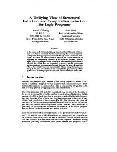
Phylogenies, or evolutionary trees, are a standard model to represent the evolutionary history of a set of species and are an indispensable tool in evolutionary biology [30]. In such a tree, extant species are represented as leaves, common ancestors are represented as internal nodes above a set of species, and the universal common ancestor of the species is represented as the root of the tree. The distance between two nodes in an evolutionary tree represents evolutionary distance such as time or number of mutations. An example of such a tree is shown in Figure 1.1. This is an example (brief and high-level) phylogenetic tree of life. It represents a hypothesis about the evolution of life on Earth. This hypothesis includes the relative similarity of any two species. Earlier work on the tree of life used morphology, or structural characteristics of species, to determine their similarity. However, advances in molecular biology have allowed species to be compared based on genetic information. The tree of life in Figure 1.1 splits organisms into three groups, Bacteria, Eukaryotes and Archaea. Prokaryotes, such as Bacteria and Archaea, tend to be smaller and less complex than Eukaryotes, such as most plants and animals. Molecular phylogenetics is particularly useful in the study of prokaryotic evolution due to the high rate of evolution and subtle differences in appearance of microscopic organisms. Phylogenetics is not limited to building trees of life. The methods of building and comparing phylogenies are relevant to diverse tasks such as vaccine design [15, 28, 37], haplotyping [18, 22], and even understanding the evolution of human language [21, 43]. Phylogenetics is a crossroads between mathematics, statistics, computer science and biology with many uses, both theoretical and applied. Much of the field of phylogenetics is, however, focused on the reconstruction of the tree of life or its subtrees. Phylogenetic reconstruction of such trees from molecular information is an error-prone task. Error arises from the alignment of molecular sequences used to provide similarity information between the extant taxa, the chosen statistical models of evolution, and the sheer 1
2
Eukaryotes Animals
Bacteria
Archaea
Fungi
Plants
Figure 1.1: High-level view of a rooted tree of life number of potential trees. Unfortunately, most useful optimization criteria for creating phylogenies, such as maximum likelihood [1] and Steiner tree [20], are NP-hard, and thus computationally intractable in most cases. In addition, it is often difficult to determine the common ancestor of all extant taxa in a given phylogenetic tree, represented as the root of the tree, without additional information, such as a known outgroup species. In such a case, phylogenetic inference algorithms generate unrooted trees. Such trees leave ancestor-descendant relationships undetermined, yet still contain evolutionary similarity and speciation information. Unfortunately, even good phylogenetic inference methods can not guarantee that a constructed tree correctly represents evolutionary history, since not all groups of species follow a simple treelike evolutionary pattern. Collectively known as reticulation events, non-tree-like evolutionary processes such as hybridization, horizontal gene transfer, and recombination result in species being composites of genes derived from different ancestors. Phylogenetic inference methods create a different phylogenetic tree for each such gene, representing the evolutionary story of that particular gene. To manage this effect, one can use phylogenetic distance metrics which determine how well the evolutionary hypotheses of two or more phylogenetic trees agree and often allow us to discover reticulation events where the hypotheses disagree. Assessing the quality of phylogenies proposed by approximate and heuristic phylogenetic inference methods often also requires measuring the similarity of many computed phylogenies. This is feasible only if distances under the used metric can be computed efficiently. Fast distance computations are also required for the analysis and visualization of tree space [3, 29].
3 A number of metrics are commonly used to define the distance between phylogenies. The Robinson-Foulds distance [39] is popular, as it can be calculated in linear time [17]. For this reason, this metric is well-suited to assessing phylogenies proposed by heuristics and for analyzing and visualizing tree space. Other metrics, such as the tree bisection and reconnection (TBR) and subtree prune and regraft (SPR) distances [30] and the hybridization number [4], are potentially more biologically meaningful but also significantly harder to compute. Given two trees on the same set of species but derived by analyzing different genes, the rooted SPR (rSPR) distance and the hybridization number of the two trees are important tools that often help to discover reticulation events. In particular, the rSPR distance provides a lower bound on the number of reticulation events [4, 6], and this metric has been regularly used to model reticulate evolution [33, 35]. The close relationship between rSPR operations and reticulation events has also led to advances in network models of evolution [4,14,35]. In these models, the evolutionary history of a set of taxa is represented by a network rather than a tree. A node of the network may have multiple parent nodes, as long as no cycles are induced. This can be used to model reticulation events since they result in multiple nodes providing genetic information to the same descendant. Much recent work has focused on computing the hybridization number between phylogenetic trees. One reason for this is that, while the rSPR distance between the trees also provides a lower bound on the hybridization number, the difference between the rSPR distance and the hybridization number may be arbitrarily large [4]. To model these distance metrics, we use the concept of rooted and unrooted maximum agreement forests (MAF’s) for SPR and TBR, and maximum acyclic agreement forests (MAAF’s) for hybridization number. An agreement forest of two phylogenies has the property that it can be obtained from either tree by cutting an appropriate set of edges. As such, it captures the parts of the evolutionary stories told by both trees that agree. By exploiting the relationship between agreement forests and SPR, TBR and hybridization, we reduce the dynamic problem of finding a sequence of SPR or TBR operations that transform one tree into the other into the static one of finding a set of edges to cut to obtain an MAF. Given an agreement forest between two trees T1 and T2 , a set of k rSPR (TBR in the unrooted case) operations that transform T1 into T2 can be easily recovered, where k is the number of edges removed to create the forest. A maximum agreement forest is such a forest where k is minimal.
4 This set of operations represents a possible set of reticulation events between the two trees. Similarly, given an acylic agreement forest between two trees T1 and T2 (a restriction of an agreement forest that disallows the donation of genetic information from descendant nodes to ancestor nodes and that represents the hybrid number), a hybrid network with that many hybridization events can be quickly constructed.
1.2
Related Work
While TBR distance, SPR distance, and hybridization number capture biologically meaningful notions of similarity between phylogenies, their practical use has been limited by the fact that they are NP-hard to compute [2, 12, 14, 27]. Thus, it is unlikely that any of these distances can be computed exactly with an algorithm that does not require exponential running time. There are three standard algorithmic approaches to such a problem. The first one is that of approximation algorithms. Such algorithms are generally efficient but do not guarantee that they find the correct answer. Rather, approximation algorithms provide a guaranteed bound on the ratio between the optimal solution and the one they compute, the approximation ratio. For example, a 3-approximation algorithm for a minimization problem is guaranteed to find a solution that is no smaller than the optimal answer and at most three times larger than that answer. See [42] for an introduction to approximation algorithms. Hein et al. [25] claimed a 3-approximation algorithm for computing SPR distances and introduced the notion of a maximum agreement forest (MAF) as the main tool underlying both the approximation algorithm and a proposed NP-hardness proof for computing SPR distances. The central claim was that the number of components in an MAF of two phylogenies is one more than the number of SPR operations needed to transform one into the other. Unfortunately, there were subtle mistakes in the proofs. Allen and Steel [2] proved that the number of components in an MAF is in fact one more than the TBR distance between the two trees. Rodrigues et al. [40] provided instances where the algorithm of [25] provides an approximation guarantee no better than 4 for the size of an MAF, thereby disproving the 3-approximation claim of [25]. They also proposed a modification to the algorithm, which they claimed to produce a 3-approximation for TBR. A counterexample to this claim was provided by Bonet et al. [9], who showed, however, that both the algorithms of [25] and [40] compute 5-approximations of the rSPR distance between two rooted phylogenies, and that the algorithms can be implemented in linear time. The approximation ratio
5 was improved to three by Bordewich et al. [11], but at the expense of an increased running time of O(n5 ).1 A second 3-approximation algorithm presented in [40] achieves a running time of O(n2 ). Using entirely different ideas, Chataigner [16] obtained an 8-approximation algorithm for TBR distances of two or more trees. There is no previous approximation algorithm for the hybridization number of two rooted phylogenies. A second algorithmic approach for solving NP-hard problems is that of fixed-parameter algorithms. The main idea of fixed-parameter algorithms is to restrict the combinatorial explosion in the running time to some function depending only on some parameter that is specific to the problem and independent of the input size. It is hoped that in a real application of this problem, the parameter is “relatively small” so that the exponential growth is reasonable. The fixed-parameter algorithm then efficiently solves the given parameterized problem. See [36] for an introduction to fixed-parameter tractability. For fixed-parameter algorithms that compute distance metrics on trees, the natural parameter is the distance under the given metric. In most biological datasets, we would expect (or hope) that the number of reticulation events is relatively small, and thus each of the distance metrics we consider would also be relatively small. For this reason, fixed-parameter algorithms can efficiently calculate these distance metrics despite the NP-hardness of these problems. The previously best fixed-parameter algorithm for rSPR distance is due to Bordewich et al. [11] and runs in O(4k · k4 + n3 ) time, where k is the distance between the two trees. For TBR distance, the previously best result is due to Hallett and McCartin [23], who provide an algorithm with running time O(4k · k5 + p(n)), where p(·) is a polynomial function. An earlier algorithm for this problem by Allen and Steel [2] had running time O(k3k + p(n)). For unrooted SPR, Hickey et al. [26] first claimed a fixed-parameter algorithm, but the correctness proof was flawed. Recently, St. John [41] proposed a correction of the central technical lemma in Hickey et al.’s result. In [13], Bordewich and Semple provided a fixed-parameter algorithm for the hybridization number of two rooted phylogenies with running time O((28k)k + n3 ). The final algorithmic approach is that of heuristic algorithms, of which we distinguish two types. The first type are similar to approximation algorithms in that they provide approximate solutions efficiently, but they do not provide a guaranteed approximation ratio. The second type of heuristic algorithms provide exact solutions with no guaranteed running time bound. 1 Using
non-trivial but standard data structures, the running time can be reduced to O(n4 ).
6 Approximation
FPT
TBR
Previous: 8-approx in polyn. time [16] New: 3-approx in linear time
Previous: O(4k k5 + p(n)) time [23] New: O(4k k + n3 ) or O(4k n) time
rSPR
Previous: 3-approx in O(n2 ) time [40] New: 3-approx in linear time
Previous: O(4k k4 + n3 ) time [11] New: O(3k k + n3 ) or O(3k n) time
Hybridization
Previous: — New: 3-approx in O(n log n) time
Previous: O((28k)k + n3 ) time [13] New: O(3k k log k + n3 ) or O(3k n log n) time
Table 1.1: Previous and new results on rSPR distance, TBR distance, and hybridization number. LatTrans by Hallet and Lagergen [24] models horizontal gene transfer events by a restricted version of rooted SPR operations, considering two ways in which the trees can differ. It computes the exact distance under this restricted metric with time complexity O(2k n2 ). HorizStory by Macleod et al. [32] supports multifurcating trees but does not consider SPR operations where the pruned subtree contains more than one leaf. EEEP by Beiko and Hamilton [6] performs a breadthfirst SPR search on a rooted start tree but performs unrooted comparisons between the explored trees and an unrooted end tree. The distance returned is not guaranteed to be exact due to optimizations and heuristics that limit the scope of the search, although EEEP provides options to compute the exact unrooted SPR distance with no guaranteed running time. More recently, RiataHGT by Nakhleh et al. [34] calculates an approximation of the SPR distance between rooted multifurcating trees in polynomial time.
1.3
Contribution
The contribution of this thesis is to develop more efficient methods to compute biologically meaningful distances between phylogenetic trees. We provide a unifying view on the approximation and FPT results discussed in the previous section and improve on them along the way, substantially in most cases. In particular, using a “shifting lemma” proved by Bordewich et al. [11], we show that the framework of the algorithms of [9, 25, 40] can be used not only to approximate the rSPR distance between two rooted phylogenies, but also to obtain approximation and FPT algorithms for rSPR distance, TBR distance, and hybridization number. Table 1.1 shows our new results in comparison to the best previous results. To the best of our knowledge, an approximation algorithm for hybridization number had not been obtained before. The 3-approximation algorithm for rSPR is the algorithm of Rodrigues et al. [40], with modifications to reduce its running time to linear and
7 to compute an MAF in addition to its size. We believe that the correctness proof obtained using our approach is simpler than the one presented in [40]. In addition to these theoretical results, we have implemented and tested the approximation and fixed-parameter algorithms for the rooted SPR distance on the protein tree dataset of [6]. We show that the fixed-parameter algorithm can efficiently and exactly compute SPR distances as large as 20. In particular, we contrast our fixed-parameter algorithm, which solved 68 cases with distances ranging from 20 to 25, with that of the Efficient Evaluation of Edit Paths (EEEP) algorithm [6], which exactly solved distances as large as 3 and, with an additional partitioning heuristic (which recent work shows may be made exact), solved 5 cases with distances ranging from 21 to 24. The rest of the thesis is organized as follows. We present the necessary terminology and notation in Chapter 2. Chapter 3 presents the main structural theorems that are at the heart of both the approximation and fixed-parameter algorithms. Chapter 4 presents the approximation algorithms. Chapter 5 discusses how to turn the approximation algorithms into fixed-parameter algorithms based on bounded search trees. Chapter 6 discusses the implementation of the approximation and fixed-parameter algorithms for rooted SPR distance. In Chapter 7 we present concluding remarks and discuss avenues for future research.
Chapter 2 Background This chapter introduces the terminology and notation used throughout this thesis. We mostly follow the definitions from [2, 9, 11, 12, 40].
2.1
Graph Theory
A graph G is composed of a set of vertices V (G) and a set of edges E(G), where each edge is a pair (u, v) of vertices from V (G). These vertices are the endpoints of the edge and are adjacent to each other. We say that vertices u and v are both incident to the edge (u, v). A simple graph has no duplicate edges and no edges that have the same vertex for both its endpoints (loops). In an undirected graph, edge (u, v) is the same as (v, u), for all u, v ∈ V . In a directed graph, (u, v) ̸= (v, u), for all u, v ∈ V . The number of edges incident to a vertex is called the degree of the vertex, deg(v). A sequence of vertices v1 , v2 , . . . , vn such that (vi , vi+1 ) is an edge, for each i ∈ {1, 2, . . . , n − 1}, is called a path. If v1 = vn , then it is also a cycle. The sequence of edges may also be referred to using these terms. For each pair of vertices in a connected graph, there is a path joining those vertices. A subgraph of a graph G has vertex and edge sets that are subsets of V (G) and E(G). For a graph G with n vertices, the following are equivalent: 1. G is a tree. 2. G is connected and has no cycles. 3. G is connected and has n − 1 edges. 4. G has n − 1 edges and no cycles. 5. G has no loops and contains, for each u, v ∈ V (G), a unique path from u to v. 8
9 A binary tree is a tree with maximum degree 3. Vertices of degree 1 are leaves, all other vertices are internal vertices. A forest is a simple, acyclic graph (its components are trees). In a rooted tree, one vertex is called the root and is not generally considered a leaf even if it is of degree 1. Edges are directed away from the root. This gives rise to the following relationships between vertices. If (u, v) is an edge, then u is called the parent of v, and v is called the child of u. If there is a directed path from vertex u to vertex v, then u is an ancestor of v and v is a descendant of u. Rooted trees are generally drawn so that parents are either above or below their children. In such cases the direction of edges is assumed and not shown. Deleting a vertex v from a graph G produces the graph G − v obtained by removing the vertex v from V (G) and every edge incident to v from E(G). Deleting an edge e from G produces the graph G − e obtained by removing e from E(G). Contracting an edge e from G deletes the edge and then merges its endpoints u and v into a single vertex u′ . Every edge incident to u or v becomes incident to u′ . 2.2
Phylogenetic Trees
An unrooted binary phylogenetic X-tree is a tree T whose leaves are the elements of a set X and each of whose internal nodes has degree three. We refer to these trees simply as (unrooted) X-trees. The set X is called the label set of T and contains the taxa whose evolutionary relationship the tree represents. When referring to multiple trees or forests of trees G, we use XG to refer to the label set of G. For a subset V of X, we use T (V ) to denote the smallest subtree of T that connects all nodes in V ; see Figure 2.1(b). A forced contraction replaces a vertex x of degree two and its two incident edges (w, x) and (x, v) with a single edge (w, v). The V -tree induced by T is the tree T |V obtained from T (V ) by splicing out all nodes of degree two using forced contractions. This captures the relationships between the leaves of T (V ) in the form of a minimal binary tree; see Figure 2.1(c). 7
7
1
6
2 3
5 4
(a)
2 3
5 4
(b)
7
2 3
5 4
(c)
Figure 2.1: (a) An X-tree T . (b) The subtree T (V ) for V = {2, 3, 4, 5, 7}. (c) The tree T |V obtained by forced contractions on T (V ).
10
1
2
3 4 (a)
5
1
3 (b)
4
1
3 (c)
4
Figure 2.2: (a) A rooted X-tree T . (b) The subtree T (V ) for V = {1, 3, 4}. (c) The tree T |V obtained by forced contractions on T (V ). A rooted X-tree is obtained from an unrooted one, T , by subdividing one of T ’s edges, declaring the node this introduces to be the root, and defining parent-child and ancestor-descendant relations in the standard way with respect to the chosen root. T (V ) and T |V are defined for rooted X-trees in a manner analogously to that of unrooted X-trees. However, when constructing T |V from T (V ), forced contractions are never applied to the root. Additionally, if the root has degree 1, then it and its adjacent edge are removed and its child is made the new root. A rooted X-tree represents the same information as the corresponding unrooted X-tree, as well as these additional ancestor-descendant relationships. However, knowledge (or a guess) of the root node of the Xtree is required to infer these relationships, which is not always possible for representations of biological data.
2.3
Phylogenetic Tree Distance Metrics
As discussed in the introduction, several distance measures between X-trees have been defined in the literature, reflecting different biological concepts, such as horizontal gene transfers. Of interest here are distance measures based on subtree prune and regraft (SPR) and tree bisection and reconnection (TBR) operations. Given an X-tree T , an SPR operation cuts an edge xy in T , thereby dividing T into two subtrees Tx and Ty containing x and y, respectively. Then it subdivides an edge of Ty using a new vertex y′ and adds an edge between x and y′ to reconnect Tx and Ty . Finally, vertex y is removed using a forced contraction. A TBR operation also starts by cutting an edge xy, but it subdivides an edge in each of the two trees, Tx and Ty , and then adds an edge x′ y′ to reconnect Tx and Ty , where x′ and y′ are the two vertices created in Tx and Ty by these edge subdivisions. Vertices x and y are then removed using forced contractions. Figure 2.3 illustrates both operations.
11 7
1
6
y0 x
6 5
7
2
7
1
5
y0
4
6
2
xy
3
6
2
y x
3
7
1
5
5
y0
4
3
2
y0 x0
6
4
Move one endpoint
Contract degree-2 vertices
7
2
y x
3
4
1
1
x0
3 4
5 Contract degree-2 vertices
Move both endpoints
SPR
TBR
Figure 2.3: Illustration of TBR and SPR operations. While TBR operations seem inherently unrooted, as applying such an operation to a rooted tree would require rerooting at least part of the tree, SPR operations translate naturally to the rooted case: a rooted SPR (rSPR) operation performs the same transformation as an SPR operation for unrooted trees; however, in the description of the operation above, vertex y is chosen to be the parent of vertex x. Thus, rSPR operations leave ancestor-descendant relations in the two subtrees intact. Moreover, at the end of the operation, forced contractions are applied only to non-root nodes of degree two, and the root is removed if edge xy was one of its incident edges, thereby making its child the new root of the tree.
y x 1
y0
y0
y x 2
3
4
5
3
4
1
x 2
5
3
4
1
2
5
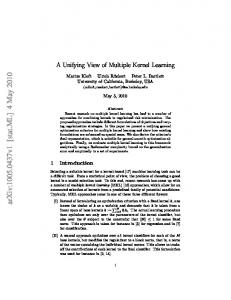
Figure 2.4: An rSPR operation on an X-tree T that regrafts edge e onto the edge above the leaf with label 5. TBR, SPR, and rSPR operations define distance measures dTBR (·, ·), dSPR (·, ·), and drSPR (·, ·) between (unrooted or rooted) X-trees, where the distance between two trees is the number of such operations required to transform one into the other. A related distance measure for rooted X-trees is their hybridization number, hyb(T1 , T2 ). This distance is defined in terms of hybrid networks of the two trees, where a hybrid network of T1 and T2 is a directed acyclic graph H such that both T1 and T2 can be obtained from H by deleting edges and performing forced contractions (H is said to display T1 and T2 ). See Figure 2.5. For a vertex x ∈ H, let degin (x) be its in-degree and deg− in (x) = max(0, degin (x) − 1). Then the hybridization number of T1 and T2 is minH ∑x∈H deg− in (x), where the minimum is taken over all hybrid networks H of T1 and T2 .
12
1
2
4
3
5
6
1
2
4
3
5
6
1
2
4
3
T2
T1
5
6
H
Figure 2.5: Two rooted X-trees T1 and T2 and a hybrid network H of them with the minimum hybrid number, 4. 2.4
Maximum Agreement Forests
TBR distance, rSPR distance, and hybridization number are known to be one less than the number of connected components in appropriately defined maximum agreement forests (MAF’s) [2, 4, 12]. To define these MAF’s, we first introduce some terminology. Given a forest F and a subset E of its edges, we write F − E to denote the forest obtained by deleting the edges in E from F. If forest F has components T1 , T2 , . . . , Tk with label sets X1 , X2 , . . . , Xk , we say that forest F yields forest F ′ if F ′ has components T1′ , T2′ , . . . , Tk′ (some of them possibly empty) and, for all 1 ≤ i ≤ k, Ti′ = Ti |Xi ; if all nodes of a component Ti are unlabelled (that is, Xi = 0), / we define Ti |Xi = 0. / For an X-tree T , we say that F is a forest of T if there exists a subset E of T ’s edges such that T − E yields F. Given two X-trees T1 and T2 and two forests F1 of T1 and F2 of T2 , a forest F is an agreement forest of F1 and F2 if there exist edge sets E1 and E2 such that F1 − E1 and F2 − E2 yield F; see Figure 2.6. Forest F is a maximum agreement forest (MAF) if there is no agreement forest of F1 and F2 with fewer connected components than F. We use m(F1 , F2 ) to denote the number of connected components in an MAF of F1 and F2 and e(F1 , F2 , F) to denote the size of the smallest 7
5
1
1
1 6
2
7
7
2
2 4
3
6
6 3
5 5
3
4 T1
4 F
T2
Figure 2.6: Two X-trees T1 and T2 and an agreement forest F of T1 and T2 . F is obtained from each tree by cutting the dashed edges.
13 edge set E such that F − E yields an agreement forest of F1 and F2 . In this thesis, F will always be a forest of F2 . The following theorem by Allen and Steel [2] establishes the relationship between TBR distances and unrooted MAF sizes. Theorem 2.1. For two unrooted X-trees T1 and T2 , dTBR (T1 , T2 ) = e(T1 , T2 , T2 ) = m(T1 , T2 ) − 1. In the rooted case, MAF’s are similarly related to rSPR distances. This, however, is true only if the MAF is defined with respect to augmented versions of the two trees, obtained by adding a new root node with label ρ to both trees and making the original root of each tree the child of ρ . An agreement forest of two forests F1 and F2 of T1 and T2 is then defined as a collection {Tρ′ , T1′ , T2′ , . . . , Tk′ } of rooted trees with label sets Xρ , X1 , X2 , . . . , Xk that satisfy the following conditions [12]: 1. The label sets Xρ , X1 , X2 , . . . , Xk partition X ∪ {ρ }, and ρ ∈ Xρ . 2. For all i ∈ {ρ , 1, 2, . . . , k}, Ti′ = F1 |Xi = F2 |Xi in the rooted sense. 3. The graphs in each of the sets {F1 (Xi ) | i ∈ {ρ , 1, 2, . . . , k}} and {F2 (Xi ) | i ∈ {ρ , 1, 2, . . . , k}} are vertex-disjoint trees. An MAF is again one with the minimum number of connected components. See Figure 2.7. Bordewich and Semple [12] proved the following theorem, where m(F1 , F2 ) and e(F1 , F2 , F) are defined as in the unrooted case. Theorem 2.2. For two rooted X-trees T1 and T2 , drSPR (T1 , T2 ) = e(T1 , T2 , T2 ) = m(T1 , T2 ) − 1.
ρ
ρ x
y
ρ y
y x
x 1
ρ
2
3 4 T1
5
6
1
2
3 4 T2
5
6
1
2
3 4 5 MAF
6
1
2
3 4 5 MAAF
6
Figure 2.7: Two rooted X-trees T1 and T2 , a maximum agreement forest of the two trees, and a maximum acyclic agreement forest of the two trees. Nodes x and y of the MAF form a cycle, and can be mapped to the shown nodes of T1 and T2 .
14 The hybridization number of two rooted X-trees T1 and T2 corresponds to an MAF of the two trees with an additional constraint. For two forests F1 and F2 of T1 and T2 , an agreement forest F of F1 and F2 is said to contain a cycle if there exist two nodes x and y that are roots of trees in F and such that x is an ancestor of y in T1 , while y is an ancestor of x in T2 . (Each node x in F can be mapped to nodes ϕ1 (x) in T1 and ϕ2 (x) in T2 by defining Xx to be set of labelled descendants of x in F and defining ϕi (x) to be the lowest common ancestor in Ti of all nodes in Xx .) An acyclic agreement forest is an agreement forest that contains no cycles. A maximum acyclic agreement forest (MAAF) of F1 and F2 is an agreement forest with the minimum number of connected components among all acyclic agreement forests of F1 and F2 . Figure 2.7 demonstrates these concepts, showing two trees T1 and T2 , a maximum agreement forest of T1 and T2 that contains a cycle with nodes x and y, the mapping of x and y to nodes in T1 and T2 , and a maximum acylic agreement forest of T1 and T2 . We denote the size of an MAAF of F1 and F2 by m(F ¯ 1 , F2 ) and the number of edges that need to be cut in a forest F of F2 to obtain such a forest by e(F ¯ 1 , F2 , F). The following result by Baroni et al. [4] relates e(T ¯ 1 , T2 , T2 ) to hyb(T1 , T2 ). Theorem 2.3. For two rooted X-trees T1 and T2 , hyb(T1 , T2 ) = e(T ¯ 1 , T2 , T2 ) = m(T ¯ 1 , T2 ) − 1. By Theorems 2.1–2.3, it suffices to compute or approximate the size of the right kind of MAF in order to compute or approximate the distance of two trees under one of the three metrics, dTBR (·, ·), drSPR (·, ·) or hyb(·, ·). Thus, we focus on MAF’s in the remainder of this thesis. For a forest F and two nodes a and b of F, we write a ∼F b to indicate that a and b belong to the same connected component of F, that is, there exists a path from a to b in F. Now, consider two forests F1 and F2 . Let a and c be vertices of F1 that share a common neighbour rac . We denote the edge from a to rac by ea and the edge from c to rac by ec . We denote with A the subtree of F1 induced by a and all nodes a′ such that edge ea belongs to the path from a′ to rac . The corresponding subtree of F1 induced by c and ec is denoted C. We call (a, c) a sibling pair if A and C also exist in F2 , that is, if there exist subtrees A′ and C′ of F2 isomorphic to A and C and such that the bijections between A and A′ and C and C′ respect leaf labels. 1 In
1
previous work, elements of a sibling pair (a, c) were required to be leaves. Similar algorithms are concerned only with MAFs and, thus, could contract sibling pairs (a, c) that exist in both forests F1 and F2 (that is, remove the leaves a and c and label their parent rac “(a,c)”). However, we have an additional constraint when dealing with an MAAF, in that cycles are relative to the original trees T1 and T2 and not the forests of them, F1 and F2 . Thus, we can not contract sibling pairs of these forests without potentially reducing e(T ¯ 1 , T2 , F2 ). Note that A and C can be reduced to the nodes a and c by repeated contraction of identical sibling pairs. Thus, our definition of sibling pairs captures the same structural properties of F1 and F2 as the one used in previous work, but without altering F1 or F2 .
15 2.5
Fixed-parameter tractability
Fixed-parameter algorithms, similar to approximation algorithms, are a tool for solving NP-hard problems. However, they provide exact solutions, which implies that exponential running times are unavoidable unless P = NP. Parameterized complexity, the mathematical tool behind fixed-parameter algorithms, was formalized by Downey and Fellows and co-authors in the 1990’s [19]. The material studied in this thesis uses this theory where necessary but uses an application-oriented look at the use and design of fixed-parameter algorithms. Fixed-parameter algorithms provide two advantages over approximation algorithms and heuristics; they guarantee the optimality of the given solution and they provide provable upper bounds on their computational complexity. The disadvantage of fixed-parameter algorithms is that exponential running times are expected. Parameterized algorithm design searches for a parameter such that the difficult part of the problem can be confined to the parameter. In practice, that parameter may be much smaller than the input size. NP-hard problems are generally phrased as decision problems, where the solution is either yes or no (i.e., is there a solution of size k). The corresponding optimization problem (i.e., find a solution of size k) is generally easily solved by an algorithm that solves the decision problem. A decision problem is fixed-parameter tractable if it can be determined in f (k) · nO(1) time whether or not a solution of size k exists, where f is a computable function only depending on k. The corresponding complexity class is called FPT. There are two main techniques that can be combined to create a fixed-parameter algorithm: kernelization and depth-bounded search trees. Reducing a problem to a “problem kernel”, or kernelization, uses reduction rules to replace, in polynomial time, the original instance of a problem with a reduced instance and reduced parameter such that the answer to the reduced instance is yes if and only if this is the case for the original instance. The size of the reduced instance depends only on the parameter k. Depth-bounded search trees are based on the idea of performing an exhaustive search for a solution. This exhaustive search is modelled as a tree, with each child of a node representing one possible next step from the state represented by the node. In a depth-bounded search tree, every step reduces the parameter k by at least one, so that a solution of size k exists if and only if there exists a path of length at most k from the root of the tree to a solution state with a nonnegative
16 parameter. Hence, only paths of length up to k need to be explored. Together with a bound on the branching factor of the tree, this gives a bound depending only on k on the number of configurations to be searched. If there is a reduction to a problem kernel and a depth-bounded search tree method for a particular problem, we can reduce the problem and then apply the bounded search tree method, which often leads to more efficient algorithms.
Chapter 3 The Structure of Agreement Forests This chapter presents the structural results that provide the intuition and correctness proofs for the algorithms presented in Chapters 4 and 5. All these algorithms start with a pair of trees (T1 , T2 ) and then cut edges, remove agreeing components from consideration, and merge sibling pairs in both trees until they are identical. The intermediate state is that T1 has been reduced to a forest F1 and T2 has been reduced to a forest F2 . F1 consists of a tree T˙1 and a set of components F that exist in F2 ; F2 consists of a set of components F˙2 that may not agree with F1 and the forest F that exists in F1 . The key part of each iteration is deciding which edges in F˙2 to cut next. The results in this chapter identify small edge sets in F˙2 such that at least one edge in each of these sets has the property that cutting it reduces e(T1 , T2 , F2 ) by one (or e(T ¯ 1 , T2 , F2 ) in the case of the MAAF algorithm). The approximation algorithm cuts all edges in the identified set, and the size of the edge set cut in each step gives the approximation ratio of the algorithm. The FPT algorithm tries each edge in the set in turn, so that the size of the set gives the branching factor for a bounded search tree algorithm. 3.1
Preliminaries
The following lemma by Bordewich et al. [11] is the central tool used in all our proofs. They proved this result for rooted trees. Here we argue that it also holds for unrooted trees. (This is essentially trivial, but we include the proof for completeness.) This lemma is illustrated in Figure 3.1. Lemma 3.1 (Shifting Lemma). Let T be an X-tree, F a forest of T , e and f edges in the same component of F, and E a subset of edges of F such that f ∈ E and e ∈ / E. Let v f be the end-vertex of f closest to e, and ve an end-vertex of e. If 1. v f ∼F−E ve , and 2. x �F−(E∪{e}) v f , for all x ∈ X, then F − E and F − (E \ { f } ∪ {e}) yield the same forest.1 1 In
the rooted case, it is assumed that ρ ∈ X.
17
18 x
f
ve
vf
e
y
x
f
ve
vf
y
e
(a)
(b)
Figure 3.1: (a) An illustration of the shifting lemma. Dashed lines indicate edges in E. (b) A case where the shifting lemma does not apply. The path from x to y in F − E includes f but not e. Proof. We show that x ∼F−E y if and only if x ∼F−(E\{ f }∪{e}) y, for all x,y ∈ X, and thus F − E and F − (E \ { f } ∪ {e}) yield the same forest. First suppose that x ∼F−E y but x �F−(E\{ f }∪{e}) y. Then e is on the path from x to y in F − E and f is not. By (1), v f ∼F−E ve , and thus either x ∼F−(E∪{e}) v f or y ∼F−(E∪{e}) v f . However, this contradicts (2). Now, suppose that x �F−E y, but x ∼F−(E\{ f }∪{e}) y. Then f is on the path from x to y in F − (E \ { f } ∪ {e}) and e is not. But then either x ∼F−(E∪{e}) v f or y ∼F−(E∪{e}) v f , which again contradicts (2). See Figure 3.1(b). The second tool we need is an observation that relates incompatible triples and quartets to agreement forests. A triple ab|c in a rooted tree T is defined by three leaves a, b, c such that the path from a to b is vertex-disjoint from the path from c to the root. We say a triple ab|c is incompatible with a forest F if its leaves either do not all belong to the same component of F or define a different triple, such as ac|b. See Figure 3.2(a). A quartet ab|cd in an unrooted tree T is defined by four leaves a, b, c, d such that the two paths from a to b and from c to d are vertexdisjoint. We say a quartet ab|cd is incompatible with a forest F if its leaves either do not all belong to the same component of F or define a different quartet, such as ac|bd. See Figure 3.2(b). Observation 3.2. (i) Let T1 and T2 be two rooted X-trees. Let F1 be a forest of T1 and F2 a forest of T2 . Let F be an agreement forest of F1 and F2 (and thus an agreement forest of T1 and T2 ). If ab|c is a triple of F1 incompatible with F2 , then either a �F b or a �F c. (ii) Let T1 and T2 be two unrooted X-trees. Let F1 be a forest of T1 and F2 a forest of T2 . Let F be an agreement forest of F1 and F2 . If ab|cd is a quartet of F1 incompatible with F2 , then a �F b, a �F c or c �F d.
19
b
a
d
b
d
c
a
c
a
b
c
c
a
b
(a)
(b)
Figure 3.2: (a) Incompatible triples. (b) Incompatible quartets. Finally, we require the following lemma, which shows that an agreement forest of T1 and T2 is also an agreement forest of the forests F1 of T1 and F2 of T2 that the algorithms construct. Lemma 3.3. Let T1 and T2 be two X-trees, F1 and F2 forests of T1 and T2 , respectively, and assume that F1 is the union of trees T˙1 , T˙2 , . . . , T˙k , while F2 is the union of forests F˙1 , F˙2 , . . . , F˙k such that XT˙i = XF˙i , for all 1 ≤ i ≤ k. If F2 − E yields an agreement forest of T1 and T2 , this is also an agreement forest of F1 and T2 . Proof. Let F ′ be the forest yielded by F2 − E. It suffices to show that there exists an edge set E1 such that F1 − E1 yields F ′ . Since F ′ is a forest of T1 , there exists a set E1′ of edges such that T1 − E1′ yields F ′ . We choose E1 to be the subset of edges in E1′ that are present in F1 . Now it suffices to prove that x ∼F1 −E1 y if and only if x ∼T1 −E1′ y, for all x, y ∈ X.
If x ∼F1 −E1 y, then none of the edges on the path from x to y in F1 belongs to E1′ . This path also
exists in T1 because F1 is a forest of T1 . Hence, x ∼T1 −E1′ y. If x �F1 −E1 y, we distinguish two cases. If x, y ∈ T˙i , for some 1 ≤ i ≤ k, then there exists an edge e ∈ E1 on the path from x to y in T˙i . Since E1 ⊆ E1′ , we have e ∈ E1′ , and x �T −E ′ y. If x ∈ T˙i 1
1
and y ∈ T˙j , for i ̸= j, then x ∈ F˙i and y ∈ F˙j . Hence, x �F ′ y. This implies that x �T1 −E1′ y because T1 − E1′ yields F ′ .
Now let T1 and T2 be X-trees, F1 a forest of T1 and F2 a forest of T2 . Assume that F1 consists of a tree T˙1 and a set of connected components F that exist in F2 . Then F2 can be divided into two sets: F and a set of components F˙2 . Let a and c be a sibling pair of T˙1 and assume that a and c do not share a parent in F2 , and neither is a root of a component of F2 . This implies that a and c are in F˙2 .
20 ρ
ρ rabc
rac ea ec a c A C T˙1
rab c ec ea eb a bC A B F˙2
(a)
rac ea ec a c A C T˙1
ea eb a b A B F˙2
ec c C
(b)
Figure 3.3: Tree labels for the rooted case: (a) a ∼F2 c, (b) a �F2 c.
In the rooted case, the sibling b of a in F2 is the other child of a’s parent. In the unrooted case, if a and c belong to the same tree of F2 , the sibling b of a in F2 is the node adjacent to a’s neighbour that does not belong to the path from a to c in F2 . Otherwise, b is any node at distance two from a in F2 . Note that b is not necessarily a leaf. We use ea and eb to denote the edges connecting a and b to their common neighbour rab , and B to denote the subtree of F2 induced by all nodes b′ such that edge eb belongs to the path from b′ to rab . The sibling d of c and its attached subtree D are defined analogously. In the rooted case, rab is the parent of a and b and, if a and c belong to the same component of F2 , we assume that the distance from the root of the component to a is no less than the distance from the root to c, which implies that b does not belong to the path from a to c in F2 . 3.2
Rooted MAF
With these tools in hand, we are now ready to prove three results characterizing edges that need to be cut in order to make progress towards an M(A)AF. The first result considers rooted MAF’s and shows that at least one of the edges ea , eb , and ec has the property that cutting it reduces e(T1 , T2 , F2 ) by one. Theorem 3.4. Let T1 and T2 be two rooted X-trees, and let F1 be a forest of T1 and F2 a forest of T2 . Suppose that F1 consists of a tree T˙1 and a set of components F that exist in F2 . Let (a, c) be a sibling pair of T˙1 . Finally, suppose that a and c do not share a parent in F2 , and neither is the root of a component of F2 . Then e(T1 , T2 , F2 − {ex }) = e(T1 , T2 , F2 ) − 1, for some x ∈ {a, b, c}.
21 Proof. It suffices to prove that there exists an edge set E such that F2 − E yields an MAF of T1 and T2 and E ∩ {ea , eb , ec } ̸= 0. / So let E be chosen such that F2 − E yields an MAF F ′ and assume that E ∩ {ea , eb , ec } = 0. / By Lemma 3.3, F ′ is also an agreement forest of F1 and F2 . We prove that there exists an edge f ∈ E such that F2 − E and F2 − (E \ { f } ∪ {ex }) yield the same forest, for some x ∈ {a, b, c}. Thus, since F2 − E yields an MAF, so does F2 − E ′ , where E ′ = E \ { f } ∪ {ex }, and E ′ ∩ {ea , eb , ec } = ̸ 0. / First suppose there exists no leaf b′ ∈ B such that b′ ∼F2 −E rab . Then we can choose an arbitrary leaf b′ ∈ B and let f be the first edge in E on the path from rab to b′ . Now let e = eb , and choose vertices ve and v f as in Lemma 3.1. The choice of edge f and the fact that e ∈ / E ensure that v f ∼F2 −E ve . Together with the fact that b′′ �F2 −E rab , for all b′′ ∈ B, this implies that x �F2 −(E∪{e}) v f , for all x ∈ X ∪ {ρ }. Thus, Lemma 3.1 applies to edges f and eb , and we can replace f with eb in E without altering the forest yielded by F2 − E. Similarly, if there exists no leaf a′ ∈ A such that a′ ∼F2 −E rab , then we can choose an arbitrary leaf a′ ∈ A and replace the first edge in E on the path from rab to a′ with ea in E without altering the forest yielded by F2 − E. The same holds if there exists no leaf c′ ∈ C such that c′ ∼F2 −E c. So assume that there exist leaves a′ ∈ A, b′ ∈ B, and c′ ∈ C such that b′ ∼F2 −E rab , a′ ∼F2 −E rab , and c′ ∼F2 −E c. Hence, a′ ∼F2 −E b′ . Since (a, c) is a sibling pair in F1 that does not exist in F2 , we have a′ , b′ , c′ ∈ F˙2 and hence, a′ , b′ , c′ ∈ T˙1 ; this implies that a′ c′ |b′ is a triple of F1 . On the other hand, c ∈ / B implies that either a′ b′ |c′ is a triple of F2 or a′ �F2 c′ . In either case, the triple a′ c′ |b′ is incompatible with F2 . Since F2 − E yields an agreement forest F ′ of F1 and F2 and a′ ∼F2 −E b′ , Observation 3.2(i) now implies that a′ �F2 −E c′ , which, since a′ ∼F2 −E a and c′ ∼F2 −E c, implies that a �F2 −E c. Since (a, c) is a sibling pair of F1 and a ∼F2 −E b, a �F2 −E c implies that c is a root in F2 − E. Since c is not a root in F2 , there exists an edge f ∈ E outside C that belongs to the same connected component of F2 as c, and e = ec and f satisfy Lemma 3.1 if f is chosen so that no edge on the path from f to c is in E. Hence, F2 − E and F2 − (E \ { f } ∪ {ec }) yield the same forest. We require the following corollary for the approximation algorithm, which simply shows that cutting ea , eb and ec reduces e(T1 , T2 , F2 ) by at least 1. Corollary 3.5. Let T1 and T2 be two rooted X-trees, and let F1 be a forest of T1 and F2 a forest of T2 . Suppose that F1 consists of a tree T˙1 and a set of components that exist in F2 . Let (a, c) be a sibling pair of F1 that is not a sibling pair of F2 , and assume that neither a nor c is the root of a component of F2 . Then e(T1 , T2 , F2 − {ea , eb , ec }) ≤ e(T1 , T2 , F2 ) − 1.
22 a ea rab
A C
A a ea
b eb
B
c ec
rcd ec
ed
c
d
C
D
T˙1
F˙2
Figure 3.4: Tree labels for the unrooted case where a ∼F2 c. Note that Theorem 3.4 also holds if we replace e(T1 , T2 , ·) with e(T ¯ 1 , T2 , ·). To see this, it suffices to consider a set E in the proof such that F − E yields an MAAF instead of an MAF. The proof only relies on F − E yielding an agreement forest. Thus, we have the following corollary. Corollary 3.6. Let T1 and T2 be two rooted X-trees, and let F1 be a forest of T1 and F2 a forest of T2 . Suppose that F1 consists of a tree T˙1 and a set of components that exist in F2 . Let (a, c) be a sibling pair of T˙1 that is not a sibling pair of F2 , and assume that neither a nor c is the root of a component of F2 . Then 1. e(T ¯ 1 , T2 , F2 − {ex }) = e(T ¯ 1 , T2 , F2 ) − 1, for some x ∈ {a, b, c}. 2. e(T ¯ 1 , T2 , F2 − {ea , eb , ec }) ≤ e(T ¯ 1 , T2 , F2 ) − 1.
3.3
Unrooted MAF
The next theorem provides an analogous result to Theorem 3.4 for unrooted MAF’s. Theorem 3.7. Let T1 and T2 be two unrooted X-trees, and let F1 be a forest of T1 and F2 a forest of T2 . Suppose that F1 consists of a tree T˙1 and a set of components that exist in F2 . Let (a, c) be a sibling pair of T˙1 . Finally, suppose that a and c do not share a neighbour in F2 , and neither F2 |XA nor F2 |XC is a component of F2 . Then e(T1 , T2 , F2 − {ex }) = e(T1 , T2 , F2 ) − 1, for some x ∈ {a, b, c, d}.
23 Proof. As in the proof of Theorem 3.4, our goal is to show that there exists a set E such that F2 − E yields an MAF of T1 and T2 and E ∩ {ea , eb , ec , ed } = ̸ 0. / Again, we show that, if F2 − E yields an MAF F ′ of T1 and T2 and E ∩ {ea , eb , ec , ed } = 0, / we can find an edge f ∈ E and an x ∈ {a, b, c, d} such that F2 − E and F2 − (E \ { f } ∪ {ex }) yield the same forest. By the same arguments as in the proof of Theorem 3.4, if there exists no leaf b′ ∈ B such that b′ ∼F2 −E rab , then we can choose an arbitrary leaf b′ ∈ B and replace the first edge in E on the path from rab to b′ with eb in E without altering the forest yielded by F2 − E. The same holds if there exists no leaf a′ ∈ A such that a′ ∼F2 −E rab , c′ ∈ C such that c′ ∼F2 −E rcd , or d ′ ∈ D such that d ′ ∼F2 −E rcd . So assume that there exist leaves a′ ∈ A, b′ ∈ B, c′ ∈ C, and d ′ ∈ D such that a′ ∼F2 −E rab , b′ ∼F2 −E rab , c′ ∼F2 −E rcd and d ′ ∼F2 −E rcd . Hence, b′ ∼F2 −E a′ and d ′ ∼F2 −E c′ . Since (a, c) is a sibling pair of F1 , a′ c′ |b′ d ′ is a quartet of F1 , while c ∈ / B implies that either a′ b′ |c′ d ′ is a quartet of F2 or a �F2 c. In either case, the quartet a′ c′ |b′ d ′ is incompatible with F2 . Since F2 − E yields an agreement forest of T1 and T2 , it also yields an agreement forest of F1 and F2 , by Lemma 3.3. Hence, as b′ ∼F2 −E a′ and d ′ ∼F2 −E c′ , Observation 3.2(ii) implies that a′ �F2 −E c′ , which, since a′ ∼F2 −E a and c′ ∼F2 −E c, implies that a �F2 −E c. Since (a, c) is a sibling pair of F1 and a ∼F2 −E b, a �F2 −E c implies that c′ �F2 −E x, for all x ∈ X \ XC . Since F2 |XC is not a component of F2 , this implies that there exists an edge f ∈ E that belongs to the same connected component of F2 as c′ and is not in C. Thus, if f is chosen so that none of the edges on the path from f to c is in E, edges e = ec and f satisfy Lemma 3.1, which implies that F2 − E and F2 − (E \ { f } ∪ {ec }) yield the same forest. Similar to Theorem 3.4, Theorem 3.7 immediately implies that e(T1 , T2 , F2 − {ea , eb , ec , ed }) ≤ e(T1 , T2 , F2 ) − 1. However, we can do a little better. Theorem 3.8. Let T1 and T2 be two unrooted X-trees, and let F1 be a forest of T1 and F2 a forest of T2 . Suppose that F1 consists of a tree T˙1 and a set of components that exist in F2 . Let (a, c) be a sibling pair of T˙1 that is not a sibling pair of F2 , and assume that a and c do not share a neighbour in F2 , and neither F2 |XA nor F2 |XC is a component of F2 . Then e(T1 , T2 , F − {ea , eb , ec }) ≤ e(T1 , T2 , F) − 1. Proof. Let E be an edge set such that F2 − E yields an MAF F ′ of T1 and T2 . We can again assume that E ∩ {ea , eb , ec } = 0, / as otherwise the theorem holds trivially. Moreover, by Lemma 3.3, F ′ is an agreement forest of F1 and F2 .
24 As in the proof of Theorem 3.7, if there exists no leaf b′ ∈ B such that b′ ∼F2 −E rab , then we can choose an arbitrary leaf b′ ∈ B and replace the first edge in E on the path from rab to b′ with eb without altering the forest yielded by F2 − E. The same holds if there exists no leaf a′ ∈ A such that a′ ∼F2 −E rab , or c′ ∈ C such that c′ ∼F2 −E rcd . So, we can again assume that there exist leaves a′ ∈ A, b′ ∈ B, and c′ ∈ C such that a′ ∼F2 −E rab , b′ ∼F2 −E rab and c′ ∼F2 −E rcd . Hence, b′ ∼F2 −E a′ . Next, we show that there exists an edge f ∈ E such that F2 − (E ∪ {ea , eb }) and F2 − (E \ { f } ∪ {ea , eb , ec }) yield the same forest. This forest is an agreement forest of T1 and T2 , as it can be obtained by cutting edges ea and eb in F ′ . Hence, e(T1 , T2 , F2 − {ea , eb , ec }) ≤ |E \ { f }| = |E| − 1 = e(T1 , T2 , F2 ) − 1. Note that this is not the same as claiming that we can replace an edge f ∈ E with an edge in {ea , eb , ec } without altering the resulting forest. It is crucial that all three edges are cut. We observe that (a, c) being a sibling pair in F1 and c ∈ / B imply that a′ c′ |b′ d ′ is a quartet of F1 incompatible with F2 , for all d ′ ∈ / XA ∪ XB ∪ XC . If a′ ∼F2 −E c′ , then a′ ∼F2 −E b′ and Observation 3.2(ii) imply that c′ �F2 −E d ′ , for all d ′ ∈ / XA ∪ XB ∪ XC . If a′ �F2 −E c′ , then a �F2 −E c. Since (a, c) is a sibling pair of F1 , this implies that the component of F ′ containing c′ contains no leaves not in XC . Hence, again c′ �F2 −E d ′ , for all d ′ ∈ / XA ∪ XB ∪ XC . Therefore, c′ �F2 −E ′ x, for all x ∈ X \ XC , where E ′ = E ∪ {ea , ec }. Since the component of F2 containing c′ contains at least one leaf x outside C, this implies that there exists an edge in E on the path from x to c′ outside C, and the closest such edge to c′ and edge e = ec satisfy the conditions of Lemma 3.1. Hence, F2 − (E ∪ {ea , eb }) and F2 − (E \ { f } ∪ {ea , eb , ec }) yield the same forest. 3.4
Rooted MAAF
While Theorem 3.4 suffices as a basis of an algorithm to compute or approximate an MAF of two rooted trees, a little extra work is required to obtain an MAAF. As observed in Corollary 3.6, we can use this theorem to make progress towards an MAAF until we obtain an agreement forest of the two trees. If this forest is in fact acyclic, we are done. Otherwise, we need to continue cutting edges to remove all cycles that may exist. The next theorem identifies candidate edges to cut. In this theorem, we consider two trees, A and B, of the agreement forest whose roots, a and b, form a cycle. We call (a, b) a cycle pair and use ea to denote any of the two edges in A incident to a, and eb to denote any of the two edges in B incident to b.
25 a
b eb
ea
A
B
Figure 3.5: Tree labels for a cycle pair. Theorem 3.9. Let T1 and T2 be two rooted X-trees, F an agreement forest of T1 and T2 , and (a, b) a cycle pair of F. Then e(T ¯ 1 , T2 , F − {ex }) = e(T ¯ 1 , T2 , F) − 1, for some x ∈ {a, b}. In particular, e(T ¯ 1 , T2 , F − {ea , eb }) ≤ e(T ¯ 1 , T2 , F) − 1. Proof. Once again, our goal is to show that there exists a set E of edges of F such that F − E yields an MAAF of T1 and T2 and E ∩ {ea , eb } ̸= 0. / So we choose E to be a set such that F − E yields an MAAF F ′ of T1 and T2 , and assume that E ∩ {ea , eb } = 0. / Let A1 and A2 be the two subtrees of A rooted in a’s children, and let B1 and B2 be the two subtrees of B rooted in b’s children. First observe that there exists an index i such that either a′ �F−E a, for all a′ ∈ XAi , or b′ �F−E b, for all b′ ∈ XBi . Indeed, if this was not the case, there would exist leaves a1 ∈ A1 , a2 ∈ A2 , b1 ∈ B1 , and b2 ∈ B2 such that a1 ∼F−E a2 and b1 ∼F−E b2 , which implies that both a and b exist in F ′ , and F ′ would not be acyclic. So assume w.l.o.g. that a′ �F−E a, for all a′ ∈ A1 . In this case, Lemma 3.1 states that, if we choose a leaf a′ ∈ A1 and the edge f ∈ E closest to a on the path from a to a′ , then F − E and F − (E \ { f } ∪ {ea }) yield the same forest, which is the MAAF F ′ . Hence, the edge set E ′ = E \ { f } ∪ {ea } has the property that F − E ′ yields an MAAF of T1 and T2 and E ′ ∩ {ea , eb } = ̸ 0. /
Chapter 4 Approximation Algorithms This chapter presents our approximation algorithms for computing rooted maximum agreement forests, unrooted maximum agreement forests, and rooted maximum acyclic agreement forests. These respectively provide approximations for the rooted SPR distance, TBR distance, and hybridization number between two phylogenies. The algorithms are based on applications of the theorems from Chapter 3.
4.1
3-Approximation for Rooted MAF (rSPR Distance)
The first algorithm we present is a 3-approximation algorithm for rooted MAF, that is, rooted SPR distance. This algorithm is essentially the one discussed in [40], modified to achieve linear time and to compute an MAF in addition to its size. We include it here to demonstrate that Theorem 3.4 establishes its correctness, and also as a basis for the other algorithms. The algorithm starts with a pair of trees (T1 , T2 ) and modifies both through a series of transformations. T1 and T2 are reduced to forests F1 and F2 . F1 consists of a tree T˙1 and a forest F. F2 consists of two forests, one F, the other a forest F˙2 with XT˙1 = XF˙2 . The algorithm maintains two sets of labelled nodes, Rt and Rd . Rd are the roots of trees in F. Rt are the roots of subtrees that agree between T˙1 and F˙2 . Initially, Rt = X and Rd = 0. / The goal is to identify agreeing components via Rt and move them to F by moving their roots to Rd . The algorithm terminates when Rt = 0, / at which point F is an agreement forest of T1 and T2 . The algorithm also maintains a counter, D, of the number of edges in T2 it has (i) (i) (i) (i) (i) (i) cut so far. We use F , F , T˙1 , F˙2 , R , Rt , and D(i) to denote the state of the algorithm after 1
2
d
the ith transformation. Each iteration applies one of the following cases, illustrated in Figure 4.1. 0. If |Rt | ≤ 2, then add F˙2 to F and set T˙1 = F˙2 = 0. / This is correct because F˙2 ⊆ T˙1 at this point, that is, F˙2 ∪ F is an agreement forest of F1 and F2 and, hence, of T1 and T2 . 26
27 1. As long as there is a node r ∈ Rt that is a root in F˙2 , we move it from Rt to Rd and cut its parent edge in T˙1 followed by a forced contraction. D remains unchanged. For the other two rules, the algorithm chooses a fixed sibling pair (a, c) in Rt . 2. If (a, c) is also a sibling pair of F˙2 , the algorithm removes a and c from Rt , labels their parent in both trees with (a, c), and adds it to Rt . 3. If (a, c) is not a sibling pair in F˙2 , then assume w.l.o.g. that a’s distance from the root of T2 is no less than that of c. Node a must have a sibling b in F˙2 because neither a nor c is a root in F˙2 (otherwise Case 1 would have moved them to Rd ). In this case, the algorithm cuts edges ea , eb , and ec in F˙2 , performs the necessary forced contractions and increases D by three. Theorem 4.1. Given two rooted X-trees T1 and T2 , we can compute a 3-approximation, in linear time, of e(T1 , T2 , T2 ) = drSPR (T1 , T2 ). Proof. We use the final value of D from the algorithm above as the approximation of e(T1 , T2 , T2 ). We argue below that the algorithm terminates, in linear time. If the algorithm terminates after k iterations, k′ of which change D, then its output is D(k) = 3k′ . We prove that e(T1 , T2 , T2 ) ≤ 3k′ ≤ 3e(T1 , T2 , T2 ), thereby proving that the value D(k) output by the algorithm is a 3-approximation of e(T1 , T2 , T2 ) = drSPR (T1 , T2 ). (i−1)
(i)
), because For every iteration that leaves D unchanged, we have e(T1 , T2 , F2 ) = e(T1 , T2 , F2 (i) only Cases 0, 1 and 2 leave D unchanged and these cases only change labels of F˙2 or move com(i−1) ponents from F˙2 to F (i) . Every iteration that changes D applies Case 3. In this case, (a, c) is a (i−1) (i) (i−1) (i−1) = = T˙1 ∪ F (i−1) is a forest of T1 , F sibling pair of T˙1 with subtrees A and C. Since F 2
1
(i−1) (i−1) F˙2 ∪ F (i−1) is a forest of T2 , (a, c) is not a sibling pair of F2 in this case and neither a nor c (i−1)
is a root of a component in F2
(i)
(i−1)
, Theorem 3.4 implies that e(T1 , T2 , F2 ) ≤ e(T1 , T2 , F2
) − 1.
Hence, we have e(T1 , T2 , T2 ) ≥ k′ , that is, D(k) = 3k′ ≤ 3e(T1 , T2 , T2 ). Conversely, since the 3k′ edges we cut in T2 yield an agreement forest F (k) of T1 and T2 , we have e(T1 , T2 , T2 ) ≤ 3k′ . To bound the running time of the algorithm, we observe that it terminates after O(n) iterations. Indeed, each iteration removes at least one of the O(n) vertices and edges in T1 or T2 from consideration through edge cuts or labelling ancestors. Moreover, T1 contains a sibling pair as long as T˙1 has size greater than 2, which implies that one of the transformation rules is applicable. Thus, it suffices to prove that each iteration can be implemented in constant time, which we do in Section 4.2. (The argument is similar to the one presented by Bonet et al. [9].)
28 ρ
ρ
c c T˙1
F˙2
T˙1
F˙2
(a) Case 1 ρ
ρ
rac a ˙ T1
rac c
a
(a, c) c F˙2
(a, c)
T˙1
F˙2
(b) Case 2 ρ
ρ rabc
rabc
rac a
rab c
a
T˙1
rac
c b
a
F˙2
T˙1
c c
a
b F˙2
(c) Case 3, a ∼T2 c ρ
ρ
rac a T˙1
rac c
a
b
c
F˙2
a T˙1
c
a
b
c
F˙2
(d) Case 3, a �T2 c
Figure 4.1: The three cases of the approximation algorithm for rooted MAF. Case 3 is split into two subcases depending on whether a and c belong to the same component of T2 .
29 4.2
Linear-Time Implementation of the Rooted MAF Approximation
In this section, we discuss how to represent the two forests in the rooted MAF approximation algorithm from Section 4.1 to ensure that each of the O(n) iterations of the algorithm takes constant time, resulting in a total running time of O(n) for the algorithm. We represent each tree as a collection of nodes, each of which points to its parent, left child, and right child. In addition, every labelled node stores a pointer to its counterpart in the other forest. This is initially done through a linear-time preprocessing step. For T˙1 , we maintain a list of sibling pairs, and every node of Rt stores a pointer to the pair it belongs to, if any. For F˙2 , we maintain a list of roots among the nodes of Rt . While the root list is non-empty, we remove its next element c. Given the above pointers, it takes constant time to identify node c in T˙1 and its parent, to remove c from T˙1 , F˙2 and Rt and put it into Rd , and splice out its parent in T˙1 . Thus, we can check in constant time whether Case 1 applies and, if so, apply it. If c belonged to a sibling pair in T˙1 , we can eliminate it from the list of sibling pairs. Moreover, c’s sibling a in T˙1 may now be the sibling of another node c′ ∈ Rt in T˙1 , and we may need to add the pair (a, c′ ) to the list of sibling pairs. This is the case if a’s new sibling c′ is labelled, which is also easily checked in constant time. This concludes the discussion of applying Case 1 in constant time. To implement Cases 2 and 3, we retrieve the next sibling pair (a, c) of T˙1 . The pair (a, c) is a sibling pair of F˙2 if and only if a and c have the same parent in F˙2 . This allows us to distinguish between Cases 2 and 3 in constant time. In Case 2, we remove a and c from Rt , set up pointers between the two parents in T˙1 and F˙2 , and add them to Rt . If rac has no parent in F˙2 , it is now a root and is added to the root list. Additionally, if rac has a labelled node a′ for a sibling in T˙1 , then (a′ , rac ) is a sibling pair in T˙1 , which must be added to the list of sibling pairs. In Case 3, we identify the sibling b of a in F˙2 by following two pointers. Then edges ea , eb , and ec can be removed in constant time. We need to add a and c to the list of roots, and also node b if it is labelled. Finally, we need to remove rab from F˙2 and splice out its parent, if any. The parent rc of node c also needs to be removed or spliced out, depending on whether it has a parent. Moreover, if rc is removed and the sibling d of c is labelled, then d is now a root and needs to be added to the root list. Again, all these are local pointer manipulations that can be carried out easily in constant time.
30 The last remaining issue is that, in Case 3, we are required to choose a and c so that the distance from a to the root r of T2 is no less than that from c to r when a ∼F˙2 c. After using a standard lineartime depth-first traversal of T2 to label all its nodes with their depths, we can choose a to be the node with the greater depth label in constant time in each application of Case 3. 4.3
3-Approximation for Unrooted MAF (TBR Distance)
The 3-approximation algorithm for unrooted MAF and, hence, for TBR distance is the same as for the rooted case, except that edges ea , eb , and ec in Case 3 are used in their unrooted meaning, and the algorithm may end up cutting not eb but the third edge apart from ea and eb incident to rab : 3. If (a, c) is not a sibling pair in T2 , let b∗ be one of the two nodes at distance two from a in T2 . Then the algorithm cuts edges ea , eb∗ , and ec in T2 and increases D by three. Note, that the algorithm treats the components of F˙2 that have been separated as rooted trees. This is not a problem, as we merely use these “roots” to keep track of the components. When we move such a “root” r from Rt to Rd , we contract it out so that F consists of unrooted trees that agree in both F1 and F2 . Thus, when the algorithm terminates and F˙2 is empty, F is an agreement forest of T1 and T2 . The different cases of the algorithm are illustrated in Figure 4.2. Theorem 4.2. Given two unrooted X-trees T1 and T2 , we can compute a 3-approximation of e(T1 , T2 , T2 ) = dTBR (T1 , T2 ) in linear time. Proof. The running time of the algorithm is established as in the rooted case. We prove that, if the algorithm runs for k iterations, the final value of D, D(k) , is a 3-approximation of e(T1 , T2 , T2 ). Again, let k′ be the number of applications of Case 3. Then D(k) = 3k′ . As in the proof of (i)
(i−1)
Theorem 4.1, each application of Cases 0, 1 and 2 satisfies e(T1 , T2 , F2 ) = e(T1 , T2 , F2 (i)
(i−1)
it suffices to prove that e(T1 , T2 , F2 ) ≤ e(T1 , T2 , F2
). Hence,
)−1 for each application of Case 3. If Case 3
cut edges ea , eb , and ec , this would follow from Theorem 3.8 similarly to the proof of Theorem 4.1. As pointed out, however, we may cut the third edge incident to rab instead of eb . The reason we do this is that this is much simpler than checking which of the two edges incident to rab apart from ea does not belong to the path from a to c (which would require extra preprocessing). To establish that (i)
(i−1)
e(T1 , T2 , F2 ) = e(T1 , T2 , F2
(i−1)
− {ea , eb∗ , ec }) ≤ e(T1 , T2 , F2
) − 1, we observe that, if b∗ ̸= b,
then edges e = eb∗ and f = eb satisfy Lemma 3.1 with respect to the edge set E = {ea , eb , ec }. (i−1)
Hence, F2
(i−1)
− {ea , eb , ec } and F2
(i)
− {ea , eb∗ , ec } yield the same forest, F2 .
31
c c
F˙2
T˙1
F˙2
T˙1
(a) Case 1
a
(a, c)
a
(a, c)
rac
c rac
c
rac
rac
T˙1
T˙1
F˙2
F˙2
(b) Case 2 a
a
b
a
a
c
b
c
c
c T˙1
F˙2
T˙1
F˙2
(c) Case 3, a ∼T2 c a
c
a
a
c a
b
b
c
T˙1
c
T˙1
F˙2
F˙2
(d) Case 3, a �T2 c
Figure 4.2: The three cases of the approximation algorithm for unrooted MAF. Case 3 is split into two subcases depending on whether a and c belong to the same component of T2 .
32 4.4
3-Approximation for Rooted MAAF (Hybridization Number)
The algorithm for approximating rooted MAAF consists of two stages. First we run the algorithm for rooted MAF to obtain an approximation F of an MAF of T1 and T2 . Given F, it remains to identify and break cycles. Whenever we cut an edge in the process, we increase D by one, starting with the value of D at the end of the MAF algorithm. Our algorithm maintains two sets, Rd and Rt , of roots of trees in F. The roots in Rd do not form cycles with each other. Rt contains roots that may be involved in cycles. Initially, Rd = 0/ and Rt contains all roots of trees in F. Each iteration of the algorithm removes a root b from Rt and tests whether b forms a cycle with a root a ∈ Rd . If not, we add b to Rd and move on to the next root in Rt . If there is a root a ∈ Rd such that (a, b) is a cycle pair, we remove one of the two edges incident to each of a and b and increase D by two. This breaks the two trees in F with roots a and b into two subtrees each; their roots are the children of a and b in F. We add a’s children to Rd and b’s children to Rt and then move on to the next iteration. The algorithm terminates when Rt = 0, / at which point F has been refined to an acyclic agreement forest of T1 and T2 . The total number of nodes added to Rt throughout the algorithm is at most the number of nodes in F, which is O(n). Hence, Rd also never has size greater than O(n), and checking every node in Rt against every node in Rd requires checking O(n2 ) pairs in total. It is trivial to check whether two nodes a and b form a cycle in O(n) time, giving a running time of O(n3 ) for the algorithm. In Section 4.5.1 we show how to check whether two nodes a and b form a cycle in O(1) time, for a running time of O(n2 ). In Section 4.5.2, we discuss how to reduce the running time to O(n log n) by taking a geometric view of the problem. Using the naive implementation, we have the following result. Theorem 4.3. Given two unrooted X-trees T1 and T2 , we can compute a 3-approximation of e(T ¯ 1 , T2 , T2 ) = hyb(T1 , T2 ) in O(n3 ) time. Proof. We have already discussed the running time of the algorithm. We first show that the algorithm computes an acyclic agreement forest of T1 and T2 . The first phase of the algorithm constructs an agreement forest of T1 and T2 , by Theorem 4.1. The second phase computes a refinement F ′ of F and, hence, an agreement forest of T1 and T2 . We argue that F ′ has no cycles. We add a root b ∈ Rt to Rd only if there is no root a ∈ Rd such that a and b form a cycle. When breaking a cycle pair (a, b), we add a’s children a1 and a2
33 to Rd without testing whether they form cycles with other roots in Rd . However, if there was a root c ∈ Rd such that ai and c form a cycle, then a and c would have had to form a cycle as well; otherwise, c would have to belong to the path from a to ai in one of T1 and T2 , and it couldn’t be the root of a tree. This shows that the roots in Rd do not form cycles with each other at any time. Since the algorithm terminates when all roots in F ′ are in Rd , F ′ is acyclic. To prove the approximation ratio, consider all iterations over the two phases of the algorithm. (i)
Each application of Cases 0, 1 and 2 of the first phase of the algorithm satisfies e(T1 , T2 , F2 ) = (i−1)
e(T1 , T2 , F2
(i)
(i−1)
), since F2 = F2
. In an iteration of the first phase of the algorithm that changes (i−1) (i−1) (i−1) ∪ F (i−1) of T1 and F2 = D, we have two rooted X-trees T1 and T2 and forests F1 = T˙1 (i−1) (i−1) that is not a sibling pair of ∪ F (i−1) of T2 . We also have that (a, c) is a sibling pair of T˙1 F˙2 (i−1) (i−1) (i−1) , and neither a nor c is a root in F˙2 . By Corollary 3.6, e(T ¯ 1 , T2 , F2 − {ea , eb , ec }) ≤ F˙2 (i−1)
e(T ¯ 1 , T2 , F2
(i)
(i−1)
) − 1; thus, e(T ¯ 1 , T2 , F2 ) ≤ e(T ¯ 1 , T2 , F2
) − 1.
In each iteration of the second phase of the algorithm that changes D, we have two rooted Xtrees T1 and T2 , an agreement forest F (i−1) of T1 and T2 , and a cycle pair of F (i−1) , (a, b). Thus, (i)
by Theorem 3.9, e(T ¯ 1 , T2 , F (i−1) − {ea , eb }) ≤ e(T ¯ 1 , T2 , F (i−1) ) − 1; and, hence, e(T ¯ 1 , T2 , F2 ) ≤ (i−1)
e(T ¯ 1 , T2 , F2
) − 1.
Each such iteration increases D by at most three. Thus, D(k) ≤ 3k′ ≤ 3e(T ¯ 1 , T2 , T2 ) at the end of the algorithm. On the other hand, once the algorithm terminates, Rt is empty, and the roots in Rd do not form cycles. The resulting agreement forest is therefore acyclic, and we cut D(k) edges to obtain it. Thus, e(T ¯ 1 , T2 , T2 ) ≤ D. Together with the upper bound, this shows that the final value of D is a 3-approximation of e(T ¯ 1 , T2 , T2 ).
4.5
Efficient Implementation of the MAAF Approximation
This section provides the details of how to implement the MAAF approximation algorithm described in Section 4.4 in O(n log n) time. First we show how to reduce the running time of the algorithm to O(n2 ) using constant-time ancestry tests after a linear-time preprocessing step. Then we show how to avoid testing all pairs of nodes for cycles using a geometric view of cycle detection. Together, this allows us to identify and break all cycles of an agreement forest in O(n log n) time using a sweep line algorithm.
34
ρ
ρ a
1 2
2
3
b
ρ
1
4
4
b 6
b
8
5
a
8
7
1
2
a 10
6 9
3 4 T1
10
11
5
3
12
6
1
5
2
7
9
3 4 T2
11
5
12
6
1
2
3
4
5
6
F
Figure 4.3: The preorder numbering of two trees and a cycle pair (a, b) of an agreement forest. 4.5.1
Testing for Cycles in Constant Time
In order to decide whether a pair of roots (a, b) in F is a cycle pair, we must identify the nodes corresponding to a and b in T1 and T2 and be able to test whether one is an ancestor of the other. Testing for ancestry. Given a tree T , we can test whether a node x ∈ T is an ancestor of a node y ∈ T by computing a preorder numbering of T and labelling every node of T with the interval of preorder numbers of its descendants. See Figure 4.3 for such a preorder numbering of two trees T1 and T2 . We denote the interval associated with node x by I(x). Such an assignment of intervals can be computed in O(n) time using a linear-time DFS-traversal of T . Given two nodes x, y ∈ T , x is an ancestor of y if and only if I(y) ⊂ I(x), which can be tested in constant time. Mapping nodes from F to T1 and T2 . We discuss how to identify the nodes in T1 corresponding to the nodes in F. The same procedure can be used to identify the corresponding nodes in T2 . See Figure 4.3 for such a mapping of two nodes a and b. First we use the linear-time algorithm of Bender and Farach-Colton [8] to preprocess T1 for lowest-common ancestor (LCA) queries, where the lowest common ancestor of two nodes x and y is the node farthest away from the root that is an ancestor of both x and y. The data structure constructed by the algorithm of [8] supports such queries in constant time. For a node x ∈ F, let Xx be the set of labels of all descendant leaves of x in F. Then the node in T1 corresponding to x is the node furthest from the root that is an ancestor of all leaves in Xx . Assuming the children, l and r, of x have already been mapped to nodes in T1 , it is easy to see that the node corresponding to x is nothing else than the LCA of the nodes corresponding to l
35 and r. Hence, we can compute all nodes in T1 corresponding to nodes in F by traversing the trees of F in postorder, that is, bottom-up; for every visited node x, we can find the node in T1 that corresponds to x in constant time by answering an LCA query for the two nodes that correspond to its children in F. Preprocessing T1 for LCA queries takes linear time. There are O(n) nodes in F, and each gives rise to a constant-time LCA query. Hence, the nodes in T1 corresponding to the nodes in F can be found in linear time.
Putting it together. To be able to test for cycle pairs in F, we compute intervals I(x) for all nodes x ∈ T1 and x ∈ T2 , and we use the method just described to find the nodes in T1 and T2 corresponding to each node in F. This preprocessing takes linear time. Given a pair of nodes (a, b) in F, we can now find their corresponding nodes in T1 and T2 in constant time, including their preorder intervals. It now takes constant time to decide whether IT1 (a) ⊂ IT1 (b) and IT2 (b) ⊂ IT2 (a). If so, (a, b) is a cycle pair. Otherwise, it is not. 4.5.2
A Geometric View of Cycle Elimination
The constant-time cycle testing method from the previous section suffices to obtain an O(n2 )-time implementation of the MAAF approximation algorithm, as there are only O(n2 ) node pairs to test. By taking a geometric view, however, we can reduce the running time to O(n log n) using the plane sweep paradigm. Recall the definition of sets Rd and Rt in Section 4.4. We represent each node a ∈ Rd by a horizontal line segment ha := (x1 , y)–(x2 , y), where y is the preorder number of a in T1 and IT2 (a) = [x1 , x2 ]. Each node b ∈ Rt is represented by a vertical line segment vb := (x, y1 )–(x, y2 ), where x is b’s preorder number in T2 and IT1 (b) = [y1 , y2 ]. Then (a, b) is a cycle pair if and only if ha and vb intersect. See Figure 4.4. We start by generating vertical line segments for the nodes in Rt and inserting them into a priority queue Q, so that we can process them by increasing x-coordinates in a left-to-right sweep. The line segments corresponding to nodes in Rd are represented by a balanced binary search tree T storing the segments that intersect the sweep line, sorted by their y-coordinates. The left and right endpoints of the segments in Rd are also added to Q, to be processed as event points during the sweep. Initially, T is empty and Q stores only the segments corresponding to nodes in Rt .
36 h_a = (3,6) - (12,6) v_b = (6,5) - (6,10)
12 (6,10)
10 8 (3,6)
(12,6)
6 (6,5) 4 2 0 0
2
4
6
8
10
12
Figure 4.4: Geometric interpretation of the cycle pair (a, b) from Figure 4.3. To perform the sweep, we now process the elements in Q by increasing x-coordinates. If the next element is the left endpoint of a horizontal segment ha , we insert ha into T . If it is ha ’s right endpoint, we remove ha from T . This ensures that at all times T stores the horizontal segments intersecting the sweep line. Now, if the next element to be processed is a vertical segment vb = (x, y1 )–(x, y2 ), vb intersects a horizontal segment corresponding to a node in Rd if and only if the interval [y1 , y2 ] contains the y-coordinate of a segment ha currently in T . Deciding this and finding a segment ha that intersects vb requires a search in T to find the largest y-coordinate no greater than y2 . If vb does not intersect a segment ha in Rd , we add b to Rd by adding the endpoints of hb to Q. If vb intersects a segment ha , (a, b) is a cycle pair and we delete edges ea and eb from F, thereby removing nodes a and b from F. To reflect this change, we perform the following updates on Q and T . 1. First, we insert the vertical segments vb1 and vb2 , corresponding to the children of b, into Q. Note that these segments must be to the right of the sweep line, as the segment coordinates correspond to preorder numbers and the sweep line is at the x-coordinate representing b’s preorder number.
37 2. Second, we remove ha from T and its right endpoint from Q, and we inspect the horizontal segments ha1 and ha2 corresponding to the children of a. If hai is to the left of the sweep line, it is discarded. If it is to the right of the sweep line, its endpoints are added to Q. If it intersects the sweep line, we insert it into T and add its right endpoint to Q. This corresponds to inserting a1 and a2 into Rd . The algorithm terminates when Q is empty. Theorem 4.4. The approximation algorithm for MAAF from Section 4.4 can be implemented in O(n log n) time. Proof. The total number of segments added to Rd and Rt over the course of the algorithm is at most equal to the number of nodes in F and is, hence, O(n). Therefore, we process at most O(n) event points in Q. Processing each event point entails a constant number of updates and queries on Q and T , each of which takes O(log n) time since T is balanced and if Q is implemented using any standard efficient priority queue implementation. (A binary heap is sufficient.) Therefore, the running time of the algorithm is O(n log n). We have already shown that the insertions of a1 and a2 into Rd without testing for intersections is correct in the proof of Theorem 4.3. Thus, the correctness of the algorithm follows from the fact that we transform a vertical segment into a horizontal one—inserting its corresponding node into Rd —only if it intersects no horizontal segments corresponding to nodes currently in Rd .
Chapter 5 Fixed-Parameter Algorithms This chapter discusses efficient fixed-parameter algorithms for finding rooted maximum agreement forests, unrooted maximum agreement forests, and rooted maximum acyclic agreement forests. These respectively provide the exact rooted SPR distance, TBR distance, and hybridization number between two phylogenies. We first present our efficient depth-bounded search tree algorithms, based on applications of the theorems from Chapter 3. These algorithms efficiently calculate these distances and significantly improve on previous algorithms, particularly for the hybridization number, where no such efficient search strategy was previously known. We then review the known reduction rules [2,12,13] for these problems, which reduce the size of the trees T1 and T2 that must be considered. Finally, we discuss how to combine these two techniques to efficiently calculate these distances between two phylogenies.
5.1 Bounded Search Tree Algorithms The approximation algorithms discussed in the previous chapter are easily modified to obtain fixed-parameter algorithms for the respective problems. As is customary when discussing such algorithms, we focus on the decision version: “Given two X-trees T1 and T2 , a distance measure d(·, ·), and a parameter k, is d(T1 , T2 ) ≤ k?” If this decision version can be solved in O(ck p(n)) time, for some polynomial p(·), then the exact distance d = d(T1 , T2 ) can be found in O(cd p(n)) time by iteratively trying larger guesses of k until we obtain the first positive answer. To obtain such a decision algorithm for (rooted or unrooted) MAF, we use the bounded search tree technique [36]. The algorithm considers a number of possible modifications to T1 and T2 and recurses on the forests resulting from each modification. The depth of the recursion is bounded by k. The branching rules applied in each case are modifications of the cases of the approximation algorithms from Section 4.1 and Section 4.3. The difference between the rules of the two algorithms is that, in Case 3 of the rooted MAF algorithms, the fixed-parameter algorithm branches 38
39 on the forests obtained by cutting each of the edges ea , eb , and ec individually, whereas the approximation algorithm cuts all three edges at once. In Case 3 of the unrooted MAF algorithms, the fixed-parameter algorithm branches on the forests obtained by cutting each of the edges ea , eb , ec , and ed individually, since Theorem 3.7 guarantees only that one of these four is the correct edge to cut. When the algorithm branches, k is reduced by one, since we are now looking for an agreement forest that can be constructed by cutting k − 1 edges. We denote an invocation of the fixed-parameter algorithm to compute a maximum agreement forest of two trees T1 and T2 with forests F1 and F2 and parameter k by A (F1 , F2 , k). A (F1 , F2 , k) returns “yes” if and only if there exists a set E of at most k edges in F2 such that F2 − E yields an agreement forest of T1 and T2 . As in the approximation algorithm, the fixed-parameter algorithm ensures that, for each such invocation, F1 consists of a tree T˙1 and a forest F, and F2 consists of F and a forest F˙2 with XT˙1 = XF˙2 . The algorithm maintains two sets of labelled nodes: Rd , the roots of F, and Rt , the roots of subtrees that agree between T˙1 and F˙2 . Initially Rd is empty and Rt is the label set of the trees. Each iteration of the MAF fixed-parameter algorithm applies one of the following cases. 0. If k < 0, return “no”. Otherwise, if |Rt | ≤ 2, then add F˙2 to F and set T˙1 = F˙2 = 0, / since F˙2 ⊆ T˙1 at this point. This makes F an agreement forest of T1 and T2 . Return “yes”. 1. As long as there is a node r ∈ Rt that is a root in F˙2 , the algorithm moves it from Rt to Rd and cuts its parent edge in T˙1 . The algorithm then applies a forced contraction to its parent in T˙1 . For the other two rules, the algorithm chooses a fixed sibling pair (a, c) in T˙1 where a and c are in Rt . 2. If (a, c) is also a sibling pair of F˙2 , the algorithm removes a and c from Rt , labels their parent in both trees with (a, c), and adds it to Rt . 3. If (a, c) is not a sibling pair in F˙2 , then assume w.l.o.g. that a’s distance from the root of T2 is no less than that of c. Node a must have a sibling b in F˙2 because neither a nor c is a root in F˙2 (otherwise Case 1 would have moved them to Rd ). In this case, the algorithm makes three recursive calls A (F1 , F2 − {ea }, k − 1), A (F1 , F2 − {eb }, k − 1), and A (F1 , F2 − {ec }, k − 1). In the unrooted case, the algorithm makes a fourth recursive call A (F1 , F2 −{ed }, k −1). The algorithm returns “yes” if one of the recursive calls returns “yes”; otherwise, the algorithm returns “no”.
40 Theorem 5.1. For two rooted X-trees T1 and T2 and a parameter k, it takes O(3k n) time to decide whether e(T1 , T2 , T2 ) ≤ k. In the unrooted case, it takes O(4k n) time. Proof. First we prove the algorithm’s correctness. As in the proof of Theorem 4.1, whenever we apply Case 1 or Case 2, e(T1 , T2 , F2 ) does not change. For two rooted X-trees T1 and T2 , forests F1 = T˙1 ∪ F of T1 and F2 = F˙2 ∪ F of T2 , and a sibling pair (a, c) of T˙1 , as in Case 3, Theorem 3.4 states that e(T1 , T2 , F2 − {ex }) = e(T1 , T2 , F2 ) − 1, for at least one x ∈ {a, b, c}, while e(T1 , T2 , F2 − {ex }) ≥ e(T1 , T2 , F2 ) − 1, for all x ∈ {a, b, c}. Hence, e(T1 , T2 , F2 ) ≤ k if and only if e(T1 , T2 , F2 − {ex }) ≤ k − 1 for at least one x ∈ {a, b, c}. Thus, the algorithm gives the correct answer. In the unrooted case, the correctness of the algorithm follows from a similar argument using Theorem 3.7. As for the running time of the algorithm, we can view each recursive call as a truncated invocation of the approximation algorithm from Section 4.1 that recurses as soon as it would invoke Case 3. Hence, each recursive call takes O(n) time. Since each recursive call decreases k by one, and the recursion stops no later than when k = 0, the recursion tree has height at most k. In the rooted case, each non-leaf node has three children; in the unrooted case, four. Hence, the number of recursive calls is O(3k ) in the rooted case and O(4k ) in the unrooted case. This gives the claimed running times of O(3k n) and O(4k n), respectively. In order to obtain an FPT algorithm for MAAF, we augment the above algorithm for rooted MAF as follows. For every recursive call A (F1 , F2 , k) of the rooted MAF algorithm that would output “yes”, we invoke a second algorithm B(F, k) on the corresponding agreement forest F. Note that F is not necessarily an MAF, as k may be greater than e(T1 , T2 , T2 ). B(F, k) returns “no” when k < 0. If k ≥ 0 and F is acyclic, the algorithm returns “yes”. Otherwise, B(F, k) chooses a cycle pair (a, b) in F, makes two recursive calls B(F − {ea }, k − 1) and B(F − {eb }, k − 1), and returns “yes” if and only if one of the two calls does. Theorem 5.2. For two rooted X-trees T1 and T2 and a parameter k, it takes O(3k n log n) time to decide whether e(T ¯ 1 , T2 , T2 ) ≤ k. Proof. We show the correctness for each of the two types of recursive calls. As for the first phase of the MAAF approximation algorithm, we have forests F1 = T˙1 ∪ F of T1 and F2 = F˙2 ∪ F of T2 . We do not alter the underlying forest when we apply Cases 0, 1 or 2, and thus e(T ¯ 1 , T2 , F2 ) remains unchanged. When an invocation A (F1 , F2 , k) makes three recursive calls A (F1 , F2 − {ea }, k − 1),
41 A (F1 , F2 − {eb }, k − 1), and A (F1 , F2 − {ec }, k − 1), Corollary 3.6 implies that e(T ¯ 1 , T2 , F2 ) ≤ k if and only if e(T ¯ 1 , T2 , F2 − {ex }) ≤ k − 1, for some x ∈ {a, b, c}. Hence, we output the right answer in this case. If A (F1 , F2 , k) makes a recursive call B(F, k), F2 already yields an agreement forest F of T1 and T2 . Hence, e(T ¯ 1 , T2 , F2 ) ≤ k if and only if we can find k edges in F such that cutting them yields an acyclic forest. As we show next, B(F, k) returns “yes” if and only if this is the case. For an invocation B(F, k) such that F contains a cycle pair (a, b), Theorem 3.9 states that F contains a set E of k edges such that F − E yields an acyclic forest if and only if F − {ea } or F − {eb } contains such a set of of size k − 1. Since the latter is equivalent to B(F − {ea }, k − 1) or B(F − {eb }, k − 1) returning “yes”, B(F, k) gives the right answer. To bound the running time, we again observe that every recursive call of the algorithm can be seen as a truncated version of the approximation algorithm for MAF or MAAF and, hence, takes O(n log n) time. The depth of the recursion is at most k again, and every node has at most three children. Hence, there are O(3k ) recursive calls overall, and the running time of the algorithm is O(3k n log n).
5.2
Faster Algorithms using Kernelization
There are known reduction rules for unrooted MAF [2], rooted MAF [12] and rooted MAAF [10, 13] that reduce the size of the trees T1 and T2 to O(k) leaves, where k is the distance between the trees under the corresponding distance metric. Using these rules, we can speed up the FPT algorithms from Section 5.1 whenever k is less than n and n is bounded by an appropriate polynomial in 2k . We first examine the two reduction rules for rooted and unrooted MAF, which are repeatedly applied to reduce the size of the trees. In the following, a pendant subtree is a subtree that can be detached by deleting a single edge. Rule 1: Subtree Reduction
Replace any pendant subtree that occurs identically in both trees by
a single leaf with a new label. The rooted case is shown in Figure 5.1(a). Rule 2: Chain Reduction
Replace any chain of at least four pendant leaves that occurs identi-
cally in both trees by three new leaves with new labels correctly orientated to preserve the direction of the chain. In the rooted case, the chain of pendant leaves is required to occur identically and with
42 ρ
ρ
A
A
T1
T2
ρ
a2
ρ
ρ
an
an
T1
a1
a2
T2
ρ
ρ
c
c
a1
ρ
a
a
T10
T20
(a)
b
b
a
a T10
T20
(b)
Figure 5.1: Two rooted binary X-trees reduced by MAF Reductions (a) Rule 1 and (b) Rule 2. the same orientation relative to the root in both trees. The rooted case is shown in Figure 5.1(b). The reduction rules for unrooted MAF [2] and rooted MAF [12] provide the following theorem. Theorem 5.3. Let T1 and T2 be X-trees. Repeated applications of Rule 1 and Rule 2 to T1 and T2 until neither rule is applicable result in trees T1′ and T2′ of size O(k) such that k = e(T1 , T2 , T2 ) = e(T1′ , T2′ , T2′ ). Computing T1′ and T2′ takes O(n3 ) time. Given T1′ and T2′ , we can compute e(T1′ , T2′ , T2′ ) in O(3k k) time in the rooted case or O(4k k) time in the unrooted case, by Theorem 5.1. Thus, we obtain the following corollary. Corollary 5.4. For two rooted X-trees T1 and T2 and a parameter k, it takes O(3k k + n3 ) time to decide whether e(T1 , T2 , T2 ) ≤ k. In the unrooted case, it takes O(4k k + n3 ) time. The reduction rules for MAAF are similar. However, there is an additional concern. Rule 2 as written above does not preserve the hybridization number, since elements of the chain may be involved in cycles and thus may be isolated components in the MAAF. Bordewich et al. [13] showed that either all elements of a chain belong to the same component of the MAAF or all elements of a chain are isolated components in the MAAF. To capture this, they introduced the concept of weighted X-trees. T1 and T2 are augmented with a collection P of disjoint 2-element
43 subsets of X. Each pair {a, b} ∈ P is a chain of 2 elements in T1 and T2 that represent a chain of m ≥ 3 elements of T1 and T2 that have been reduced. The weight of a pair w({a, b}) represents the number of elements removed from the chain. The following modified reduction rules are used. Rule 1: Subtree Reduction
Replace any maximal pendant subtree that occurs identically in both
trees by a single leaf with a new label. Delete all members of P whose elements label leaves of the pendant subtree. Rule 2: Chain Reduction
Replace any maximal chain (a1 , a2 , . . . , am ) of m ≥ 3 pendant leaves
that occurs identically and with the same orientation in both trees by a chain of 2 elements with new labels a and b. Add the new 2-element set {a, b} to P with weight w({a, b}) = m − 2 +
∑
w({ai , a j })
{ai ,a j }∈P;ai ,a j ∈{a1 ,...,am }
and then delete all pairs in P whose elements are in {a1 , a2 , . . . , am }. The weight of an agreement forest F of T1 and T2 is w(F) = (|F| − 1) +
∑
w({a, b}).
{a,b}∈P;a and b isolated in F
The minimum weight of an agreement forest of T1 and T2 is denoted by f (T1 , T2 ). The reduction rules for rooted MAAF [13] provide the following theorem. Theorem 5.5. Let T1 and T2 be X-trees. Repeated applications of the MAAF Rules 1 and 2 to T1 and T2 until neither rule is applicable result in weighted trees T1′ and T2′ of size O(k) such that k = e(T ¯ 1 , T2 , T2 ) = f (T1′ , T2′ ). Computing T1′ and T2′ takes O(n3 ) time. Bordewich et al. [10] further introduced the following rule, which breaks each input tree into two smaller subtrees, and thereby potentially reduces the exponential explosion dramatically, but provides no bound on the improvement. In this rule, a cluster common to T1 and T2 is a pair of subtrees T1′ ⊆ T1 and T2′ ⊆ T2 such that XT1′ = XT2′ , and, for i ∈ 1, 2 and every node x ∈ Ti′ , Ti′ contains all descendants of x in Ti . Rule 3: Cluster Reduction
If A is the leaf set of a minimal cluster common to T1 and T2 with at
least two leaves, then replace T1 and T2 with two pairs of new trees. The first pair are the subtrees
44 of T1 and T2 with leaf set A, while the second pair is obtained from T1 and T2 by replacing the subtrees whose leaf set is A with a new label A. The hybridization number of T1 and T2 is the sum of the hybridization numbers of the two resulting pairs of trees. Since search algorithms are exponential in the size of the subproblems, this reduction may greatly reduce the time required to compute the hybridization number of two trees. However, no such general reduction is known for rSPR and TBR. Linz [31] showed how to carry out a single step of the cluster reduction correctly for rSPR and provides some insight into extending this to multiple cluster reductions. In order to combine these reduction rules for MAAF with our bounded search tree algorithm, we must now take weights into account. Whenever an invocation of B(F, k) would return “yes”, we first subtract the sum of the weights of isolated pairs of F from k. If k ≥ 0, we return “yes”; otherwise, we return “no”. Any agreement forest F of T1′ and T2′ with weight w(F) = e(T ¯ 1 , T2 , T2 ) has at most w(F) components and will be examined by this strategy. Similarly, the depth of the recursion is bounded by the number of components, and, thus, by e(T ¯ 1 , T2 , T2 ). Thus, we obtain the following corollary. Corollary 5.6. For two rooted X-trees T1 and T2 and a parameter k, it takes O(3k k log k + n3 ) time to decide whether e(T ¯ 1 , T2 , T2 ) ≤ k.
Chapter 6 Implementation and Evaluation of the Rooted SPR Distance Algorithms In this chapter we demonstrate the practicality of our approximation and fixed-parameter algorithms by discussing our implementation of the algorithms for computing rooted SPR distances and evaluating them using the benchmark and protein tree datasets examined by Beiko et al. [6]. The algorithms were implemented in C++ and benchmarked on a 3.16Ghz Xeon System with 4GB of RAM running Rocks 5.1 Linux. 1 Our experiments provide an empirical evaluation of the algorithms, with a focus on • Demonstrating that the approximation algorithm is a 3-approximation of the rooted SPR distance, • Examining the average approximation ratio, • Demonstrating that the approximation algorithm runs in linear time proportional to the input size and examining the average running time for a given input size, • Demonstrating that the fixed-parameter algorithm can quickly and efficiently determine the exact rooted SPR distance between two trees when these distances are reasonably small (and determining what rSPR distances are small in this context), and • Examining the average running time of the fixed-parameter algorithm and the benefit of using a branch-and-bound strategy with the algorithm.
6.1
Data Sets
Beiko et al. [6] contrasted their Efficient Evaluation of Edit Paths (EEEP) algorithm with the LatTrans [24] and HorizStory [32] algorithms using random and protein tree datasets. EEEP uses evolutionarily reasonable constraints to identify and eliminate unproductive search avenues. Note, 1 Compute
nodes of the moa cluster at Dalhousie University
45
46 Leaves 5 10 15 20 30 50 75 100
SPR distances 1,2 1,2,3,4 1,2,4,6 1,2,4,6 1,2,4,6 1,2,4,6 1,2,4,6 1,2,4,6,8,10
Table 6.1: Cases of the randomly generated data set
however, that unlike our algorithms for computing rooted SPR distances, EEEP uses a rooted reference tree, but an unrooted and possibly multifurcating test tree. Only considering bipartitions with a posterior probabilibity of 0.95 (collapsing unsuported bipartitions into multifurcations), they found that the linear best-fit relationship for the mean SPR distance between the protein trees of size 4 to 100 was (y = 0.080x + 0.108, R2 = 0.656), where x is the tree size and y is the mean SPR distance. Beiko et al. created two sets of data: one benchmark set of 320 pairs of randomly generated trees with known SPR distances and one set of 22432 biological protein trees. They examined the accuracy of the three algorithms on these datasets and the number of cases for which a solution was found. Each dataset consists of pairs of trees, one the reference tree, one the test tree, where the objective is to determine the SPR distance between each test tree and its reference tree. The data is available from http://bioinformatics.org.au/eeep/. The algorithms were restricted to a 4GB memory limit and 5 hour running time. Some cases were not solved by any of the algorithms, and these are indicated in the dataset. The protein tree dataset was additionally used to infer pathways of lateral gene transfer between members of the Bacteria and Archaea domains. The randomly generated benchmark data set is composed of pairs of reference trees and test trees of the sizes and SPR distances shown in Table 6.1. There are 10 pairs of trees for each such pair of leaf numbers and SPR distances. A reference tree with n taxa was created by the following recursive method: Let v be a vertex labelled (a, b), where a and b are positive integers and a < b. Choose a random integer i in the range [a, b − 1]. Add two children u and w of v labelled (a, i) and (i + 1, b), respectively. Remove v’s label. For both children, if the child is labelled (x, x) where x is an integer, then simply relabel it x; otherwise, recurse this process on the child. Thus,
47 this recursive process begins with a root node labelled (1, n) and continues splitting node ranges, growing the tree until it has created a tree with n taxa, each with a unique integer label in the range [1, n]. The test tree for a given reference tree was created by applying k SPR operations between two randomly selected edges. The protein tree dataset was derived from a microbial data set and a reference supertree constructed and rooted to follow the paradigm of Bacteria and Archaea as separate domains. Beiko et al. analyzed 144 prokaryotic genomes to quantify the prevalence of lateral gene transfer in the genome’s evolution. They first obtained sequence information for more than 400,000 proteins that were shared across all genomes. Using clustering and alignment tools, these were reduced to 22,437 alignments with between 4 and 144 sequences in each alignment. Bayesian analysis was used to infer a phylogenetic tree for each alignment and these trees were used to construct a supertree with Matrix Representation Parsimony (MRP) [5, 38]. More details can be found in [7]. The protein tree dataset thus consists of these 22,437 protein trees with between 4 and 144 taxa and the rooted MRP supertree. The trees are represented using the Newick tree format and are composed of open brackets to indicate a child branch, commas to indicate another child branch of the same parent, and closed brackets to indicate that there are no further children. The end of the tree is indicated by a semicolon. This recursive string format is well suited to storing trees, and commonly used.
6.2
Methods
To experimentally evaluate our theoretical results on these datasets, we implemented three algorithms in C++ to calculate the SPR distance between rooted trees: an approximation algorithm, a fixed-parameter algorithm, and a branch-and-bound algorithm that combines the two. These three algorithms were run on each pair of trees from the random and protein tree datasets. The output format of the algorithms is a forest of Newick-style subtrees and the found SPR distance. In addition, we obtained and ran EEEP on the protein tree dataset to provide an external comparison. Since the test trees are unrooted, they had to be rooted for our algorithms. We used two separate methods to root the test trees. The first method used the rooting of a given unrooted test tree that provided the minimum approximate distance. The second method examined all possible rootings and used the one that provided the minimum exact distance. Note, however, that even the second method is not guaranteed to provide the unrooted SPR distance between a rooted tree and an
48 unrooted tree. This is because the minimal set of unrooted SPR operations may not be representable as a set of rooted SPR operations between the reference tree and any rooting of the test tree (i.e., some SPR operations of the set must assume a different rooting of the reference tree). However, we note that an unrooted tree representing a phylogeny must have a rooting, albeit unknown. Thus, a set of SPR operations that is not valid for any rooting of the test tree is inconsistent and undesirable. These three algorithms demonstrate a wide variety of different approaches that are suitable for an NP-hard problem such as calculating rooted SPR distances, and are thus appropriate for this problem. In addition, an efficient open source implementation of these algorithms will demonstrate their practicality and allow their use by others in the field. Approximation Algorithm The approximation algorithm is the algorithm of Chapter 4.1. The output of the algorithm is the computed agreement forest and rSPR distance. FPT Algorithm The fixed-parameter algorithm is the algorithm of Chapter 5. As with the approximation algorithm, the output of the algorithm is the computed agreement forest and rSPR distance. It can be shown that if a and c belong to different components of F2 in Case 3, then it is never necessary to cut eb . Since the FPT algorithm requires O(n) time per branching step, distinguishing between these cases does not alter the running time. Our implementation exploits this fact to reduce the number of branchings to two in this case. The fixed-parameter algorithm requires a given k and determines whether the rSPR distance between T1 and T2 is less than or equal to k. To determine the exact rSPR distance between T1 and T2 , we can use an iterative deepening search strategy. We iteratively increase k until the correct distance has been found (the algorithm can also be modified to return the maximum agreement forest). This does not affect the asymptotic worst-case running time, since it is exponentially increasing; running the algorithm with every parameter value less than k will require less time than running the algorithm with parameter k. The approximation algorithm provides answers that are never smaller and are at most three times larger than the exact distance. Thus, the approximation answer divided by 3 gives a lower bound on the rSPR distance and can provide the starting value of k in the search (for a small, but asymptotically unimportant speedup).
49 The other benefit of this strategy is its very small memory usage. We implement the algorithm to use a bounded-depth depth-first search strategy (i.e., it explores a computational path to its end and then backtracks to the next computational path). Only the current computational path must be stored and, thus, the memory usage is O(kn). This is important, as other previous approaches (for example, EEEP and the unrooted SPR algorithm by Hickey et al.) are often limited by the amount of available memory rather than computation time. One additional use of this strategy is in determining the rooting of an unrooted test tree that has the smallest SPR distance from a rooted reference tree. By iteratively increasing k in turn for each rooting, no rooting is examined with a larger k than necessary. Thus, the running time of using this strategy to compare a rooted tree with every rooting of an unrooted tree is only increased to O(3k n2 ), where k is the minimum SPR distance among the rootings. We could use a similar strategy to compare two unrooted trees in O(3k n3 ) time. Branch-and-Bound Algorithm A simple modification to the general fixed-parameter algorithm provides increased efficiency in practice. Given an algorithm that is guaranteed to never overestimate the correct answer, some possible computation paths of a search algorithm can be pruned and ignored. This is referred to as a branch-and-bound algorithm. The approximation algorithm is a 3-approximation of the rSPR distance, and thus its answer divided by three will be less than or equal to the correct answer. Modifying the fixed-parameter algorithm to maintain the best found answer, and not to follow paths that are guaranteed to produce a worse answer than this best found answer due to a large approximation, thus gives a branch-andbound algorithm. Efficient Evaluation of Edit Paths (EEEP) Unlike the tests run by Beiko et al. [6], we do not collapse bipartitions that are not supported with a threshold of at least 0.95, to provide results that are comparable with our algorithms. To ensure that EEEP calculates the exact SPR distance, we do not allow any of EEEP’s heuristics, including its partitioning step, which greatly slows the algorithm. Note, however, that Linz [31] shows how to carry out a similar “cluster reduction” that maintains the exact SPR distance. Thus, we include a separate run of EEEP that includes partitioning for comparison of the running times.
50 6.3
Results
The algorithms were limited to 5 hours of running time and 4 GB of memory for each problem instance, as in the tests from [6]. All results were obtained on the 360 core MOA cluster with one processor per run. The accuracy and efficiency of the algorithms was assessed. This comparison determined the average approximation ratio of the approximation algorithm, verified that the approximation ratio was never larger than 3, and verified that the answers provided by the fixed-parameter and branchand-bound algorithms matched. Additionally, the number of problems for which an answer was found given the time and memory constraints was compared to the results we obtained using EEEP. Time and memory usage information was collected for the algorithms and used to validate performance compared to the theoretical running times. Tests confirmed that the approximation algorithm shows a linear growth rate as the problem input sizes increase, that the fixed-parameter algorithm shows a growth rate of O(3k n) as the SPR distance increases, exponential only in the SPR distance, and determined the improvement of the branch-and-bound algorithm over the fixedparameter algorithm. Four runs of the fixed-parameter algorithm were made, using the two rooting methods and with or without branch-and-bound optimization. In the following results, the run using the plain fixedparameter algorithm and the rooting of the test tree with minimum approximate SPR distance to the reference tree is labelled min root. The branch-and-bound version of this run is labelled bb min root. The run using the plain fixed-parameter algorithm that compared all rootings of the test tree with the reference tree is labelled all root. The branch-and-bound version of this run is labelled bb all root.
6.3.1
Approximation Ratio
Figure 6.1 shows the mean approximation ratio of the approximation algorithm on trees of different sizes. The approximation ratio was calculated by dividing the minimum results of the approximation algorithm on all rootings of the test tree by the results of the branch-and-bound runs. Thus, these results are biased by the number of results which a given run finished. We only show results for trees of 90 or fewer leaves (results with a high completion percentage: see Figure 6.4) to minimize this bias.
51 3 bb_min_root bb_all_root 2.8
2.6
ratio
2.4
2.2
2
1.8
1.6 0
10
20
30
40 50 tree size
60
70
80
90
Figure 6.1: Mean approximation ratio of the approximation algorithm. An initial large error is shown, which can be explained by the fact that test trees with small SPR distances will require cutting more extraneous edges. In particular, any test tree with an SPR distance of 1 will require 3 cuts in the approximation algorithm. The approximation ratio varies wildly but seems to be approximately 2. The approximation algorithm seems to be a better estimator of the min root runs, simply because the all root runs found smaller average SPR distances with the same approximate SPR distance. However, the high correlation between the two sets of results is interesting.
6.3.2
Running Time
Figure 6.2 shows the mean running time results for the approximation algorithm on trees of different sizes. As expected, the running time appears linear in the input size, with the linear best fit line (y = 0.00229x + 0.119) shown, where x is the tree size and y is the mean running time. However, there is quite a bit of noise in the mean running times, likely due to variation in the number of trees of a given size in the dataset. The mean running time of the algorithm was never higher than one second, even for trees of 144 taxa, showing the practicality and efficiency of the approximation algorithm.
52 0.55
0.5
0.45
time (s)
0.4
0.35
0.3
0.25
0.2
0.15
0.1 0
20
40
60
80 tree size
100
120
140
160
Figure 6.2: Mean running time of the approximation algorithm.
Figure 6.3 shows the mean running time of the fixed-parameter algorithm on solved problems of the given SPR distance. The time axis is a log base 3 scale to highlight the exponential running time of the algorithm, and allow easy comparison of the runs. The branch-and-bound runs show a marked improvement in running time for large SPR distances. However, for small SPR distances the extra overhead of calculating the approximation at each step increases the running time. Note that the slope of the lines is less than 1, and thus the mean running time is increasing slower than the worst case asymptotic bound of 3k n, particularly for the branch-and-bound algorithms. This is likely because Cases 3a and 3b are distinguished, decreasing the number of branchings to 2 for Case 3b. Also note that the average running time dips for the largest SPR distances, likely due to the fact that only the few “easiest” of these cases were solved. This figure demonstrates the practicality of the fixed-parameter algorithm on moderate SPR distances. On trees with an SPR distance of 15, the mean running times were 74.5s for min root, 22.2s for bb min root, 5512.4s for all root and 245.2s for bb all root. This also demonstrates the impracticality of the algorithm on large SPR distances, although branch-and-bound methods and estimating the best rooting help to alleviate this.
53 59049 min_root bb_min_root all_root bb_all_root
6561
729
time (s)
81
9
1
0.111111
0.0123457
0.00137174 0
5
10
15
20
25
spr distance
Figure 6.3: FPT Running Time. 6.3.3
Number of Cases Solved
Figure 6.4 shows the number of completed runs for the given ranges of tree sizes. The horizontal bars show the number of cases in a given size range. Note that all cases were successfully completed by the fixed-parameter algorithms for test trees of 50 or fewer taxa. The majority of cases were successfully completed for test trees of 51-100 taxa, particularly by the branch-and-bound algorithms (89.6% for bb min root and 78.7% for bb all root). However, very few cases were successfully completed for the test trees of more than 100 taxa (11.9% for bb min root and 9.4% for bb all root). EEEP without partitioning completed a small proportion of the runs, even for the smaller tree sizes not shown in Figure 6.4 (95.7% for trees of sizes 4-10, and 50% for trees of sizes 11-20). Every case completed by EEEP was completed by all of the fixed-parameter algorithms. These completion results greatly improved with partitioning but were still much smaller than any of the fixed-parameter algorithms and again EEEP did not complete all of the smaller trees (89.3% for trees of sizes 11-20). These results are in strong contrast to the results of EEEP from [6] which exactly solved 28% and found a solution to 51% of the protein trees of sizes 51-100, and exactly solved 33% and found a solution to 65% of the protein trees of size 101-144. Note, however, that in [6] EEEP considered
54 900 min_root bb_min_root all_root bb_all_root eeep eeep_partitioned
800
700
completed
600
500
400
300
200
100
0 21-30
31-40
41-50 tree size
51-100
101-144
Figure 6.4: Completion of the fixed-parameter algorithm and EEEP runs grouped by tree size.
only the bipartitions of the test trees that were supported with a posterior probability of 0.95. Thus, the SPR distances found by EEEP were much smaller than the distances considered by the FPT algorithms. The approximation and FPT algorithm distance results that follow suggest that the SPR distances of the larger trees are simply much larger than those of the smaller trees, explaining these completion results. Since EEEP without partitioning or other heuristics is guaranteed to find the exact unrooted SPR distance between the reference tree and test tree, we can use its results for the cases that it finished to evaluate the other algorithms. Of the 18527 cases that EEEP completed, 3944 of the min root runs found a larger SPR distance than EEEP, and 259 of the partitioned EEEP runs found a larger SPR distance than EEEP. Additionally, in 17 cases the all root fixed-parameter runs had an SPR distance 1 larger than EEEP, due to the rooting constraints previously mentioned. The average SPR distance found for these 18527 cases was 0.6647 for EEEP, 0.6656 for the all root runs, 0.8901 for the min root runs (1.34 times as large), and 0.6722 for EEEP with partitioning. Figure 6.5 shows the number of protein trees found with a given SPR distance from the supertree for the fixed-parameter runs. The ‘number observed’ axis is a log scale to allow easy comparison of the trees with small and large SPR distances. The majority of trees had small SPR
55 19683 min_root bb_min_root all_root bb_all_root eeep eeep_partitioned
6561
2187
number observed
729
243
81
27
9
3
1 0
5
10
15
20
25
spr distance
Figure 6.5: Number solved by k. distances. The distance results that follow suggest that the unsolved cases had large SPR distances, which supports the exponentially decreasing relationship shown here.
6.3.4
Mean SPR Distances
Figure 6.6 shows the mean of the SPR distances reported by the approximation algorithm on trees of the given size. The mean of the SPR distances reported by the bb all root run is shown for comparison (and to demonstrate that the approximation algorithm is not simply reporting a multiple of the tree size!). The SPR distances appear to be linearly increasing with the size of the trees. Note the very large mean SPR distance of the larger trees. For example, the approximate mean SPR distance for the three trees of 143 taxa was 83. The approximation ratio results above suggest that the true mean SPR distance is approximately half this (around 40), and it cannot be less than a third of this (around 20-30). This is quite large and suggests that the position of about one third of the taxa are affected by reticulation events. This is, however, still much smaller than the expected SPR distance between random trees as shown by the results of [6], suggesting a strong vertical signal. This means that a majority of the evolutionary change can be explained by speciation events and suggests that it may be possible to detect and correct for reticulation events.
56 90 approximation bb_all_root 80
70
SPR distance
60
50
40
30
20
10
0 0
20
40
60
80 tree size
100
120
140
160
Figure 6.6: Mean SPR distances found by the approximation algorithm and branch-and-bound FPT algorithm.
Figure 6.7 shows the mean SPR distances calculated by the fixed-parameter algorithm runs for a given number of taxa. For trees of 50 or fewer taxa, we see a linear growth of mean SPR distances that agrees with the approximation algorithm results. For trees with a greater number of taxa, we see a much larger variance in the results with a smaller growth rate than that of the smaller trees. The branch-and-bound results on the larger trees more closely mirror the results on the smaller trees. This highlights a problem with this type of analysis. Only the results of the successfully completed tests are included in these mean results, but the tests that did not successfully complete are likely to have larger SPR distances than those that did. Thus, the correct mean SPR distances are almost certainly larger. The approximation algorithm results and the fact that the branch-andbound results on trees of size 51-100 more closely mirror the results on trees of size 1-50 suggest that the relationship seen on trees of size 1-50 continues with the larger trees. The fixed-parameter algorithm tests that did not successfully complete within the allotted running time reported the SPR distance which they were currently exploring. Since each smaller SPR distance had already been tested, this provides a lower bound on the SPR distance of these difficult cases. Figure 6.8 shows the mean SPR distances calculated by the fixed-parameter algorithm runs
57 35
35 all_root bb_all_root
30
30
25
25
SPR distance
SPR distance
min_root bb_min_root
20
15
20
15
10
10
5
5
0
0 0
20
40
60
80
100
120
140
0
20
40
60
tree size
80
100
120
140
tree size
(a)
(b)
Figure 6.7: Mean fixed-parameter algorithm results by tree size for (a) min root runs and (b) all root runs. 35
35 all_root bb_all_root
30
30
25
25
SPR distance
SPR distance
min_root bb_min_root
20
15
20
15
10
10
5
5
0
0 0
20
40
60
80 tree size
100
(a)
120
140
160
0
20
40
60
80 tree size
100
120
140
160
(b)
Figure 6.8: Mean fixed-parameter algorithm results by tree size including lower bounds for unsolved cases for (a) min root runs and (b) all root runs. for a given number of taxa, including these lower bounds for the unsolved cases. This shows a very different result than Figure 6.7, and supports the previous conclusion that the linear growth in mean SPR distance with tree size seen in the 50 or fewer taxon trees continues on the larger trees. These results highlight the superior searching ability of the branch-and-bound algorithm, whose results agree with this relationship.
Chapter 7
Conclusions
In this thesis, we presented a unified framework for analyzing the biologically meaningful tree distance metrics tree bisection and reconnection (TBR), rooted subtree prune and regraft (rSPR) and hybridization number. Our theoretical results improve significantly on previous work. Our practical results on computing rSPR distances demonstrate that the FPT algorithm can efficiently handle moderate distance values and the approximation algorithm quickly provides an approximation even of large SPR distances; the approximation is usually much better than the 3-approximation predicted by analysis. While only the rSPR algorithms were evaluated experimentally, the performance of the TBR and hybridization number algorithms can be expected to be similar, as the algorithms are essentially the same. This is important because none of these tools were previously available for computing hybridization numbers, but molecular biologists often care about hybridization numbers and have computed rSPR distances as an approximation of them. Open problems include extending these approaches to multifurcating trees or the related multiple tree problems. The approach taken by Beiko et al. [6] in collapsing unsupported bipartitions to give multifurcations may be more biologically meaningful than using strict binary trees, which would suggest that the large SPR distances found here for larger trees may overestimate the effect of reticulation on the protein trees. As an example, consider a bipartition that splits three taxa from a tree with high support such that the support for any split between the taxa is low. These three taxa may not agree between the reference and test tree simply as an artifact of tree estimation and would require an extra SPR operation to fix. It may be possible to extend our algorithms to allow multifurcating trees, which would allow collapsing unsupported bipartitions and the duplication of EEEP’s functionality in this regard. This is a topic for future research. Molecular biologists also wish to compare more than two trees at once. This gives rise to the more general problem of computing a maximum agreement forest (or maximum acyclic agreement 58
59 forest) of three or more trees. It is an open problem to develop efficient approximation and fixedparameter algorithms for these problems. Future research could also look into larger random tests, other biological datasets, and implementations of our algorithms for TBR distance and hybridization number. The fixed-parameter algorithms are trivially parallelizable, which could provide a large performance boost and solve the remaining difficult problems of the protein tree dataset. Additionally, we did not implement the reduction rules from Chapter 5.2, which could improve the fixed-parameter algorithms. Finally, a direct comparison between the fixed-parameter algorithm and newer heuristics such as RiataHGT would be very beneficial in determining the relative efficiency of the algorithm.
Bibliography [1] L. Addario-Berry, B. Chor, M. T. Hallett, J. Lagergren, A. Panconesi, and T. Wareham. Ancestral maximum likelihood of evolutionary trees is hard. Journal of Bioinformatics and Computational Biology, 2(2):257–272, 2004. [2] B. L. Allen and M. Steel. Subtree transfer operations and their induced metrics on evolutionary trees. Annals of Combinatorics, 5(1):1–15, 2001. [3] N. Amenta and J. Klingner. Case study: Visualizing sets of evolutionary trees. In Proceedings of the IEEE Symposium on Information Visualization, pages 71–74, 2002. [4] M. Baroni, S. Gr¨unewald, V. Moulton, and C. Semple. Bounding the number of hybridisation events for a consistent evolutionary history. Journal of Mathematical Biology, 51(2):171– 182, 2005. [5] B. R. Baum. Combining trees as a way of combining data sets for phylogenetic inference, and the desirability of combining gene trees. Taxon, 41:3–10, 1992. [6] R. G. Beiko and N. Hamilton. Phylogenetic identification of lateral genetic transfer events. BMC Evolutionary Biology, 6(1):15, 2006. [7] R. G. Beiko, T. J. Harlow, and M. A. Ragan. Highways of gene sharing in prokaryotes. Proceedings of the National Academy of Sciences, 102(40):14332–14337, 2005. [8] M. A. Bender and M. Farach-Colton. The LCA problem revisited. In Proceedings of the 4th Latin American Symposium on Theoretical Informatics, volume 1776 of Lecture Notes in Computer Science, pages 88–94. Springer-Verlag, 2000. [9] M. L. Bonet, K. St. John, R. Mahindru, and N. Amenta. Approximating subtree distances between phylogenies. Journal of Computational Biology, 13(8):1419–1434, 2006. [10] M. Bordewich, S. Linz, K. S. John, and C. Semple. A reduction algorithm for computing the hybridization number of two trees. Evolutionary Bioinformatics Online, 3:86, 2007. [11] M. Bordewich, C. McCartin, and C. Semple. A 3-approximation algorithm for the subtree distance between phylogenies. Journal of Discrete Algorithms, 6(3):458–471, 2008. [12] M. Bordewich and C. Semple. On the computational complexity of the rooted subtree prune and regraft distance. Annals of Combinatorics, 8(4):409–423, 2005. [13] M. Bordewich and C. Semple. Computing the hybridization number of two phylogenetic trees is fixed-parameter tractable. IEEE/ACM Transactions on Computational Biology and Bioinformatics, 4(3):458–466, 2007. 60
61 [14] M. Bordewich and C. Semple. Computing the minimum number of hybridization events for a consistent evolutionary history. Discrete Applied Mathematics, 155(8):914–928, 2007. [15] R. M. Bush, C. A. Bender, K. Subbarao, N. J. Cox, and W. M. Fitch. Predicting the evolution of human influenza A. Science, 286(5446):1921–1925, 1999. [16] F. Chataigner. Approximating the maximum agreement forest on k trees. Information Processing Letters, 93:239–244, 2005. [17] W. H. E. Day. Optimal algorithms for comparing trees with labeled leaves. Journal of Classification, 2(1):7–28, 1985. [18] Z. Ding, V. Filkov, and D. Gusfield. A linear-time algorith for the perfect phylogeny haplotyping (PPH) problem. Journal of Computational Biology, 13(2):522–553, 2006. [19] R. G. Downey and M. R. Fellows. Fixed-parameter tractability and completeness I: Basic results. SIAM Journal of Computing, 24(4):873–921, 1995. [20] L. R. Foulds and R. L. Graham. The Steiner problem in phylogeny is NP-complete. Advances in Applied Mathematics, 3:43–49, 1982. [21] R. D. Gray and Q. D. Atkinson. Language-tree divergence times support the Anatolian theory of Indo-European origin. Nature, 426(6965):435–438, 2003. [22] D. Gusfield. An overview of combinatorial methods for haplotype inference. In Computational Methods for SNPs and Haplotype Inference (DIMACS/RECOMB Sattelite Workshop), volume 2983 of Lecture Notes in Computer Science, pages 9–25. Springer-Verlag, 2004. [23] M. Hallett and C. McCartin. A faster FPT algorithm for the maximum agreement forest problem. Theory of Computing Systems, 41:539–550, 2007. [24] M. T. Hallett and J. Lagergren. Efficient algorithms for lateral gene transfer problems. In Proceedings of the fifth annual international conference on Computational Biology, pages 149–156. ACM New York, NY, USA, 2001. [25] J. Hein, T. Jiang, L. Wang, and K. Zhang. On the complexity of comparing evolutionary trees. Discrete Applied Mathematics, 71(1-3):153–169, 1996. [26] G. Hickey, F. Dehne, A. Rau-Chaplin, and C. Blouin. The computational complexity of the unrooted subtree prune and regraft distance. Technical Report CS-2006-06, Faculty of Computer Science, Dalhousie University, 2006. [27] G. Hickey, F. Dehne, A. Rau-Chaplin, and C. Blouin. SPR distance computation for unrooted trees. Evolutionary Bioinformatics, 4:17–27, 2008. [28] D. M. Hillis. Predictive evolution. Science, 286(5446):1866–1867, 1999.
62 [29] D. M. Hillis, T. A. Heath, and K. St. John. Analysis and visualization of tree space. Systematic Biology, 54(3):471–482, 2005. [30] D. M. Hillis, C. Moritz, and B. K. Mable, editors. Molecular Systematics. Sinauer Associates, 1996. [31] S. Linz. Reticulation in evolution. PhD in Computer Science, Heinrich-Heine Universitat, Dusseldorf, 2008. [32] D. MacLeod, R. L. Charlebois, F. Doolittle, and E. Bapteste. Deduction of probable events of lateral gene transfer through comparison of phylogenetic trees by recursive consolidation and rearrangement. BMC Evol Biol, 5(1):27, 2005. [33] W. P. Maddison. Gene trees in species trees. Systematic Biology, 46(3):523–536, 1997. [34] L. Nakhleh, D. Ruths, and L. Wang. RIATA-HGT: a fast and accurate heuristic for reconstructing horizontal gene transfer. Lecture notes in computer science, 3595:84, 2005. [35] L. Nakhleh, T. Warnow, C. R. Lindner, and K. St. John. Reconstructing reticulate evolution in species—theory and practice. Journal of Computational Biology, 12(6):796–811, 2005. [36] R. Niedermeier. Invitation to Fixed-Parameter Algorithms. Oxford University Press, 2006. [37] V. Novitzky, U. R. Smith, P. Gilbert, M. F. McLane, P. Chigwedere, C. Williamson, T. Ndung’u, I. Klein, S. Y. Chang, T. Peter, I. Thior, B. T. Foley, S. Gaolekwe, N. Rybak, S. Gaseitsiwe, F. Vannberg, R. Marlink, T. H. Lee, and M. Essex. Human immunodeficiency virus type 1 subtype C molecular phylogeny: Consensus sequence for an AIDS vaccine design? Journal of Virology, 76(11):5435–5451, 2002. [38] M. A. Ragan. Phylogenetic inference based on matrix representation of trees. Molecular Phylogenetics and Evolution, 1(1):53–58, 1992. [39] D. F. Robinson and L. R. Foulds. Comparison of phylogenetic trees. Mathematical Biosciences, 53(1-2):131–147, 1981. [40] E. M. Rodrigues, M.-F. Sagot, and Y. Wakabayashi. The maximum agreement forest problem: Approximation algorithms and computational experiments. Theoretical Computer Science, 374(1-3):91–110, 2007. [41] K. St. John. Comparing phylogenetic trees. In EMBO Workshop on Current Challenges and Problems in Phylogenetics, Isaac Newton Institute, Cambridge, UK, 2007. [42] V. V. Vazirani. Approximation Algorithms. Springer-Verlag, 2001. [43] T. Warnow, D. Ringe, and A. Taylor. Reconstructing the evolutionary history of natural languages. In Proceedings of the 7th ACM-SIAM Symposium on Discrete Algorithms, pages 314–322, 1996.