May 4, 2010 - optimization criterion for multiple kernel learning and show how existing formulations ...... ios. The elastic net MKL performs comparable to l1-block-norm MKL. The .... Learning the kernel matrix with semidefinite programming.
arXiv:1005.0437v1 [stat.ML] 4 May 2010
A Unifying View of Multiple Kernel Learning Marius Kloft Ulrich R¨ uckert Peter L. Bartlett University of California, Berkeley, USA {mkloft,rueckert,bartlett}@cs.berkeley.edu
May 5, 2010 Abstract Recent research on multiple kernel learning has lead to a number of approaches for combining kernels in regularized risk minimization. The proposed approaches include different formulations of objectives and varying regularization strategies. In this paper we present a unifying general optimization criterion for multiple kernel learning and show how existing formulations are subsumed as special cases. We also derive the criterion’s dual representation, which is suitable for general smooth optimization algorithms. Finally, we evaluate multiple kernel learning in this framework analytically using a Rademacher complexity bound on the generalization error and empirically in a set of experiments.
1
Introduction
Selecting a suitable kernel for a kernel-based [17] machine learning task can be a difficult task. From a statistical point of view, the problem of choosing a good kernel is a model selection task. To this end, recent research has come up with a number of multiple kernel learning (MKL) [10] approaches, which allow for an automated selection of kernels from a predefined family of potential candidates. Typically, MKL approaches come in one of these three different flavors: (I) Instead of formulating an optimization criterion with a fixed kernel k, one leaves the choice of k as a variable PM and demands that k is taken from a linear span of base kernels k := i=1 θi ki . The actual learning procedure then optimizes not only over the parameters of the kernel classifier, but also over the θ subject to the constraint that kθk ≤ 1 for some fixed norm. This approach is taken for instance in [5] for regression and in [7] for classification. (II) A second approach optimizes over all kernel classifiers for each of the M base kernels, but modifies the regularizer to a block norm, that is, a norm of the vector containing the individual kernel norms. This allows to tradeoff the contributions of each kernel to the final classifier. This formulation was used for instance in [2, 14]. 1
(III) Finally, since it appears to be sensible to have only the best kernels contribute to the final classifier, it makes sense to encourage sparse kernel weights. One way to do so is to extend the second setting with an elastic net regularizer, a linear combination of ℓ1 and ℓ2 regularizers. This approach was recently described in [21]. While all of these formulations are based on similar considerations, the individual formulations and used techniques vary considerably. The particular formulations are tailored more towards a specific optimization approach rather than the inherent characteristics. Type (I) approaches, for instance, are generally solved using a partially dualized wrapper approach, (II) makes use of the fact that the ℓ∞ -norm computes a coordinatewise maximum and (III) solves MKL in the primal. This makes it hard to gain insights into the underpinnings and differences of the individual methods, to design general-purpose optimization procedures for the various criteria and to compare the different techniques empirically. In this paper, we formulate MKL as an optimization criterion with a dualblock-norm regularizer. By using this specific form of regularization, we can incorporate all the previously mentioned formulations as special cases of a single criterion. We derive a modular dual representation of the criterion, which separates the contribution of the loss function and the regularizer. This allows practitioners to plug in specific (dual) loss functions and to adjust the regularizer in a flexible fashion. We show how the dual optimization problem can be solved using standard smooth optimization techniques, report on experiments on real world data, and compare the various approaches according to their ability to recover sparse kernel weights. On the theoretical side, we give a concentration inequality that bounds the generalization ability of MKL classifiers obtained in the presented framework. The bound is the first known bound to apply to MKL with elastic net regularization and it matches the best previously known bound [6] for the special case of ℓ1 and ℓ2 regularization.
2
Generalized MKL
In this section we cast multiple kernel learning in a unified framework. Before we go into the details, we need to introduce the general setting and notation.
2.1
Multiple Kernel Learning
We begin with reviewing the classical supervised learning setup. Given a labeled sample D = {(xi , yi )}i=1...,n , where the xi lie in some input space X and yi ∈ Y ⊂ R, the goal is to find a hypothesis f ∈ H, that generalizes well on new and unseen data. Regularized risk minimization returns a minimizer f ∗ , f ∗ ∈ argminf Remp (f ) + λΩ(f ), Pn where Remp (f ) = n1 i=1 ℓ (f (xi ), yi ) is the empirical risk of hypothesis f w.r.t. a convex loss function ℓ : R × Y → R, Ω : H → R is a regularizer, and λ > 0 is 2
a trade-off parameter. We consider linear models of the form fw (x) = hw, Φ(x)i,
(1)
together with a (possibly non-linear) mapping Φ : X → H to a Hilbert space H [13] and constrain the regularization to be of the form Ω(f ) = 21 ||w||22 which allows to kernelize the resulting models and algorithms. We will later make use of kernel functions k(x, x′ ) = hΦ(x), Φ(x′ )iH to compute inner products in H. When learning with multiple kernels, we are given M different feature mappings Φm : X → Hm , m = 1, . . . M , each giving rise to a reproducing kernel km of Hm . There are two main ways to formulate regularized risk minimization with P MKL. The first approach introduces a linear kernel mixture kθ = M θ m=1 m km , θm ≥ 0. With this, one solves ! M p n X X ℓ (2) h θm w m , Φ(xi )iHm , yi + kw θ k2H inf C w,θ
i=1
m=1
s.t. kθkq ≤ 1,
� √ √ ⊤ ⊤ . Alwith a blockwise weighted target vector wθ := θ1 w ⊤ 1 , ..., θM w M ternatively, one can omit the explicit mixture vector θ and use block-norm regularization instead. In this case, one optimizes ! M n X X (3) ℓ hw m , Φm (xi )iHm , yi + kwk22,p inf C w
where ||w||2,p =
i=1
�P
M m=1
m=1
||w m ||pHm
�1/p
denotes the ℓ2 /ℓp block norm. One
can show that (2) is a special case of (3). In particular, one can show 2q that setting the block-norm parameter to p = q+1 is equivalent to having kernel mixture regularization with kθkq ≤ 1 [7]. This also implies that the kernel mixture formulation is strictly less general, because it can not replace block norm regularization for p > 2. Extending the block norm criterion to also include elastic net [23] regularization, we thus choose the following minimization problem as primary object of investigation in this paper: Primal MKL Optimization Problem inf w
C
n X
1 µ ℓ (hw, Φ(xi )iH , yi ) + ||w||22,p + ||w||22 , 2 2 i=1
(P)
where Φ = Φ1 × · · · × ΦM denotes the cartesian product of the Φm ’s. Using the above criterion it is possible to recover block norm regularization by setting µ = 0 and the elastic net regularizer by setting p = 1.
2.2
Convex MKL in Dual Space
Optimization problems often have a considerably easier structure when studied in the dual space. In this section we derive the dual problem of the generalized 3
MKL approach presented in the previous section. Let us begin with rewriting Optimization Problem (P) by expanding the decision values into slack variables as follows inf
w,t
C
n X
1 µ ℓ (ti , yi ) + ||w||22,p + ||w||22 2 2 i=1
(4)
s.t. ∀i : hw, Φ(xi )iH = ti . Applying Lagrange’s theorem re-incorporates the constraints into the objective by introducing Lagrangian multipliers α ∈ Rn . 1 The Lagrangian saddle point problem is then given by sup inf α
w,t
C
n X
−
1 µ ℓ (ti , yi ) + ||w||22,p + ||w||22 2 2 i=1 n X i=1
(5)
αi (hw, Φ(xi )iH − ti ) .
Setting the first partial derivatives of the above Lagrangian to zero w.r.t. w gives the following KKT optimality condition � �−1 X p−2 αi Φm (xi ) . ∀m : wm = ||w||2−p +µ 2,p ||w m ||
(6)
i
Inspecting the above equation reveals the representation w∗m ∈ span(Φm (x1 ), ..., Φm (xn )). Rearranging the order of terms in the Lagrangian, sup α
n X
� � αi ti − ℓ (ti , yi ) sup − −C C t i=1 n X
1 µ αi Φ(xi )iH − ||w||22,p − ||w||22 − sup hw, 2 2 w i=1
!
,
lets us express the Lagrangian in terms of Fenchel-Legendre conjugate functions h∗ (x) = supu x⊤ u − h(u) as follows,
2
2 ∗
n n n
X
X � � α X µ 1
i αi Φ(xi ) + αi Φ(xi ) , ℓ ∗ − , yi − sup − C
C 2 2 α i=1
i=1
2,p
i=1
2
(7)
thereby removing the dependency of the Lagrangian on w. The function ℓ∗ is called dual loss in the following. Recall that the Inf-Convolution [16] of two functions f and g is defined by (f ⊕ g)(x) := inf y f (x − y) + g(y) and that 1 Note that α is variable over the whole range of Rn since it is incorporates an equality constraint.
4
(f ∗ ⊕ g ∗ )(x) = (f + g)∗ (x), and (ηf )∗ (x) =� ηf ∗ (x/η). Moreover, we have for ∗ the conjugate of the block norm 21 || · ||22,p = 12 || · ||22,p∗ [3] where p∗ is the conjugate exponent, i.e., 1p + p1∗ = 1. As a consequence, we obtain the following dual optimization problem Dual MKL Optimization Problem ! � X n n � �1 � α X 1 i 2 2 ∗ αi Φ(xi ) . k·k2,p∗ ⊕ k·k2 ℓ − , yi − sup − C C 2 2µ α i=1 i=1
(D)
Note that the supremum is also a maximum, if the loss function is continuous. 1 The function f ⊕ 2µ ||·||2 is the so-called Morea-Yosida Approximate [19] and has been studied extensively both theoretically and algorithmically for its favorable regularization properties. It can “smoothen” an optimization problem—even if it is initially non-differentiable—and it increases the condition number of the Hessian for twice differentiable problems. The above dual generalizes multiple kernel learning to arbitrary convex loss functions and regularizers. Due to the mathematically clean separation of the loss and the regularization term—each loss term solely depends on a single real valued variable—we can immediately recover the corresponding dual for a specific choice of a loss/regularizer pair (ℓ, || · ||2,p ) by computing the pair of conjugates (ℓ∗ , || · ||2,p∗ ).
2.3
Obtaining Kernel Weights
While formalizing multiple kernel learning with block-norm regularization offers a number of conceptual and analytical advantages, it requires an additional step in practical applications. The reason for this is that the block-norm regularized dual optimization criterion does not include explicit kernel weights. Instead, this information is contained only implicitly in the optimal kernel classifier parameters, as output by the optimizer. This is a problem, for instance if one wishes to apply the induced classifier on new test instances. Here we need the kernel weights to form the final kernel used for the actual prediction. To recover the underlying kernel weights, one essentially needs to identify which kernel contributed to which degree for the selection of the optimal dual solution. Depending on the actual parameterization of the primal criterion, this can be done in various ways. We start by reconsidering the KKT optimality condition given by Eq. (6) and observe that the first term on the right hand side, �−1 � p−2 +µ θm := ||w||2−p . (8) 2,p ||w m || introduces a scaling of the feature maps. With this notation, it is easy to see from Eq. (6) that our model given by Eq. (1) extends to fw (x) =
M X n X
m=1 i=1
5
αi θm km (xi , x).
In order to express the above model solely in terms of dual varables we have to compute θ in terms of α. In the following we focus on two cases. First, we consider ℓp block norm regularization for arbritrary 1 < p < ∞ while switching the elastic net off by setting the parameter µ = 0. Then, from Eq. (6) we obtain p−2 p−1
||wm || = ||w||2,p
1
p−1
n
X
αi Φm (xi )
i=1
where w m = θm
X
αi Φm (xi ).
i
Hm
Resubstitution into (8) leads to the proportionality
∃c>0 ∀m:
θm
n
X
αi Φm (xi ) = c
i=1
Hm
2−p p−1
.
(9)
Note that, in the case of classification, we only need to compute θ up to a positive multiplicative constant. For the second case, let us now consider the elastic net regularizer, i.e., p = 1 + ǫ with ǫ ≈ 0 and µ > 0. Then, the optimality condition given by Eq. (6) translates to −1 !1−ǫ M X X . αi Φm (xi ) where θm = w m = θm ||w m ||ǫ−1 ||wm′ ||1+ǫ Hm + µ H m′ i
m′ =1
Inserting the left hand side expression for ||wm ||Hm into the right hand side leads to the non-linear system of equalities ∀ m : µθm ||Km ||
1−ǫ
+
ǫ θm
M X
m′ =1
1+ǫ 1+ǫ θm ′ ||Km′ ||
!1−ǫ
= ||Km ||1−ǫ ,
(10)
Pn where we employ the notation ||Km || := k i=1 αi Φm (xi )kHm . In our experiments we solve the above conditions numerically using ǫ ≈ 0. The optimal mixing coefficients θm can now be computed solely from the dual α variables by means of Eq. (9) and (10), and by the kernel matrices Km using the identity p ∀m = 1, · · · , M : ||Km || = αKm α.
This enables optimization in the dual space as discussed in the next section.
3
Optimization Strategies
In this section we describe how one can solve the dual optimization problem using an efficient quasi-Newton method. For our experiments, we use the hinge loss l(x) = max(0, 1 − x), but the discussion also applies to most other convex 6
loss functions. We first note that the dual loss of the hinge loss is ℓ∗ (t, y) = yt if � −1 ≤ yt ≤ 0 and ∞ elsewise [15]. Hence, for each i the term ℓ∗ − αCi , yi of the αi generalized dual, i.e., Optimization Problem (D), translates to − Cy , provided i αi new that 0 ≤ yi ≤ C. Employing a variable substitution of the form αi = αyii , the dual problem (D) becomes ! � X � n 1 1 2 2 ⊤ αi yi Φ(xi ) , k·k2,p∗ ⊕ k·k2 sup 1 α− 2 2µ α: 0≤α≤1 i=1 and by definition of the Inf-convolution,
2
n
1
X ⊤ sup 1 α− αi yi Φ(xi ) − β
2 α,β: 0≤α≤1 i=1
2,p∗
−
1 kβk22 . 2µ
(11)
We note that the representer theorem [17] is valid for the above problem, and hence P the solution of (11) can be expressed in terms of kernel functions, i.e., n βm = i=1Pγi km (xi , ·) for certain real coefficients γ ∈ Rn uniformly for all m, n hence β = i=1 γi Φ(xi ). Thus, Eq. 11 has a representation of the form
2
n
1 1
X ⊤ sup 1 α − (αi yi − γi )Φ(xi ) − γ⊤Kγ.
2 i=1 2µ α,γ: 0≤α≤1 2,p∗
2
The above expression can be written in terms of kernel matrices as follows,
Hinge Loss Dual Optimization Problem
� �M q
2 1 1
⊤ ⊤ (α ◦ y − γ) Km (α ◦ y − γ) sup 1 α− γ⊤Kγ,
− 2 2µ α,γ: 0≤α≤1 m=1 p∗
(D’)
where we denote by P x ◦ y the elementwise multiplication of two vectors and use M the shorthand K = m=1 Km .
4
Theoretical Results
In this section we give two uniform convergence bounds for the generalization error of the multiple kernel learning formulation presented in Section 2. The results are based on the established theory on Rademacher complexities. Let σ1 , . . . , σn be a set of independent Rademacher variables, which obtain the values -1 or +1 with the same probability 0.5. and let C be some space of classifiers c : X → R. Then, the Rademacher complexity of C is given by # " n 1X σi c(xi ) . RC := E sup c∈C n i=1 2 We
M employ the notation s = (s1 , . . . , sM )⊤ = (sm )M m=1 for s ∈ R .
7
If the Rademacher complexity of a class of classifiers is known, it can be used to bound the generalization error. We give one result here, and refer to the literature [4] for further results on Rademacher penalization. Theorem 1 Assume the loss ℓ : R → R has ℓ(0) = 0, is Lipschitz with constant L and ℓ(x) ≤ 1 for all x. Then, the following holds with probability larger than 1 − δ for all classifiers c ∈ C: s n X 8 ln 2δ 1 ℓ(yi c(xi )) + 2LRC + . (12) E[ℓ(yc(x))] ≤ n i=1 n We will now give an upper bound for the Rademacher complexity of the blocknorm regularized linear learning approach described above. More precisely, for p 1 ≤ i ≤ M let kwk⋆i := ki (w, w) denote the norm induced by kernel ki and for x ∈ Rp , p, q ≥ 1 and C1 , C2 ≥ 0 with C1 + C2 = 1 define kxkO := C1 kxkp + C2 kxkq . We now give a bound for the following class of linear classifiers: T
Φ1 (x) Φ1 (x) kw1 k⋆1 w1
. . . . .. .. .. C⋆ := c : 7→ .. ≤ 1 .
kwM k⋆M
wM ΦM (x) ΦM (x) O
Theorem 2 Assume the kernels are normalized, i.e. ki (x, x) = kxk2⋆i ≤ 1 for all x ∈ X and all 1 ≤ i ≤ M . Then, the Rademacher complexity of the class C⋆ of linear classifiers with block norm regularization is upper-bounded as follows: r r ! 2 ln M 1 M . (13) + RC⋆ ≤ 1 1 n n p q C1 M + C2 M For the special case with p ≥ 2 and q ≥ 2, the bound can be improved as follows: r M 1 . (14) RC⋆ ≤ 1 1 n p q C1 M + C2 M It is instructive to compare this result to some of the existing MKL bounds in the literature. For instance, the main result in p[6] bounds the Rademacher complexity of the ℓ1 -norm regularizer with a O( ln M/n) term. We get the same result by setting C1 = 1, C2 = 0 and p = 1. For the ℓ2 -norm regularized setting, we can set C1 = 1, C2 = 0 and p = 34 (because the kernel weight formulation with ℓ2 norm corresponds to the block-norm representation with p = 34 ) to re1 √ cover their O(M 4 / n) bound. Finally, it is interesting to see how changing the C1 parameter influences the generalization capacity of the elastic net regularizer (p = 1, q = 2). For C1 = 1, we essentially recover the ℓ1 regularization penalty, 8
√ but as C1 approaches 0, the bound includes an additional O( M ) term. This shows how the capacity of the elastic net regularizer increases towards the ℓ2 setting with decreasing sparsity. Proof [of Theorem 2] Using the notation w := (w1 , . . . , wM )T and kwkB := k(kw1 k⋆1 , . . . , kwM k⋆M )T kO it is easy to see that T 1 Pn " # σ Φ (x ) w 1 i=1 i 1 i n n 1X .. . .. σi yi c(xi ) = E sup . E sup Pn c∈C⋆ n i=1 kwkB ≤1 1 wM σ Φ (x ) i M i i=1 n ∗ Pn
k n1 i=1 σi Φ1 (xi )k⋆1
. .. = E ,
P
k 1 n σi ΦM (xi )k⋆M
i=1
n
∗
O
T
where kxk := supz {z x|kzk ≤ 1} denotes the dual norm of k.k and we use the fact that kwk∗B = k(kw1 k∗⋆1 , . . . , kwM k∗⋆M )T k∗O [3], and that k.k∗⋆i = k.k⋆i . We will show that this quantity is upper bounded by r r ! 2 ln M 1 M . (15) + 1 1 n n p q C1 M + C2 M As a first step we prove that for any x ∈ RM kxk∗O ≤
M
1
1 p
C1 M + C2 M q
kxk∞ .
(16)
For any a ≥ 1 we can apply H¨ older’s inequality to the dot product of x ∈ RM a−1 T a and 1M := (1, . . . , 1) and obtain kxk1 ≤ k1M k a−1 · kxka = M a kxka . Since C1 + C2 = 1, we can apply this twice on the two components of k.kO to get a lower bound for kxkO , (C1 M
1−p p
+ C2 M
1−q q
)kxk1 ≤ C1 kxkp + C2 kxkq = kxkO .
In other words, for every x ∈ RM with kxkO ≤ 1 it holds that � � � � 1−q 1−p 1 1 = M/ C1 M p + C2 M q . kxk1 ≤ 1/ C1 M p + C2 M q Thus,
� T z x|kxkO ≤ 1 ⊆
�
z x kxk1 ≤
M
T
1
1
C1 M p + C2 M q
�
.
(17)
This means we can bound the dual norm k.k∗O of k.kO as follows: kxk∗O = sup{z T x|kzkO ≤ 1} z � � M T ≤ sup z x kzk1 ≤ 1 1 z C1 M p + C2 M q M = 1 1 kxk∞ . C1 M p + C2 M q 9
(18)
This accounts for the first factor in (15). Pn
k n1 i=1 σi Φ1 (xi )k⋆1
.. E .
P
k 1 n σi ΦM (xi )k⋆M n
i=1
To do so, define
For
the second factor, we show that r r 2 ln M 1 + . (19) ≤ n n
∞
2 n n n
1 X
1 XX
Vk := σi Φk (xi ) = 2 σi σj kk (xi , xj ) .
n
n i=1 j=1 i=1 ⋆k
By the independence of the Rademacher variables it follows for all k ≤ M , E [Vk ] =
n 1 1 X E [kk (xi , xi )] ≤ . 2 n i=1 n
(20)
In the next step we √ use a martingale argument to find an upper bound for √ supk [Wk ] where Wk := Vk − E[ Vk ]. For ease of notation, we write E(r) [X] to denote the conditional expectation E[X|(x1 , σ1 ), . . . (xr , σr )]. We define the following martingale: p p (r) Zk := E [ Vk ] − E [ Vk ] (r) (r−1)
#
# " n " n
1 X
1 X
σi Φk (xi ) σi Φk (xi ) − E . (21) = E
(r−1) n (r) n i=1
i=1
⋆k
⋆k
(r)
The range of each random variable Zk is at most n2 . This is because switching the sign of σr changes only one summand in the sum from −Φk (xr ) to +Φk (xr ). 2 Thus, the random variable changes by at most k n2 Φhk (xr )k⋆k i ≤ n kk (xr , xr ) ≤ 1. (k)
1
2
Hence, we can apply Hoeffding’s inequality, E(r−1) esZr ≤ e 2n2 s . This allows us to bound the expectation of supk Wk as follows: � � 1 sWk ln sup e E[sup Wk ] = E s k k " n ## " M X X (r) 1 ln exp s Zk ≤E s r=1 k=1 � P M h (n) i� (r) 1 X sZ Zk s n−1 r=1 ≤ ln E e k E e s (n−1) k=1 M
≤
1 X � 1 2 s2 �n ln e 2n s k=1
ln M s = + , s 2n
10
where we n times applied Hoeffding’s inequality. Setting s = r 2 ln M . E[sup Wk ] ≤ n k
√ 2n ln M yields: (22)
Now, we can combine (20) and (22): r � r � � p � p 2 ln M 1 + . E sup Vk ≤ E sup Wk + E[Vk ] ≤ n n k k
This concludes the proof of (19) and therewith (13). The special case (14) for p, q ≥ 2 is similar. As a first step, we modify (16) to deal with the ℓ2 -norm rather than the ℓ∞ -norm: √ M ∗ (23) kxkO ≤ 1 kxk2 . 1 p C1 M + C2 M q To see this, observe that for any x ∈ RM and any a ≥ 2 H¨ older’s inequality a−2 gives kxk2 ≤ M 2a kxka . Applying this to the two components of k.kO we have: (C1 M
2−p 2p
+ C2 M
2−q 2q
)kxk2 ≤ C1 kxkp + C2 kxkq = kxkO .
In other words, for every x ∈ RM with kxkO ≤ 1 it holds that � √ � � � 2−q 2−p 1 1 kxk2 ≤ 1/ C1 M 2p + C2 M 2q = M / C1 M p + C2 M q .
Following the same arguments as in (17) and (18) we obtain (23). To finish the proof it now suffices to show that Pn
r k n1 i=1 σi Φ1 (xi )k⋆1
M .. . ≤ E .
n
k 1 Pn σi ΦM (xi )k⋆M i=1 n 2
This is can be seen by a straightforward application of (20): v
2 v # v uM r uM u "M n
uX uX 1 u X X 1 M
t t t σi Φk (xi ) ≤ E = . Vk ≤
E
n n n k=1
5
i=1
k=1
⋆k
i=1
Empirical Results
In this section we evaluate the proposed method on artifical and real data sets. We chose the limited memory quasi-Newton software L-BFGS-B [22] to solve (D’). L-BFGS-B approximates the Hessian matrix based on the last t gradients, where t is a parameter to be chosen by the user. 11
0.5 1−norm MKL (Lanckriet et al.) 4/3−norm MKL (Cortes et al./Kloft et al.) 2−norm MKL (SVM) 4−norm MKL (Aflalo et al.) inf−norm MKL (Nath et al.) elastic net MKL (Tomioka & Suzuki) Bayes error
0.45 0.4
test error
0.35 0.3 0.25 0.2 0.15 0.1 0.05 0
0
60
82
88
94
98
fraction of noise kernels [in %]
Figure 1: Empirical results of the artificial experiment for varying true underlying data sparsity.
5.1
Experiments with Sparse and Non-Sparse Kernel Sets
The goal of this section is to study the relationship of the level of sparsity of the true underlying function to the chosen block norm or elastic net MKL model. Apart from investigating which parameter choice leads to optimal results, we are also interested in the effects of suboptimal choices of p. To this aim we constructed several artificial data sets in which we vary the degree of sparsity in the true kernel mixture coefficients. We go from having all weight focussed on a single kernel (the highest level of sparsity) to uniform weights (the least sparse scenario possible) in several steps. We then study the statistical performance of ℓp -block-norm MKL for different values of p that cover the entire range [0, ∞]. We follow the experimental setup of [8] but compute classification models for p = 1, 4/3, 2, 4, ∞ block-norm MKL and µ = 10 elastic net MKL. The results are shown in Fig. 1 and compared to the Bayes error that is computed analytically from the underlying probability model. Unsurprisingly, ℓ1 performs best in the sparse scenario, where only a single kernel carries the whole discriminative information of the learning problem. In contrast, the ℓ∞ -norm MKL performs best when all kernels are equally informative. Both MKL variants reach the Bayes error in their respective scenarios. The elastic net MKL performs comparable to ℓ1 -block-norm MKL. The non-sparse ℓ4/3 -norm MKL and the unweighted-sum kernel SVM perform best in the balanced scenarios, i.e., when the noise level is ranging in the interval 60%-92%. The non-sparse ℓ4 -norm MKL of [2] performs only well in the most non-sparse scenarios. Intuitively, the non-sparse ℓ4/3 -norm MKL of [5, 7] is the most robust MKL variant, achieving an test error of less than 0.1% in all scenarios. The sparse ℓ1 -norm MKL performs worst when the noise level is less
12
Table 1: Results for the bioinformatics experiment. µ = 0.01 elastic net µ = 0.1 elastic net µ = 1 elastic net µ = 10 elastic net µ = 100 elastic net 1-block-norm MKL 4/3-block-norm MKL 2-block-norm MKL 4-block-norm MKL ∞-block-norm MKL
AUC ± stderr 85.80 ± 0.21 85.66 ± 0.15 83.75 ± 0.14 84.56 ± 0.13 84.07 ± 0.18 84.83 ± 0.12 85.66 ± 0.12 85.25 ± 0.11 85.28 ± 0.10 87.67 ± 0.09
than 82%. It is worth mentioning that when considering the most challenging model/scenario combination, that is ℓ∞ -norm in the sparse and ℓ1 -norm in the uniformly non-sparse scenario, the ℓ1 -norm MKL performs much more robust than its ℓ∞ counterpart. However, as witnessed in the following sections, this does not prevent ℓ∞ norm MKL from performing very well in practice. In summary, we conclude that by tuning the sparsity parameter p for each experiment, block norm MKL achieves a low test error across all scenarios.
5.2
Gene Start Recognition
This experiment aims at detecting transcription start sites (TSS) of RNA Polymerase II binding genes in genomic DNA sequences. Accurate detection of the transcription start site is crucial to identify genes and their promoter regions and can be regarded as a first step in deciphering the key regulatory elements in the promoter region that determine transcription. Many detectors thereby rely on a combination of feature sets which makes the learning task appealing for MKL. For our experiments we use the data set from [20] and we employ five different kernels representing the TSS signal (weighted degree with shift), the promoter (spectrum), the 1st exon (spectrum), angles (linear), and energies (linear). The kernel matrices are normalized such that each feature vector has unit norm in Hilbert space. We reserve 500 and 500 randomly drawn instances for holdout and test sets, respectively, and use 1,000 as the training pool from which 250 elemental training sets are drawn. Table 1 shows the area under the ROC curve (AUC) averaged over 250 repetitions of the experiment. Thereby 1 and ∞ block norms are approximated by 64/63 and 64 norms, respectively. For the elastic net we use an ℓ1.05 -block-norm penalty. The results vary greatly between the MKL models. The elastic net model gives the best prediction for µ = 0.01 by essentially approximating the ℓ1.05 block-norm MKL. Out of the block norm MKLs the classical ℓ1 -norm MKL has the worst prediction accuracy and is even outperformed by an unweighted-sum 13
Table 2: Results for the intrusion detection experiment. µ = 0.01 elastic net µ = 0.1 elastic net µ = 1 elastic net µ = 10 elastic net µ = 100 elastic net 1-block-norm MKL 4/3-block-norm MKL 2-block-norm MKL 4-block-norm MKL ∞-block-norm MKL
AUC0.1 ± stderr 99.36 ± 0.14 99.46 ± 0.13 99.38 ± 0.12 99.43 ± 0.11 99.34 ± 0.13 99.41 ± 0.14 99.20 ± 0.15 99.25 ± 0.15 99.14 ± 0.16 99.68 ± 0.09
kernel SVM (i.e., p = 2 norm MKL). In accordance with previous experiments in [7] the p = 4/3-block-norm has the highest prediction accuracy of the models within the parameter range p ∈ [1, 2]. Surprisingly, this superior performance can even be improved considerably by the recent ℓ∞ -block-norm MKL of [14]. This is remarkable, and of significance for the application domain: the method using the unweighted sum of kernels [20] has recently been confirmed to be the leading in a comparison of 19 state-of-the-art promoter prediction programs [1], and our experiments suggest that its accuracy can be further improved by ℓ∞ MKL.
5.3
Network Intrusion Detection
For the intrusion detection experiments we use the data set described in [9] consisting of HTTP traffic recorded at Fraunhofer Institute FIRST Berlin. The unsanitized data contains 500 normal HTTP requests drawn randomly from incoming traffic recorded over two months. Malicious traffic is generated using the Metasploit framework [12] and consists of 30 instances of 10 real attack classes from recent exploits, including buffer overflows and PHP vulnerabilities. Every attack is recorded in different variants using virtual network environments and decoy HTTP servers. We deploy 10 spectrum kernels [11, 18] for 1, 2, . . . , 10-gram feature representations. All data points are normalized to unit norm in feature space to avoid dependencies on the HTTP request length. We randomly split the normal data into 100 training, 200 validation and 250 test examples. We report on average areas under the ROC curve in the false-positive interval [0, 0.1] (AUC[0,0.1] ) over 100 repetitions with distinct training, holdout, and test sets. Table 2 shows the results for multiple kernel learning with various norms and elastic net parameters λ. The overall performance of all models is relatively high which is typical for intrusion detection applications. where very small false positive rates are crucial. The elastic net instantiations perform relatively 14
similar where µ = 0.1 is the most accurate one. It reaches about the same level as ℓ1 -block-norm MKL, which performs better than the non-sparse ℓ4/3 -norm MKL, the ℓ4 -norm MKL, and the SVM with an unweighted-sum kernel. Out of the block norm MKL versions—as already witnessed in the bioinformatics experiment—ℓ∞ -norm MKL gives the best predictor.
6
Conclusion
We presented a framework for multiple kernel learning, that unifies several recent lines of research in that area. We phrased the seemingly different MKL variants as a single generalized optimization criterion and derived its dual. By plugging in an arbitrary convex loss function many existing approaches can be recovered as instantiations of our model. We compared the different MKL variants in terms of their generalization performance by giving an concentration inequality for generalized MKL that matches the previous known bounds for ℓ1 and ℓ4/3 MKL. We showed on artificial data how the optimal choice of an MKL model depends on the properties of the true underlying scenario. We compared several existing MKL instantiations on bioinformatics and network intrusion detection data. Surprisingly, our empirical analysis shows that the recent uniformly nonsparse ℓ∞ MKL of [14] outperforms its sparse and non-sparse competitors in both practical cases. It is up to future research to determine whether this empirical success also translates to other loss functions than hinge loss and other performance measures than the area under the ROC curve.
References [1] T. Abeel, Y. Van de Peer, and Y. Saeys. Towards a gold standard for promoter prediction evaluation. Bioinformatics, 2009. [2] J. Aflalo, A. Ben-Tal, C. Bhattacharyya, J. Saketha Nath, and S. Raman. Variable sparsity kernel learning — algorithms and applications. Journal of Machine Learning Research, 2010. Submitted. http://mllab.csa.iisc.ernet.in/vskl.html. [3] A. Agarwal, A. Rakhlin, and P. Bartlett. Matrix regularization techniques for online multitask learning. Technical Report UCB/EECS-2008-138, EECS Department, University of California, Berkeley, Oct 2008. [4] P.L. Bartlett and S. Mendelson. Rademacher and gaussian complexities: Risk bounds and structural results. Journal of Machine Learning Research, 3:463–482, November 2002. [5] C. Cortes, M. Mohri, and A. Rostamizadeh. L2 regularization for learning kernels. In Proceedings, 26th ICML, 2009. [6] C. Cortes, M. Mohri, and A. Rostamizadeh. Generalization bounds for learning kernels. In Proceedings, 27th ICML, 2010. to appear. CoRR abs/0912.3309. http://arxiv.org/abs/0912.3309. [7] M. Kloft, U. Brefeld, S. Sonnenburg, P. Laskov, K.-R. M¨ uller, and A. Zien. Efficient and accurate lp-norm multiple kernel learning. In Y. Bengio, D. Schuur-
15
[8]
[9]
[10]
[11]
[12] [13]
[14]
[15] [16] [17] [18] [19] [20] [21] [22]
[23]
mans, J. Lafferty, C. K. I. Williams, and A. Culotta, editors, Advances in Neural Information Processing Systems 22, pages 997–1005. MIT Press, 2009. M. Kloft, U. Brefeld, S. Sonnenburg, and A. Zien. Non-sparse regularization and efficient training with multiple kernels. Technical Report UCB/EECS-2010-21, EECS Department, University of California, Berkeley, Feb 2010. CoRR abs/1003.0079. http://www.eecs.berkeley.edu/Pubs/TechRpts/2010/EECS-2010-21.html. M. Kloft, S. Nakajima, and U. Brefeld. Feature selection for density level-sets. In W. L. Buntine, M. Grobelnik, D. Mladenic, and J. Shawe-Taylor, editors, Proceedings of the European Conference on Machine Learning and Knowledge Discovery in Databases (ECML/PKDD), pages 692–704, 2009. G.R.G. Lanckriet, N. Cristianini, P. Bartlett, L. El Ghaoui, and M.I. Jordan. Learning the kernel matrix with semidefinite programming. Journal of Machine Learning Research, 5:27–72, 2004. C. Leslie, E. Eskin, and W.S. Noble. The spectrum kernel: A string kernel for SVM protein classification. In Proc. Pacific Symp. Biocomputing, pages 564–575, 2002. K. Maynor, K.K. Mookhey, J. Cervini, Roslan F., and K. Beaver. Metasploit Toolkit. Syngress, 2007. K.-R. M¨ uller, S. Mika, G. R¨ atsch, K. Tsuda, and B. Sch¨ olkopf. An introduction to kernel-based learning algorithms. IEEE Neural Networks, 12(2):181–201, May 2001. J. S. Nath, G. Dinesh, S. Ramanand, C. Bhattacharyya, A. Ben-Tal, and K. R. Ramakrishnan. On the algorithmics and applications of a mixed-norm based kernel learning formulation. In Y. Bengio, D. Schuurmans, J. Lafferty, C. K. I. Williams, and A. Culotta, editors, Advances in Neural Information Processing Systems 22, pages 844–852, 2009. R. M. Rifkin and R. A. Lippert. Value regularization and fenchel duality. J. Mach. Learn. Res., 8:441–479, 2007. R.T. Rockafellar. Convex Analysis. Princeton Landmarks in Mathemathics. Princeton University Press, New Jersey, 1970. B. Sch¨ olkopf and A.J. Smola. Learning with Kernels. MIT Press, Cambridge, MA, 2002. J. Shawe-Taylor and N. Cristianini. Kernel methods for pattern analysis. Cambridge University Press, 2004. R. E. Showalter. Monotone operators in banach space and nonlinear partial differential equations. Mathematical Surveys and Monographs, 18, 1997. S. Sonnenburg, A. Zien, and G. R¨ atsch. ARTS: Accurate Recognition of Transcription Starts in Human. Bioinformatics, 22(14):e472–e480, 2006. R. Tomioka and T. Suzuki. Sparsity-accuracy trade-off in mkl. arxiv, 2010. CoRR abs/1001.2615. C. Zhu, R. H. Byrd, P. Lu, and J. Nocedal. Algorithm 778: L-bfgs-b: Fortran subroutines for large-scale bound-constrained optimization. ACM Trans. Math. Softw., 23(4):550–560, 1997. H. Zou and T. Hastie. Regularization and variable selection via the elastic net. Journal of the Royal Statistical Society, Series B, 67:301–320, 2005.
16