A Unitary Approach to Information and Estimation Theory in Digital ...

enzo alberto candreva A U N I TA R Y A P P R O A C H T O I N F O R M AT I O N A N D E S T I M AT I O N T H E O R Y I N D I G I TA L C O M M U N I C AT I O N S Y S T E M S Ph.D. Programme in Electronics, Computer Science and Telecommunications - XXII Cycle Department of Electronics, Computer Science and Systems - DEIS Alma Mater Studiorum - Università di Bologna

A U N I TA R Y A P P R O A C H T O I N F O R M AT I O N A N D E S T I M AT I O N T H E O R Y I N D I G I TA L C O M M U N I C AT I O N SYSTEMS enzo alberto candreva

Ph.D. Programme in Electronics, Computer Science and Telecommunications XXII Cycle Coordinator: Prof. Paola Mello Supervisor: Prof. Giovanni E. Corazza SSD: ING-INF/03 Department of Electronics, Computer Science and Systems - DEIS Alma Mater Studiorum - Università di Bologna March 2010

Enzo Alberto Candreva: A Unitary Approach to Information and Estimation Theory in Digital Communication Systems, Department of Electronics, Computer Science and Systems - DEIS, Alma Mater Studiorum - Università di Bologna © March 2010

ABSTRACT

This thesis presents the outcomes of a Ph.D. course in telecommunications engineering. It is focused on the optimization of the physical layer of digital communication systems and it provides innovations for both multi- and single-carrier systems. For the former type we have first addressed the problem of the capacity in presence of several nuisances. Moreover, we have extended the concept of Single Frequency Network to the satellite scenario, and then we have introduced a novel concept in subcarrier data mapping, resulting in a very low Peak-to-Average-Power Ratio (PAPR) of the Orthogonal Frequency Division Multiplexing (OFDM) signal. For single carrier systems we have proposed a method to optimize constellation design in presence of a strong distortion, such as the non linear distortion provided by satellites’ on board high power amplifier, then we developed a method to calculate the bit/symbol error rate related to a given constellation, achieving an improved accuracy with respect to the traditional Union Bound with no additional complexity. Finally we have designed a low complexity Signal-to-Noise Ratio (SNR) estimator, which saves one-half of multiplication with respect to the Maximum Likelihood (ML) estimator, and it has similar estimation accuracy.

SOMMARIO

Questa tesi presenta i risultati ottenuti durante un dottorato di ricerca in ingegneria delle telecomunicazioni. Oggetto di studio è stato il livello fisico dei sistemi di trasmissione numerica, e sono state proposte innovazioni per i sistemi multi-portante e a portante singola. Nel primo caso è stata valutata la capacità di un sistema affetto da varie non idealità. In seguito l’idea di Single Frequency Network è stata estesa dall’ambito terrestre a quello satellitare, ed infine è stata presentata una nuova tecnica per effettuare il mapping da bit a simboli, che ha permesso di raggiungere fattori di cresta particolarmente bassi per il segnale OFDM (Orthogonal Frequency Division Multiplexing). Per i sistemi a portante singola, è stato proposto un metodo per ottimizare il progetto delle costellazioni in presenza di una forte distorsione, quale ad esempio la distorsione non lineare dovuta agli amplificatori di potenza a bordo dei satelliti. In seguito è stato sviluppato un metodo per calcolare la probabilità d’errore per bit e per simbolo riferita ad una data costellazione. Tale metodo ha la stessa complessità dello Union Bound ma risulta essere più accurato. Infine si è progettato uno stimatore di rapporto segnale-rumore, che permette il risparmio di metà delle moltiplicazioni rispetto al tradizionale stimatore a massima verosimiglianza, ma che mantiene prestazioni di stima comparabili.

v

ORIGINAL CONTRIBUTIONS

This thesis presents original contributions in different fields. For the Orthogonal Frequency Division Multiplexing (OFDM) signal, the author has extended capacity evaluation in correlated fading to the case of discrete subcarrier constellations and channel estimation errors. This analysis provided a rule to optimize the number of pilot subcarriers, whose outcomes are presented in the following. Regarding Single Frequency Satellite Networks (SFSNs), the author contributed to the problem statement and to the numerical computations involved, while for Quasi-Constant Envelope OFDM, the author contributed in devising Peak-to-Average-Power Ratio (PAPR) reduction methods for the new data mappings. The methods hereby presented can be seen as a broadening of already known methods, but they required a new parameter optimization. For the case of single-carrier system and signal, the author extended a method used for the Additive White Gaussian Noise (AWGN) to nonlinear channel, obtaining the optimal constellation, in the sense of the minimum symbol error rate. These optimized constellations are shown to be resemblant of those applied in digital satellite communications, thus the contribution of the author was a theoretical justification of a concept known from an intuitive point of view. Moreover, the author developed a new bound on the error probability of the detection of signals corrupted by AWGN. This bound is tighter than the Union Bound, having the same complexity, and never exceeds the value of 1, returning thus a meaningful estimate of a probability. Finally, the author invented a reduced complexity Signal-to-Noise Ratio (SNR) estimator, which can save one half of the multiplications while retaining a satisfactory accuracy. A paper presenting this SNR estimator has been awarded a Best Student Paper Award.

P U B L I C AT I O N S

Some proofs and figures have appeared previously in the following publications: 1. E.A. Candreva, G.E. Corazza, and A. Vanelli-Coralli, On the Optimization of Signal Constellations for Satellite Channels, Proceedings of International Workshop on Satellite and Space Communications 2007 (IWSSC2007), September 12-14, 2007, Salzburg, Austria, pp.299-303; 2. E.A. Candreva, G.E. Corazza, and A. Vanelli-Coralli, On the Constrained Capacity of OFDM in Rayleigh Fading Channels, Proceedings of International Symposium on Spread Spectrum Techniques and Applications 2008 (ISSSTA 2008), Bologna, Italy, August 2008;

vii

3. E.A. Candreva, G.E. Corazza, and A. Vanelli-Coralli A Reduced Complexity SNR Estimator, Proceedings of the 29th AIAA International Communications Satellite Systems Conference, ICSSC 2009, Edinburgh, UK, June 2009 (received the best student paper award); 4. G.E. Corazza, C. Palestini, E.A. Candreva, and A. Vanelli-Coralli The Single Frequency Satellite Network Concept: Multiple Beams for Unified Coverage, GLOBECOM 2009, Hawaii, USA, December 2009; 5. E.A. Candreva, G.E. Corazza and A. Vanelli-Coralli A Tighter Upper Bound on the Error Probability of Signals in White Gaussian Noise, to be submitted to ASMS 2010; 6. F. Bastia, C. Bersani, E.A. Candreva, S.Cioni, G.E. Corazza, M. Neri, C. Palestini, M. Papaleo, S. Rosati, and A Vanelli-Coralli, LTE Air Interface over Broadband Satellite Networks, EURASIP Journal on Wireless Communications and Networking, Vol. 2009; 7. E.A. Candreva, G.E. Corazza, and A. Vanelli Coralli A Reduced Complexity Data-Aided SNR Estimator to be submitted to IEEE Communication Letters; 8. S. Rosati, E.A. Candreva, G.E. Corazza and A.Vanelli-Coralli OFDM Schemes with Quasi-Constant Envelope, to be submitted to IEEE Transactions on Communications; 9. E.A. Candreva, G.E. Corazza and A. Vanelli-Coralli, Pilot Design and Optimum Information Transfer in OFDM Systems, to be sumbitted to IEEE Transactions on Communications.

viii

Si è così profondi, ormai, che non si vede più niente. A forza di andare in profondità, si è sprofondati. Soltanto l’intelligenza, l’intelligenza che è anche "leggerezza", che sa essere "leggera" può sperare di risalire alla superficialità, alla banalità. L. Sciascia, Nero su Nero, Einaudi, 1979

ACKNOWLEDGMENTS

This document is a PhD Thesis, thus it is not the best place for all possible kinds of sentimental acknowledgments. However, the author would like to mention that he is deeply indebted to Professor Giovanni E. Corazza and to the bright fellows and trusted friends in his research group. The author did enjoy three years of interesting discussion about a very broad range of topics, often unrelated to Telecommunications. The author has learnt a lot in these three years, and he hopes to have contributed to the achievements of Digicomm Research Group.

ix

CONTENTS

i innovations in multi-carrier systems 1 1 ofdm capacity in presence of impairments 3 1.1 Introduction 3 1.2 System Model 3 1.3 Capacity of Discrete-Input Continuous-Output Channels 4 1.3.1 Constrained capacity for single-carrier systems in Additive White Gaussian Noise (AWGN) 4 1.3.2 Capacity in Fading Channels 6 1.4 Capacity of OFDM systems 6 1.4.1 Theoretical Background 6 1.4.2 Results 8 1.5 Impact of Channel Estimation Errors over OFDM Capacity 12 1.5.1 Performance Degradation 12 1.5.2 Pilot Field Design 13 1.5.3 Numerical Results 13 1.6 Conclusions 15 2 single frequency satellite networks 17 2.1 Introduction 17 2.2 OFDM and CDD 19 2.3 SFN over Satellites 20 2.3.1 Multi-beam coverage for Single Frequency Satellite Network (SFSN) 20 2.3.2 Spot Beam Radiation Diagram 21 2.3.3 Multi-Beam Cyclic Delay Diversity (MBCDD) Approximated Transfer Function 22 2.3.4 Parameter Optimization 23 2.4 SFSN Capacity 25 2.5 First Proof of Concept for SFSN 26 2.6 Link Budget Analysis 27 2.7 Numerical Evaluation 29 2.8 SFSN: Pros and Cons 29 2.9 Conclusions 30 3 quasi-constant envelope ofdm 33 3.1 Introduction 33 3.2 Context System Model 34 3.2.1 Nonlinear Distortion 34 3.2.2 Orthogonal Frequency Division Multiplexing (OFDM) signal 36 3.3 Rotation-Invariant Subcarrier Mapping 38 3.3.1 Constellation design 38 3.3.2 Spherical Active Constellation Extension (ACE) 38 3.3.3 Extensions 39 3.4 AWGN Detectors 40 3.5 Numerical Results 41 3.6 Conclusions 45 4 further developments of the presented work 47

xi

xii

contents

ii innovations in single carrier systems 49 5 optimization of constellations over non-linear channels 51 5.1 Introduction 51 5.2 System Model 52 5.2.1 Received Signal 52 5.2.2 Error Probability 53 5.3 Proposed Algorithm 54 5.3.1 Description 54 5.3.2 Convergence 55 5.3.3 Discussion 56 5.4 Results 56 5.5 Conclusions 57 6 a tighter upper bound for error probability of signals in awgn 61 6.1 Introduction 61 6.2 SER Computation for 2-dimensional Signal Constellations 62 6.2.1 Signal Model 62 6.2.2 Bonferroni inequalities 63 6.2.3 Proposed Upper Bound 64 6.2.4 Numerical Results 66 6.3 Codeword Error Rate Computation for Binary Block Codes 68 6.3.1 Signal Model 68 6.3.2 Proposed Bound 70 6.3.3 Numerical Results 70 6.4 Conclusions 70 7 a reduced complexity signal to noise ratio estimator 75 7.1 Introduction 75 7.2 Signal-to-Noise Ratio Estimators 75 7.3 Analytical Model of the Reduced Complexity Estimator 77 7.4 Non-Ideal Phase Reference 78 7.5 Numerical Results 79 7.6 Conclusions 80 8 further developments of the presented work 83 iii appendix 85 a on the efficiency of papr reduction methods in satellite ofdm 87 a.1 Introduction 87 a.2 PAPR Reduction Techniques 87 a.2.1 Active Constellation Extension 88 a.2.2 Tone Reservation 88 a.2.3 Selected Mapping 89 a.3 Performance Results 89 bibliography

93

LIST OF FIGURES

Figure 1

Figure 2

Figure 3

Figure 4

Figure 5

Figure 6

Figure 7

Figure 8

Figure 9 Figure 10 Figure 11 Figure 12

Figure 13 Figure 14 Figure 15 Figure 16

Figure 17 Figure 18

Constrained Capacity as a function of Signal-toNoise Ratio (SNR) for Quaternary Phase Shift Keying (QPSK), 8 Phase Shift Keying (PSK), 16 Quadrature Amplitude Modulation (QAM). 5 Constrained Capacity as a function of SNR for QPSK, 8 PSK and 16 QAM with Rayleigh fading and comparison to AWGN channel. 6 Instantaneous Capacity of OFDM systems employing QPSK, 8 PSK 16 QAM and its comparison with Shannon-predicted capacity. Es /N0 = 0dB. 9 Cumulative Density Function (CDF) of the instantaneous capacity of OFDM systems employing QPSK, 8 PSK 16 QAM and its comparison with Shannonpredicted capacity. Es /N0 = 0dB. 9 Instantaneous Capacity of OFDM systems employing QPSK, 8 PSK 16 QAM and its comparison with Shannon-predicted capacity. Es /N0 = 3dB. 10 CDF of the instantaneous capacity of OFDM systems employing QPSK, 8 PSK 16 QAMand its comparison with Shannon-predicted capacity. Es /N0 = 3dB. 10 Instantaneous Capacity of OFDM systems employing QPSK, 8 PSK 16 QAMand its comparison with Shannon-predicted capacity. Es /N0 = 6dB. 11 CDF of the instantaneous capacity of OFDM systems employing QPSK, 8 PSK 16 QAM and its comparison with Shannon-predicted capacity. Es /N0 = 6dB. 11 Optimization of the number of pilot subcarriers, Es /N0 = 0dB. 14 Optimization of the number of pilot subcarriers, Es /N0 = 3dB. 14 Optimization of the number of pilot subcarriers, Es /N0 = 6dB. 15 3dB footprint of 400 Geostationary Earth Orbit (GEO) satellite beams over a 650.000 km2 coverage area. Numerical parameters as in Table 1. 18 Cyclic Delay Diversity (CDD) OFDM transmitter. 19 Broadcasting over Europe: single beam, linguistic beams, local beams. 20 Spot beam radiation and mask for T = 20dB and p = 2. 22 Overall transfer function for three beams and N = 1, 2, 3, 20 paths each beam as a function carrier index. 23 Effective transfer function without MBCDD. Three overlapping beams. 23 Effective transfer function with MBCDD. Three overlapping beams. Non-optimized parameters. 24

xiii

xiv

List of Figures

Figure 19 Figure 20

Figure 21 Figure 22 Figure 23 Figure 24 Figure 25 Figure 26 Figure 27 Figure 28 Figure 29 Figure 30

Figure 31 Figure 32 Figure 33 Figure 34 Figure 35 Figure 36 Figure 37 Figure 38 Figure 39 Figure 40 Figure 41 Figure 42 Figure 43 Figure 44 Figure 45 Figure 46 Figure 47 Figure 48

Effective transfer function with MBCDD. Three overlapping beams. Optimized parameters. 24 Capacity comparison in the three scenarios: single beam, two overlapping beams, three overlapping beams. 25 Capacity obtained in an area covered with six beams. 26 Snapshot of the capacity obtained in an area covered with six beams. 27 Capacity comparison: SFSN vs. Single Beam Single Carrier. 30 Circularly simmetrical constellation. 39 Clover constellation. 40 Error Probability of Two Level Mapping. 42 Decision Regions for Clover Mapping. 42 Bit Error Probability for Clover Mapping. 43 Peak-to-Average-Power Ratio (PAPR) distribution for Two level and Clover Mappings. 43 Signal-to-Distortion Ratio (SDR) on Saleh High Power Amplifier (HPA) vs Input Back Off (IBO) for the proposed mappings. 44 SDR on Ideal Clipping (IC) HPA vs IBO for the proposed mappings. 44 Bit Error Rate (BER) on Saleh HPA at IBO = 0 dB for the proposed mappings. 45 BER on IC HPA at IBO = 0 dB for the proposed mappings. 45 Optimal Signal Set for IBO = 8 dB, γ = 10 dB. 58 Optimal Signal Set for IBO = 12 dB, γ = 10 dB. 58 Optimal Signal Set for IBO = 16 dB, γ = 10 dB. 59 Optimal Signal Set for IBO = 16 dB, γ = 14 dB. 59 Constellation and bit mapping for 16-AmplitudePhase Shift Keying (APSK), as prescribed in [30]. 66 Symbol error Probability for 16-APSK. 67 Constellation and bit mapping for 32-APSK, as prescribed in [30]. 67 Symbol error Probability for 32-APSK. 68 Codeword Error Probability for the BCH (63,24) code. 71 Codeword Error Probability for the BCH (63,30) code. 72 Codeword Error Probability for the BCH (63,36) code. 72 Codeword Error Probability for the BCH (63,39) code. 73 Maximum Likelihood (ML) SNR Estimator. 76 Reduced Complexity SNR Estimator. 77 Normalized Mean Square Error (MSE) in AWGN only, Np = 64. 80

Figure 49 Figure 50 Figure 51 Figure 52 Figure 53 Figure 54

Normalized MSE in presence of phase error, Np = 64. 80 Normalized MSE in AWGN only, Np = 1024. 81 Normalized MSE in presence of phase error, Np = 1024. 81 Total Degradation for QPSK code-rate 1/5 and various PAPR reduction techniques91 Total Degradation for QPSK code-rate 1/2 and various PAPR reduction techniques92 Total Degradation for 16-QAM code-rate 2/3 and various PAPR reduction techniques92

L I S T O F TA B L E S

Table 1 Table 2 Table 3 Table 4

Link budget for Single Beam and SFSN systems. 28 Values of α and β for the Saleh model. 36 Spectra of the BCH codes used in simulations. 71 Complexity comparison of two Data-Aided SNR circuits. 77

ACRONYMS

ACE

Active Constellation Extension

ACI

Adjacent Channel Interference

AGC

Automatic Gain Control

APSK

Amplitude-Phase Shift Keying

AWGN

Additive White Gaussian Noise

BER

Bit Error Rate

BPSK

Binary Phase Shift Keying

CCDF

Complementary Cumulative Density Function

CDD

Cyclic Delay Diversity

CDF

Cumulative Density Function

CER

Codeword Error Rate

CRB

Cramer-Rao Bound

DFT

Discrete Fourier Transform

DTH

Direct to Home

EHF

Extremely High Frequency

xv

xvi

acronyms

EIRP

Effective Isotropic Radiated Power

FFT

Fast Fourier Transform

GEO

Geostationary Earth Orbit

HDTV

High Definition Television

HPA

High Power Amplifier

IBO

Input Back Off

IC

Ideal Clipping

IDFT

Inverse Discrete Fourier Transform

IFFT

Inverse Fast Fourier Transform

ISI

Inter-Symbol Interference

MBCDD

Multi-Beam Cyclic Delay Diversity

MIMO

Multiple-Input Multiple-Output

MISO

Multiple-Input Single-Output

ML

Maximum Likelihood

MMSE

Minimum Mean Square Error

MSE

Mean Square Error

OBO

Output Back Off

OFDM

Orthogonal Frequency Division Multiplexing

PAPR

Peak-to-Average-Power Ratio

pdf

probability density function

PHY

Physical Layer

PSK

Phase Shift Keying

QAM

Quadrature Amplitude Modulation

QPSK

Quaternary Phase Shift Keying

QoS

Quality of Service

r.v.

random variable

SDR

Signal-to-Distortion Ratio

SDTV

Standard Definition Television

SER

Symbol Error Rate

SFN

Single Frequency Network

SFSN

Single Frequency Satellite Network

SLM

Selected Mapping

SNR

Signal-to-Noise Ratio

STBC

Space-Time Block Codes

TR

Tone Reservation

TWTA

Travelling Wave Tube Amplifiers

Part I I N N O VAT I O N S I N M U LT I - C A R R I E R SYSTEMS

𝟏

O F D M C A PA C I T Y I N P R E S E N C E O F I M PA I R M E N T S

1.1

introduction

The importance of Orthogonal Frequency Division Multiplexing (OFDM) is rapidly growing, because of its ability to cope with frequencyselective channels with simple equalization. This powerful multiplexing technique is being adopted on almost all new generation communication standards, in the most various scenarios: wireline, digital television, mobile radio, and satellite. Although the OFDM is an established communication technique, the investigation and the analysis on this topic were essentially developed with the error rate as a target performance indicator. On the other hand, [21] presents an attempt to characterize OFDM from an information theoretic point of view, following a simplified approach in order to assess the instantaneous capacity of OFDM systems. The aim of this chapter is to give a realistic characterization of the capacity of an OFDM system under frequency-selective Rayleigh fading, taking into account not only the correlation of fading amongst subchannels (as in [21]), but also the discrete nature of the signal set for every sub-channel. A special form of Central Limit Theorem [13] is used in order to derive the overall system capacity. We show that the constrained capacity is Gaussian distributed, and we compute its mean and variance. With this method it is possible to have a reasonable analytical expression for the constrained capacity of OFDM, and taking into account all the other overheads in OFDM (such as guard interval, pilot insertion, etc.) a realistic measure of the throughput available to the users is readily obtained. The rest of this chapter is structured as follows: Section 1.2 presents a brief description of OFDM systems and fading channels. Section 1.3 describes the capacity of a discrete-input continuous-output channel, and Section 1.4 applies this result to the calculation of the overall system capacity. Section 1.5 assesses the system capacity in the presence of estimation errors, and the conclusions are presented in Section 1.6 1.2

system model

An OFDM system [19] with N sub-carriers transmits in the n-th discrete time interval the data symbol xk,n on the k-th sub-carrier, where xn,k ∈ C belongs to a specific constellation {xi }M i=1 with cardinality M and k = 0, . . . , N − 1. Each subcarrier is assumed to have a bandwidth of ∆f and the total bandwidth is B = N∆f. The duration of each discrete 1 time interval is T = ∆f , and the signal transmitted during the n-th time interval (composed by the superposition of the N modulated sub-carriers) is called the n-th OFDM symbol. The time-domain view of the n-th OFDM symbol is sn (t), for (n − 1)T < t ⩽ nT and its samples are given by N−1 ik 1 ∑ sn,i = √ xk,n ej2π N , N k=0

i = 0, . . . , N − 1

(1.1)

3

4

ofdm capacity in presence of impairments

In other terms, Eq. (1.1) states that OFDM modulation is equivalent to an Inverse Discrete Fourier Transform (IDFT) of the data symbol vector. The signal sn (t) is transmitted through a time-varying channel whose impulse response is h(τ, t) and is further degraded by a complex Gaussian noise process with power spectral density N0 . The channel is assumed to be affected by a frequency-selective Rayleigh fading, and is described by the well known Jakes model [47]. In this model, h(t, τ) describes a wide-sense stationary with uncorrelated, isotropic scattering. The delay autocorrelation function is supposed to be described as 1 − ττ1 1 E [h(t, τ1 )h∗ (t, τ2 )] = e d δ(τ1 − τ2 ) 2 τd

(1.2)

assuming thus an exponential delay power profile, with root mean square delay τd Then the k-th sub-channel gain during n-th block time is H(nT , fk ) = Hn,k where H(t, f) is the Fourier transform of h(t, τ) with respect to the variable τ. From [47] the complex sub-channel gain can be written as Hn,k = pn,k + jqn,k , where pn,k , qn,k ∼ 𝒩(0, 12 ) without any loss of generality. The expression for the cross-correlation between the in-phase and quadrature components of the fading random variable (r.v.) for different time intervals or frequencies can be found in [47], but is necessary to give some detail about the distribution of |Hn,k |2 , which is exponential with [ ] [ ] E |Hn,k |2 = 1, Var |Hn,k |2 = 1 (1.3) and correlation coefficient [55] ρ(|Hn,k |2 , |Hn,k+∆k |2 ) =

1 1 + (2π∆f∆kτd )2

(1.4)

While the correlation coefficient in Eq. (1.4) is always different from zero, following a pragmatic approach, the sub-channel gains on two fairly spaced sub-carriers can be considered independent if the correlation coefficient is significantly smaller than 1 (i.e. its value is less than a given threshold, like one tenth, or one hundredth). Assuming perfect synchronization both in time and frequency, and a sufficient guard interval to avoid inter-block and inter-carrier interference, the receiver samples the received signal at rate B and performs a Discrete Fourier Transform (DFT) (recalling that Eq. (1.1) can be seen as an IDFT) obtaining Rk,n = Hk,n xk,n + Nk,n

(1.5)

where Nk,n is an Additive White Gaussian Noise (AWGN) sample, a complex Gaussian variable having both real and imaginary part with zero mean and variance N20 . 1.3

1.3.1

capacity of discrete-input continuous-output channels Constrained capacity for single-carrier systems in AWGN

The well known Shannon formula for Gaussian channels has to be intended as a theoretical upper bound on the capacity of communications

1.3 capacity of discrete-input continuous-output channels

systems. Pratical digital systems do not use Gaussian codebooks, they rather are constrained to emit symbols taken from a discrete set. Based on this premise, the capacity of a communication systems has to be constrained, releasing the assumption of continuous input to the channel and assuming equiprobable signalling The expression for this more realistic measure of capacity (which is usually referred to constrained capacity) can be found in [23, 37] and, for a signal set whose cardinality is M its value is [ ] ∑M−1 M−1 1 ∑ j=0 p(y|xj ) I(X, Y) = log2 M − E log2 M p(y|xi )

(1.6)

i=0

where averaging is performed with respect to p(y|xi ), the conditional pdf of the channel output y with respect to the input symbol xi . If the only nuisance is AWGN, the conditional probability density functions are gaussian and the averaging operation (which is performed with respect to channel outputs) can be numerically evaluated with Gaussian quadrature formulas. Strictly speaking, Eq. (1.6) represents a mutual information, not a capacity, but imposing the constraint of equiprobable signalling and discrete signal set, no best result can be achieved, so it is not improper referring to Eq. (1.6) as a constrained capacity. At a first glance, Eq. (1.6) shows that the mutual information cannot reach an infinite value, even in the case of an infinite signal-to-noise ratio, but it is bounded by log2 M. As an example, Fig. 1 shows the behavior of the mutual information as a function of signal-to-noise ratio for Quaternary Phase Shift Keying (QPSK), 8-Phase Shift Keying (PSK) and 16-Quadrature Amplitude Modulation (QAM). 4 3.5

QPSK 8−PSK 16−QAM

3

I(X;Y)

2.5 2 1.5 1 0.5 0 −10

−5

0

5 Es/N0 [dB]

10

15

20

Figure 1: Constrained Capacity as a function of SNR for QPSK, 8 PSK, 16 QAM.

5


1.3.2

Capacity in Fading Channels

The formula in Eq. (1.6) can be extended assuming the presence of fading and perfect channel state information at the receiver, and it becomes: [ ] ∑M−1 M−1 1 ∑ j=0 p(y|xj , h) I(X, Y|H) = log2 M − ⋅ E log2 (1.7) M p(y|xi , h) i=0

where h is a sample of the fading r.v. H, and the average has to be performed with respect to both fading probability density function p(h), and p(y|xi , h), the probability density of channel output conditioned to channel input and fading realization. Thus a double integral is required, and its evaluation is aided by Gaussian quadrature formulas. With the formulation of Eq. (1.7) the result is an average capacity, while the instantaneous capacity is a random variable, dependent on the realization of the fading r.v. Fig. 2 compares the behavior of the mutual information as a function of signal-to-noise ratio in AWGN and in a Rayleigh fading environment, modeled as in Section 1.2. 4 3.5 3 2.5 I(X;Y)

6

QPSK AWGN QPSK fading 8−PSK AWGN 8−PSK fading 16−QAM AWGN 16−QAM fading

2 1.5 1 0.5 0 −10

−5

0

5 Es/N0 [dB]

10

15

20

Figure 2: Constrained Capacity as a function of SNR for QPSK, 8 PSK and 16 QAM with Rayleigh fading and comparison to AWGN channel.

1.4 1.4.1

capacity of ofdm systems Theoretical Background

Given the capacity for every sub-carrier affected by fading and noise, as in Eq. (1.7), to calculate the instantaneous capacity for an OFDM system it is necessary to recall an extension of the Central Limit Theorem for correlated random variables (r.v.s). There are various papers on this topic [2, 13, 28, 29, 71] but the most effective approach is reported in [13],based on the following theorem

1.4 capacity of ofdm systems

Theorem 1.4.1 Let {xj } be a sequence of random variables (r.v.s) with the following properties [ ] 1. E xj = 0 [ ] 2. 0 < σ2l ⩽ E x2j = σ2j ⩽ σ2u < ∞ [ ] 3. 0 < β2l ⩽ E |xj |3 = β2j ⩽ β2u < ∞ 4. ∃ n < ∞ :

ρ(xi , xj ) = 0

if

|i − j| ⩾ n

then it follows that N [ ] 1 ∑ E xi xj ⩽ ∞ N→∞ N

M = lim

(1.8)

i,j=1

and N 1 ∑ √ Y = lim xi n→∞ N i=1

(1.9)

is normally distributed with zero mean and variance M. Hypotheses 2 and 3 assures that second- and third-order moments of the r.v. xj are bounded between two positive constants, respectively σ2l and σ2u for the second-order moment and β2l and β2u for the third-order moment. Based on these hypotheses, M is finite and, although it can be simply upper-bounded by (2n + 1)σ2j , a more accurate representation is given by the evaluation of Eq. (1.8) which can be further simplified as n ∑

M=

(1.10)

E[x0 xj ]

j=−n

This theorem is fundamental in evaluating the capacity of an OFDM system: the r.v. xi in theorem 1.4.1 is Ci − E [Ci ], where Ci and E [Ci ] are the capacity of the i-th sub-carrier and its mean, as given by Eq. (1.7) (the verification that Ck fulfills the hypotheses of Theorem 1.4.1 is trivial and may be obtained by numerical evaluation). Based on this premise, we have: ⎛ ⎞ N n ∑ ∑ 1 1 Ci ∼ 𝒩 ⎝E [C] , σ2C ρ [j]⎠ (1.11) N N i=1

j=−n

where σ2C is the variance of Ci and ρ [j] is the correlation coefficient between the capacity associated at two carriers separated by j∆f. In order to have a good estimation of the variance in Eq. (1.11) we follow a pragmatic approach, that prevents the variance of suffering by numerical errors when ρ [j] is very low. Thus n, the number of correlation coefficients to be considered is given by n = max{j : ρ [j] ⩾ 0.01}

(1.12)

This truncation is not significant, because of the scaling coefficient 1/N in the expression of variance in Eq. (1.11), and, on the other hand, reduces significantly the computation time.

7

8


A qualitative analysis of this result ensures that the Gaussian distribution will converge in probability to its mean value as the number of sub-carriers tends to infinity, as expected by the law of Large Numbers, in its weak formulation. In other words, following an operational point of view, to evaluate the instantaneous capacity of an OFDM system, it is necessary to evaluate the mean and the variance of the capacity of a single sub-channel affected by AWGN and fading, and then the distribution of the instantaneous capacity can be obtained. This approach in calculating the instantaneous capacity is different from the one followed in [21] and yields a mean capacity closer to actual values, since it releases the assumption of Gaussian signalling for each sub-channel. Starting from this theoretically-predicted capacity, the actual capacity of an OFDM system can be derived, taking into account the guard interval, block duration, and the number of active carriers. Furthermore, the outage capacity of an OFDM system can be obtained, by fixing a capacity value which corresponds to a given value of the cumulative distribution of the mutual information. 1.4.2

Results

The numerical results are obtained assuming 2048 subcarriers spaced of 4464 Hz, a channel model as in Section 1.2, with τm = 19ns. These values for the numerical parameters are chosen to be compliant with the newly adopted DVB-T2 [33]. Each subcarrier is transmitted with equal energy Es , so the total transmitted energy is NEs . N, the number of sub-carriers is assumed equal to 2048. The received SNR of the k-th Es sub-carrier is |Hn,k |2 N . 0 Fig. 3 shows the capacity prediction of a system employing QPSK, 8 E PSK, and 16 QAM at Ns = 0 dB and these predictions are compared with 0 those based on Shannon formula. Fig. 4 shows the Cumulative Density Function (CDF) of the instantaneous capacity in the same scenario.Fig. 5 Es and Fig. 6 show the same comparison at N = 3 dB, and finally, Fig. 7 0

Es = 6 dB. and Fig. 8 show the same comparison at N 0 It appears clearly from these results that the Shannon approach overestimates the instantaneous capacity of an OFDM system, while other measures, based upon constrained capacity, can be closer to the capacity of a real system. The difference between these estimates depends on signal-to-noise ratio, because the constrained capacity curves tend to "saturate" to a finite value, and on the environment, since the variance of the Gaussian distributions are a function of the memory of the channel: the higher the correlation, the higher the variance of the instantaneous capacity. By the same argument, if the carrier spacing is smaller, the sub-channels will be more correlated, thus increasing the variance. Adaptive coding and modulation techniques with waterfilling appear to be attracting, thus, in order to exploit the variety of the instantaneous capacity rather than a conservative worst-case design.


30 QPSK 8−PSK 16−QAM Shannon

25

pdf

20

15

10

5

0 0.7

0.75

0.8

0.85 bit/s/Hz

0.9

0.95

1

Figure 3: Instantaneous Capacity of OFDM systems employing QPSK, 8 PSK 16 QAM and its comparison with Shannon-predicted capacity. Es /N0 = 0dB.

1 0.9 0.8 0.7

cdf

0.6 0.5 0.4 QPSK 8−PSK 16−QAM Shannon

0.3 0.2 0.1 0 0.7

0.75

0.8

0.85 bit/s/Hz

0.9

0.95

1

Figure 4: CDF of the instantaneous capacity of OFDM systems employing QPSK, 8 PSK 16 QAM and its comparison with Shannon-predicted capacity. Es /N0 = 0dB.

9



25

pdf

20

15

10

5

0

1

1.1

1.2

1.3

1.4

1.5

bit/s/Hz Figure 5: Instantaneous Capacity of OFDM systems employing QPSK, 8 PSK 16 QAM and its comparison with Shannon-predicted capacity. Es /N0 = 3dB.

1 0.9 0.8 0.7 0.6 cdf

10

0.5 0.4 0.3 QPSK 8−PSK 16−QAM Shannon

0.2 0.1 0

1

1.05

1.1

1.15

1.2

1.25 1.3 bit/s/Hz

1.35

1.4

1.45

1.5

Figure 6: CDF of the instantaneous capacity of OFDM systems employing QPSK, 8 PSK 16 QAMand its comparison with Shannon-predicted capacity. Es /N0 = 3dB.



25

pdf

20

15

10

5

0 1.3

1.4

1.5

1.6

1.7 bit/s/Hz

1.8

1.9

2

2.1

Figure 7: Instantaneous Capacity of OFDM systems employing QPSK, 8 PSK 16 QAMand its comparison with Shannon-predicted capacity. Es /N0 = 6dB.

1 0.9 0.8 0.7

cdf

0.6 0.5 0.4 0.3

QPSK 8−PSK 16−QAM Shannon

0.2 0.1 0

1.4

1.6

1.8 bit/s/Hz

2

2.2

Figure 8: CDF of the instantaneous capacity of OFDM systems employing QPSK, 8 PSK 16 QAM and its comparison with Shannon-predicted capacity. Es /N0 = 6dB.

11

12


1.5

1.5.1

impact of channel estimation errors over ofdm capacity Performance Degradation

Channel estimation for OFDM is now a well consolidated field, in which some very important results have been achieved, from both theoretical and implementation point of view. From the theoretical side, the optimal estimator has been derived, which is dependent on the assumptions from the channel model, while from the practical standpoint, a big number of low complexity channel estimators have been designed, to strike a balance between estimation accuracy and computational complexity. In this section we will not derive the optimal estimators, rather we will focus on the differences between two commonly used approaches, and show their performances. A starting point in designing a channel estimator is given by the Maximum Likelihood (ML) criterion, for which the channel has unknown but deterministic parameters, i. e. the number of taps, their delays and amplitudes. This criterion allows to design a “rugged” estimator, which can operate under very different possible conditions. This estimator has a simple closed form for the variance of the estimation error, given by the Cramer-Rao Bound (CRB). A different estimator, which leads to an improved performance, is based on the Minimum Mean Square Error (MMSE) criterion. In this case the channel response is regarded as a random quantity, whose probability distribution is known at the receiver. In this case the variance of the estimation error is lower than the CRB, because the hypotesis is different, and it has to be averaged not only over the observed data, but also on the channel realizations. For further details on the OFDM channel estimation problems, the reader is referred to the very interesting results presented in [17, 43, 58, 59, 77]. In what follows, we will present one of the main results collected in [58], i. e. the analytical expression for the variance of the estimation error for a multi-tap channel and OFDM signals. Assuming a noise variance of N0 , a channel with L taps having energy σ2k , k = 1, . . . , L and Np equispaced pilot subcarriers, we have σ2ML =

N0 L Np

(1.13)

and σ2MMSE = λ ⋅ σ2ML

(1.14)

where λ < 1 and it is given by λ=

L 1 ∑ 1 N0 L k=1 1 + σ2 N k

(1.15) p

It is important noticing that both σ2ML and σ2MMSE are independent of the subcarrier index, and they both confirm the intuitive feeling that the estimation accuracy degrades as the number of pilot tones decreases or the number of channel taps increases, for a given SNR. The next step to evaluate the impact of an imperfect channel estimation over the reliability of the transmission is to consider the effect of the estimation error over each subcarrier. As it is shown for example in

1.5 impact of channel estimation errors over ofdm capacity

[3, 41, 56], the effect of estimation error is twofold, since it causes both a reduction in the useful signal power and a contribution to the noise. Using the Shannon formula for the sake of simplicity, we can conclude that the capacity for a channel (here intended as the single subcarrier) affected by fading and non-ideal estimation is [ ( )] (H − ε)2 Es C = EH,ε log2 1 + (1.16) N0 + ε2 Es where ε represents the estimation error. 1.5.2

Pilot Field Design

Based on the previous section, here we propose a method to optimize the pilot field design for an OFDM system. We will assume that the transmission is not continuous (i. e. it is performed in bursts) and the channel does not vary significantly over an OFDM symbol. Futhermore we will assume that the pilot subcarriers are equispaced over the symbol, with the caveat in [58, 59] that these locations are optimal if we assume no guard bands, otherwise the pilots shall be denser close to the guard bands. However, the assumption of equispaced pilots is instrumental for the analytical tractability of the problems, and still can provide a sort of “rule of thumb” for the OFDM system designer. Another important aspect in the pilot field design is the loss in throughput due to the subcarriers reserved for estimation. There is an obvious trade off between the accuracy and the loss in data rate: Eq. (1.13), (1.15) show an inverse proportionality between the number of pilots and the variance of the estimation error. On the other hand, the greater the number of pilot subcarriers, the less the available subcarriers for data transmission. Given this point of view, it is natural to ask whether the number of pilot subcarriers shall be reduced to achieve what can seem an unsatisfactory estimation performance, leaving room, in this way, to an higher data transmission capability. 1.5.3

Numerical Results

In this section we show the optimization of the mean value in Eq. (1.11), where the impact of estimation error is taken into account as in Eq. (1.16), but assuming a discrete constellation, and the throughput loss due to channel estimation is considered by the insertion of a multiplicative factor Nfft − Np Nfft

(1.17)

The channel is assumed to have 9 taps, as the channel models presented in [70] to extend ITU channel models for OFDM systems. Fig. 9 shows the optimization of the number of pilot subcarriers, compared to the case of ideal channel state information, for an OFDM system Es employing QPSK, 8PSK, or 16QAM at N = 0 dB. The red lines show 0 the case of ideal channel state information, where there is no estimation error neither throughput loss, while the black lines show the twofold impact of estimation errors on the subcarrier capacity, jointly with the throughput loss due by pilots insertion. Fig. 10 show the same optiEs mization at N = 3 dB, and finally, Fig. 11 show the same optimization 0 at

Es N0

= 6 dB.

13

14


Figure 9: Optimization of the number of pilot subcarriers, Es /N0 = 0dB.


1.6 conclusions


As it is shown in Fig. 9,10,11, before the optimum, the number of pilot subcarriers follows a law of diminishing returns: increasing by one the number of pilot tones leads to completely different performances whether the pilot tones number is already high or not. After the optimum number, the capacity will decrease, the higher the SNR the steeper the decrease. In addition, the optimal number of pilot tones is highly dependent on the subcarrier modulation, and this is more evident for high SNR 1.6

conclusions

This chapter presented an attempt to characterize the instantaneous capacity of an OFDM system, based on constrained capacity arguments and on the application of Central Limit Theorem. The results show that the unconstrained capacity formula is inaccurate in predicting the instantaneous OFDM capacity, which depends on the modulation used and on the environment. The proposed approach based on Central Limit Theorem has an accuracy which is adequate for all practical DFT sizes. Moreover, we have analyzed the capacity of an OFDM system in the presence of channel estimation errors. We have shown its effect on the capacity and derived a method to optimize the number of subcarriers reserved for channel estimation, maximizing the information transfer. This method can be useful in OFDM system design, giving at a first glance an approximation for the capacity of the system and the number of subcarrier to be assigned to pilots.

15

𝟐

S I N G L E F R E Q U E N C Y S AT E L L I T E N E T W O R K S

2.1

introduction

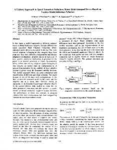
Satellite communications are experiencing very significant technical evolutions, which will be key in defining the role of satellites in future networks as a means to provide broadband access to the Internet over vast coverages. These changes have been enabled by new techniques and technologies: adaptive coding and modulation for the exploitation of EHF bands, where several GHz of bandwidth are available; on board processing for in-space routing; large reflectors for multi-beam antennas with hundreds of spot beams; exploitation of digital beam-forming network concept; as well as significant improvements in on-board power amplification. All of this goes in the direction of maximizing system capacity and flexibility, and in general its effectiveness. On the other hand, satellite broadcasting systems are naturally still focused on the objective of ensuring good coverage over vast areas and, consequently, have hardly exploited the new techniques potential. In fact, the classic Direct to Home (DTH) TV broadcasting satellite network provides service with a single beam typically operated in Ku band, where hundreds of Standard Definition Television (SDTV) or High Definition Television (HDTV) channels can be carried over the entire service area. This is a successful paradigm with seemingly little room for innovation. More recent developments are in the area of Mobile Broadcasting to hand-held terminals, which require a lower frequency band with a more benign propagation environment, such as the S band. Since spectrum availability is here much scarcer (a maximum of 30 MHz), it is necessary to use more efficiently the radio resource by exploiting frequency reuse. Considering European coverage, the satellite antenna pattern is typically organized into country-specific linguistic beams, which are grouped in clusters and assigned different frequency sub-bands, which can be reused in non-adjacent beams. Interference is caused by antenna side-lobes, which must be carefully kept under control. Unfortunately, the amount of reuse that can be achieved is small, and essentially determined by geographic configuration. We propose here a radical increase in the fragmentation of the service area, both for fixed and for mobile applications, through the only exploitation of signal processing techniques over multi-beam antennas with hundreds of beams, also for broadcasting systems. Wherever content is identical in different beams (over a region, a country, or the entire service area) the same frequency band is used to realize a Single Frequency Satellite Network (SFSN), reminiscent of the Single Frequency Network (SFN) concept of terrestrial broadcasting systems, without resorting to any complexity increase in the antenna beamforming or any impact on the receiver. This architecture allows to have unprecedented flexibility in satellite broadcasting systems, as will be discussed shortly. The reason why this idea has never been considered, or it has been rejected altogether, is that the signals carried by multiple beams in a SFSN mutually interfere in overlapping regions, inducing null-capacity zones wherever interference is destructive (see Fig. 12 for an example

17

single frequency satellite networks

of overlapping beams). If no countermeasures are taken, it proves impossible to provide uniform Quality of Service (QoS) throughout the service area. The innovative idea is to use Orthogonal Frequency Division Multiplexing (OFDM) [79] jointly with a new form of MultiBeam Cyclic Delay Diversity (MBCDD) which creates synthetic multipath through the assignment of beam specific power delay profiles. In this way, frequency selectivity is introduced which results in sufficient diversity to avoid destructive interference, guaranteeing correct signal reception in the entire coverage area. Let us dwell briefly over the 400

200

@kmD

18

0

-200

-400 -400

-200

0

@kmD

200

400

Figure 12: 3dB footprint of 400 GEO satellite beams over a 650.000 km2 coverage area. Numerical parameters as in Table 1.

advantages and disadvantages of this approach. As for the main positive aspects, we consider the possibility to: use the same antenna pattern to provide broadcasting and broadband access, for triple play services; deliver efficiently local content and reuse that part of the spectrum extensively; shape precisely and adaptively the contour of beams by grouping spots; use power control selectively over those narrow beams where atmospheric conditions are bad; use a large number of small High Power Amplifiers (HPAs) instead of a few powerful HPAs for the same total power. On the down side, the use of OFDM and MBCDD is not as power efficient as conventional single-carrier techniques, and requires the use of channel equalizers in the receivers. We believe that the advantages largely surpass the negative points. In this chapter, we describe how this idea takes practical form.

2.2 ofdm and cdd

2.2

ofdm and cdd

This section briefly describes the concept of Cyclic Delay Diversity (CDD) for OFDM systems. As well known, OFDM is a multicarrier transmission technique, which splits the available spectrum into several narrowband parallel channels, corresponding to multiple sub-carriers modulated at a low symbol rate. The OFDM signal can be expressed as s(t) =

NFFT ∑−1

t

xk ⋅ ej2πk T ,

(2.1)

−Tg ⩽ t < T

k=0

where xk are the complex-valued modulated data symbols, NFFT is the total number of sub-carriers, T is the useful OFDM symbol time, Tg is the guard interval duration. The guard interval is filled with a cyclic prefix to maintain orthogonality in multipath. Note that, in order to avoid adjacent channel interference, only Na < NFFT active carriers are typically used. Besides using the bandwidth very efficiently, OFDM guarantees high robustness against multipath delay spread, by allowing extremely simple equalization in the frequency domain. So much so that we can increase artificially the channel delay spread by inserting TX-antenna specific cyclic delays. CDD [26], [25] is a Multiple-Input Multiple-Output (MIMO) scheme which allows to enhance the frequency selectivity by inserting additional multiple paths that would not naturally occur. Figure 13 illustrates the block diagram of an OFDM transmitter applying CDD on its NT X antennas. As shown, the same OFDM modu-

CP insertion

CP insertion

OFDM

CP insertion Figure 13: CDD OFDM transmitter.

lated signal is transmitted over NT X antennas with an antenna specific cyclic shift. These shifts are indicated in the time domain by δi , i = 1, ..., NT X − 1, δ ∈ Z and correspond to a multiplication by a phase −j2πf

δi

NFFT factor ψi (f) = e . The latter, together with the normalization term used to split equally the transmission power among the antennas, can be interpreted as due to the channel, leading to an equivalent overall channel transfer function reported in Eq. (2.2) [26]:

1 Heq (f, t) = √ NT X

N∑ T X −1

ψi (f) ⋅ Hi (f, t)

(2.2)

i=0

where Hi (f, t) denotes the channel transfer function from the i-th transmitter antenna to the receiver antenna. Eq. (2.2) applies to the Multiple-

19

20


Input Single-Output (MISO) case, and can obviously be extended to MIMO. Compared to the original propagation channel, the composite channel using CDD shows a much richer multi-path profile, i.e. an increased frequency diversity of the received signal due to the contribution of the CDD transmission scheme. This is especially useful on poor multi-path scenarios in combination with a powerful coding scheme. Here we are interested in the potential of the CDD technique as applied to SFSNs, in association to coded OFDM. Indeed, CDD has been considered for Digital Video Broadcasting Terrestrial (DVB-T) applications [25], but it has never been thought for satellite broadcasting. This is the contribution of the present chapter. 2.3

sfn over satellites

Since the general aim of a broadcast service is to deliver the same signal to a very large audience dislocated over a wide area, one of the most effective solutions is to establish a satellite network. As clearly explained in the Introduction, the main novelty consists in providing broadcasting services through a multi-spot antenna synthesizing local beams, whereby several spots may be sending identical signals, to realize a SFSN. On board multi-beam antennas can be realized through the

Figure 14: Broadcasting over Europe: single beam, linguistic beams, local beams.

adoption of a Cassegrain reflector (which includes a parabolic primary mirror and a hyperbolic secondary mirror) and multi-feed horns; a similar structure to those utilized in Earth station antennas. More precisely, instead of having a single focal point where the feed must be located, the multi-beam antenna has a focal surface on which various feeds can be placed. Such an antenna system has a very compact structure and an adequate flexibility. The design of the reflectors position and feeders configuration realizes the desired beam geometry, in particular the beam overlapping areas on ground and the antenna side-lobes which are the main interference sources. Let us see how a SFSN can be designed exploiting such a multi-beam antenna, through the combined use of OFDM and MBCDD, performing signal processing at the gateway and assuming a transparent satellite transponder with beamforming. 2.3.1

Multi-beam coverage for SFSN

As mentioned before, combining signals coming from two or more overlapping beams generates null-capacity zones wherever they interfere

2.3 sfn over satellites

destructively, causing deep fade events. If fading is frequency nonselective, this means that in certain points of the Earth surface no useful energy can be received. Obviously, this situation would be unacceptable for a broadcasting service since it is impossible to provide a uniform QoS throughout the coverage area. The proposed strategy, relying on the adoption of OFDM on the satellite link, is to apply MBCDD to each beam by imposing a specific delay profile that guarantees frequency selectivity over the signal bandwidth, generating a new source of diversity. This frequency selectivity is beneficial since it can be exploited through coded OFDM and leads to an overall transfer function without any null zone in the entire bandwidth. Consider the k-th beam. Let Hk (f, α, φ) be the channel transfer function corresponding to this beam as seen by a point on Earth reached through a link with amplitude gain α and overall phase rotation φ. Clearly, α accounts for the path loss, while φ includes the initial phase imposed by the gateway transmitter, the phase rotation due to satellite beamforming and that due to propagation delay. Both α and φ are assumed to be constant over the entire signal bandwidth. k Let Hk n = H (n∆f, αk , φk ) be the transfer function coefficient pertaining to the n-th OFDM subcarrier, where the constants αk and φk are implicit for notation simplicity. Assume MBCDD is applied by creating Nk synthetic signal replicas at the gateway, each delayed by δi,k and scaled by an amplitude coefficient Ai,k , for i = 1, . . . , Nk . Thus, the n-th transfer function coefficient can be described as: jφk Hk n (αk , φk ) = αk e

Nk ∑

Ai,k e

−j2πn

mod(δi,k ,NFFT ) NFFT

(2.3)

i=1

where mod(a, b) indicates a module b. The 2Nk + 1 parameters characterizing the power delay profile synthesized for the generic k-th beam give great flexibility, with plenty of degrees of freedom in selecting delays and amplitudes. These parameters can be optimized in the transmitter without any consequences at the receiver. The only constraint is that non selective fading per subcarrier should be guaranteed at all locations, in order to allow simple equalization; besides, channel estimation could became too challenging if the number of paths increases excessively. Note that the application of CDD is not realized with different antennas as in its original form, but through digital processing at the gateway. In this way the system results to be more flexible, since no limitation in the number of delays is introduced, independently of the number of antenna elements. 2.3.2

Spot Beam Radiation Diagram

In order to describe the radiation pattern of each beam, the model described in [78] and [16] has been used. The generic tapered-aperture antenna radiation pattern is reported in the following equation: ( )2 (p + 1)(1 − T ) G(uk ) = GM,k (p + 1)(1 − T ) + T ( )2 2J1 (uk ) T Jp+1 (uk ) p+1 ⋅ +2 p! (2.4) uk 1 − T up+1 k

21

22


where GM,k is the maximum gain for the k-th beam, p is a design parameter, T is the aperture edge taper, Jp (u) is the Bessel function a of the first kind and order p, uk = πd λ sin θk , da,k is the effective antenna aperture for the k-th beam, and λ is the wavelength. Note that in the following, the mask corresponding to G(uk ) with T = 20dB and p = 2, depicted in Fig. 15, has been used. For simplicity, a flat model of the Earth surface has been assumed, which is sufficiently accurate for beams which are not too large and not far from the sub-satellite point. u 5

10

15

20

25

20

-

G[dB] 40

-

60

-

80

-

Figure 15: Spot beam radiation and mask for T = 20dB and p = 2.

2.3.3

MBCDD

Approximated Transfer Function

Now we are in the position to evaluate the overall effect of beam superposition. Let NB be the number of overlapping beams insisting on a specific location with the same transmitted power, and Hn be the overall transfer function coefficient corresponding to the n-th subcarrier. Note that, at any location all αk coefficients are identical for any k; therefore, only φk needs to be explicit. It holds Hn = Hn (φ1 , . . . , φNB ) =

NB ∑ √

G(uk )Hk n (φk )

(2.5)

k=1

The collection of NFFT channel coefficient forms the overall transfer function over the signal bandwidth. Fig. 16 shows a snapshot of this overall transfer function obtained with three overlapping beams having 1, 2, 3, 20 paths at the same power level for NFFT = 2048. Note that, as desired, frequency selectivity is obtained, which enables our SFSN architecture, at the price of the introduction of channel coding and equalization. Since the OFDM signal experiences a frequency selective channel, we need to introduce a figure that can represent the effective performance obtained over the entire band. We elect to use the approximated transfer ¯ defined as the average of the absolute values of the channel function, H, transfer coefficients: ¯ = H

1

N FFT ∑

NFFT

n=1

|Hn |

(2.6)

Note that this function is an approximation of the merit figure shown in the following, which is representative of system performance. Fig. 17 shows the effective transfer function for NB = 3, a fixed value for

2.3 sfn over satellites

5

5

500

1000

1500

2000

500

1000

1500

2000

1500

2000

5

5

-

-

10

-

10

-

15

-

15

-

20

-

(a) N = 1

(b) N = 2 10

5

500

1000

1500

2000

500

5

-

1000

10

-

10

-

20

-

15

-

30

-

20

-

40

-

25

-

(c) N = 3

(d) N = 20

Figure 16: Overall transfer function for three beams and N = 1, 2, 3, 20 paths each beam as a function carrier index.

6

H

4

0

2

10 0 -10 -20 -30 -40 0

Ф2

2

Ф1

4 6

Figure 17: Effective transfer function without MBCDD. Three overlapping beams.

φ3 , and variable φ1 and φ2 . The overlapping beams are assumed to be at the same power level, without MBCDD. Note that for certain combinations of phases the transfer function of the channel without MBCDD presents deep fades of the effective transfer function, which correspond to a null-capacity zone. On the other hand Fig. 18 shows that these fades are resolved with the introduction of MBCDD, even without a specific optimization procedure, that will be described in the following. 2.3.4

Parameter Optimization

The optimized design of the delay profile have not only to avoid signal cancellation for any possible phase shift in the coverage area, but also to minimize the fluctuations of the effective transfer function. The worst case in terms of beam overlap is given by the three beam cluster structure. This means that three typical reception conditions have to be analyzed in order to optimize the provided QoS: one beam, two

23

24


6

4

0

2

10

H 5

0

-5

-10 0

Ф2

2

Ф1

4 6

Figure 18: Effective transfer function with MBCDD. Three overlapping beams. Non-optimized parameters.

overlapping beams, and three overlapping beams. Interference coming from the other beams can be neglected. A deterministic or a statistical design can be followed in order to pursue the optimization. To reduce the number of degrees of freedom, it is possible to assume uniform amplitudes, Ai,k = A ∀ i, k, and equally spaced paths, i.e. δi,k = i ⋅ δ0,k , under the fundamental requirement δ0,1 ∕= δ0,2 ∕= δ0,3 . Moreover, these three parameters can be optimized through the following expression: ( ) ¯ max − H ¯ min δ0,1 , δ0,2 , δ0,3 opt = argmin H (2.7) δ0,1 ,δ0,2 ,δ0,3

where ¯ max = H

max

φ1 ,φ2 ,φ3

( ) ¯ H

¯ min = H

min

φ1 ,φ2 ,φ3

( ) ¯ H

(2.8)

It can be shown that best results are obtained when the following three quantities mod(δ0,1 , NFFT ), mod(δ0,2 , NFFT ), mod(δ0,3 , NFFT ) are incommensurable. Fig. 19 shows an optimized (flat) effective transfer function with incommensurable delays.

6

H

4

0

2

10

5

0

-5

-10 0

Ф2

2

Ф1

4 6

Figure 19: Effective transfer function with MBCDD. Three overlapping beams. Optimized parameters.

2.4 sfsn capacity

2.4

sfsn capacity

In this section we introduce the SFSN capacity in information theoretic terms. Let P/N be the signal-to-noise ratio over a sub-carrier that would be experienced by a receiver in the absence of self-interference generated by CDD and with an isotropic antenna. Thus, in any specific location the capacity can be obtained as [7]: ) ( Na ∑ Fn P (2.9) C= log 1 + N n=1

where Fn = |Hn |2 for MBCDD, while in the case of a single beam Fn only accounts for the antenna gain at the specific location. This function will be used to assess the performance of a SFSN system. Now we will use SFSN capacity shown in Eq. (2.9) to provide an initial comparison between the single and multiple beam cases. In order to ensure fairness, the capacity is estimated assuming to have the same Effective Isotropic Radiated Power (EIRP) available in the two cases. This is reasonable because with multiple beams the antenna gain increases but the beam power decreases. A fair comparison is difficult because the geometry of single-beam/multi-beam coverages are quite different. Let us make a simple assumption which favors completely the single beam case, by placing the user at the sub-satellite point for the single beam case and in the middle point of beam-overlapping regions for the multi-beam case. The capacity obtained in these conditions is shown in Fig. 20. Even in this extreme case, it can be seen that the MBCDD capacity C 6

5

4

3

1 beam 2 overlapping beams 3 overlapping beams

2

5

10

15

20

P/N Figure 20: Capacity comparison in the three scenarios: single beam, two overlapping beams, three overlapping beams.

is not far from the best case of single beam capacity, which is a good and somewhat unexpected result. The comparison would be even more favorable to MBCDD if the average capacity of the entire service area, or the worst case, would be considered. In any case, it is necessary to optimize the on-board antenna radiation diagram (beam apertures and centers) in order to maximize the flatness and fairness of the received power in the entire region.

25

26


2.5

first proof of concept for sfsn

The design of the on-board antenna should be aimed at producing a uniform QoS across the entire service area. We report here a few results obtained in different beam geometry scenarios. The following assumptions have been used: • NFFT = 2048 • Uniform spaced delays, δi = i ⋅ δ0 • Number of multiple paths on each beam Ni equal to 2 • Uniform amplitude delay profile Ai = A within the same beam • Same amplitude delay profile among different beams, A1 = A2 = A3 • Incommensurable delays • Effective antenna aperture da equal to 1.4 m for each beam • Fixed

P N

equal to 7dB

• Service area covered with 6 beams The analysis has been carried out by discretizing the service area into 51 × 51 hexagonal cells and evaluating the capacity in their centers. Moreover, since the capacity behavior is insensitive with respect to the phases φk , as shown in Section 2.3.4 for incommensurable delays, a set of random φk has been chosen for the sake of simplicity. As desired,

C

x y

Figure 21: Capacity obtained in an area covered with six beams.

Fig. 21 shows that a constant capacity can be achieved in the interested area, inside the projected internal circle, where the contributions of the six beams allow an extremely uniform QoS; besides, out of the service region the capacity obviously decreases since there are no

2.6 link budget analysis

beams covering this area. This capacity shaping is clearly detailed also in Fig. 22. The proposed strategy is easily scalable to a wider service area with several beams which provide a very flat capacity all over it.

y

x Figure 22: Snapshot of the capacity obtained in an area covered with six beams.

2.6

link budget analysis

In the following a link budget analysis is shown for the SFSN concept considering, for comparison, also the single beam case with a single carrier transmission and the single beam with OFDM. Note that the analysis has been conducted for a service in Ku band (carrier frequency equal to 12GHz), but the same evaluation can be carried out for other bands. Moreover, a GEO satellite is assumed. All the systems have been dimensioned taking into account the best achievable coverage for an area of 650.000 km2 with the same total transmit power. In particular, for the single beam case, the effective antenna diameter of the satellite has been set to obtain the 3dB edge loss on the border of the coverage area. On the other hand, the effective antenna diameter of each beam in the SFSN has been choose according to the considered beam geometry. In any case, in both the systems, all the parameters in Table 1 have been set in order to have the best trade-off between coverage and link budget requirements. Results in Table 1 show that different signal to noise ratios (P/N) are experienced by a receiver using the three systems. In particular, the use of OFDM both in the SFSN concept and in the single beam requires a larger Output Back Off (OBO) with respect to the single carrier approach. On the other hand, the combining of the signals coming from different beams, foreseen by the SFSN concept, can compensate the losses in the link budget. In the

27

28


Table 1: Link budget for Single Beam and SFSN systems.

Single Beam

OFDM

SFSN

Satellite Tsys

723K

723K

723K

Satellite Antenna Efficiency

0.65

0.65

0.65

Satellite Antenna Diameter

1m

1m

16m

40.11dBi

40.11dBi

64.20dBi

Satellite OBO

1dB

4dB

4dB

Satellite Input Loss

2dB

2dB

2dB

Satellite G/T

11.37dB/K

11.37dB/K

35.45dB/K

Receiver Tsys

150K

150K

150K

Receiver Antenna Efficiency

0.65

0.65

0.65

Receiver Antenna Diameter

0.9m

0.9m

0.9m

39.20dB

39.20dB

39.20dB

17.44dB/K

17.44dB/K

17.44dB/K

3dB

3dB

3dB

Frequency

12GHz

12GHz

12GHz

Bandwidth

500MHz

500MHz

500MHz

Path Loss

205.10dB

205.10dB

205.10dB

1

1

400

19.54dB

19.54dB

−6.48dB

19.54dBW

19.54dBW

19.54dBW

EIRP

53.66dB

50.66dB

48.72dB

P/N

7.60dB

4.60dB

2.67dB

Satellite Antenna Gain

Receiver Antenna Gain Receiver G/T Clear Air Atmospheric Loss

Number of Beams Transmit Power per Beam Total Transmit Power

2.7 numerical evaluation

following section, a more complete comparison of the two systems is conducted, using the signal to noise ratios obtained in this analysis. 2.7

numerical evaluation

Now we calculate the capacity obtained with the single beam scheme and with the SFSN approach. A vast service area of about 650.000 km2 has been considered. Note that this value approximately corresponds to a linguistic beam coverage region. The following assumptions have been used for the SFSN system: • Service area covered with 400 beams organized in a uniform grid (20 × 20) • NFFT = 2048 • Uniform spaced delays, δi = i ⋅ δ0 • Number of multiple paths on each beam Ni equal to 3 • Uniform amplitude delay profile Ai = A within the same beam • Same amplitude delay profile among different beams, A1 = A2 = ... = Ai = ... = A(400) • Incommensurable delays Note that the analysis has been carried out considering the outputs P of Table 1, thus N equal to 7.60dB in the single beam single carrier case, 4.60dB in the single beam with OFDM, and 2.67dB in the SFSN. Moreover, the service area has been discretized into 90 × 90 hexagonal cells and the capacity has been evaluated in their centers. Finally, since the capacity behavior is insensitive with respect to the phases φk , as shown in Section 2.3.4 for incommensurable delays, a set of random φk has been chosen for the sake of simplicity. Fig. 23 shows the capacity comparison between the systems according to the link budget shown in Table 1. As expected, a quasi-constant capacity can be achieved in the interested area, where the contributions of the beams allow an uniform QoS; besides, out of the service region the capacity obviously decreases since there are no beams covering this area. On the other hand, the single beam single carrier approach outperforms SFSN in the zone closer to the center of the coverage area, but results in poorer performance in the zone around the boarder, while the single beam OFDM scheme presents the worst behavior. Note that the proposed strategy is easily scalable also to a smaller or a wider service area, just taking into account the beams position and MBCDD parameters. 2.8

sfsn: pros and cons

Let us dwell over the advantages and disadvantages of this approach. As for the main positive aspects, we consider the possibility to: use the same antenna pattern to provide broadcasting and broadband access, for triple play services; deliver efficiently local content and reuse that part of the spectrum extensively; shape precisely and adaptively the contour of beams by grouping spots; use power control selectively over those narrow beams where atmospheric conditions are bad; use a large number of small HPAs instead of a few powerful HPAs for the same total

29


Single Carrier Single Beam SFSN OFDM Single Beam

2.8 2.6 2.4 Capacity [bit/s/Hz]

30

2.2 2 1.8 1.6 1.4 500 400 300 200 100

0 −100 −200 −300 −400 −500 y [km]

0 −100 −200 −300 −400 −500 x [km]

100

200

300

400

500

Figure 23: Capacity comparison: SFSN vs. Single Beam Single Carrier.

power, reducing thus the non-linear distortion which usually affects satellite systems. Another advantage is related to the complexity, which is confined on the gateway (for the signal processing) and on the satellite (for the increased number of feeders and HPAs) while the receiver design remains unchanged. Furthermore, the only significant issue related to the scalability is the number of beams, while the spectral efficiency is kept constant. On the down side, the use of OFDM and MBCDD is not as power efficient as conventional single-carrier techniques in the center of the beam, and requires the use of channel equalizers in the receivers. However, this is not a relevant problem, since the equalization is performed in the frequency domain and even a single carrier receivers shall provide at least an Automatic Gain Control (AGC) device in order to have channel equalization. 2.9

conclusions

This chapter contains a novel approach for multi-spot broadcasting systems via satellite. Relying on the SFN concept and OFDM principles, uniform coverage and QoS can be guaranteed by applying the CDD technique on each beam to eliminate the null-capacity zones by introducing frequency selectivity. A link budget analysis is proposed in order to perform a fair comparison between SFSN and a classical single beam single carrier system. As expected, differently from the single beam, the SFSN system is able to guarantee a flat capacity over the entire service area, at the cost of a correct design of beams position and CDD parameters. However, this design is computed once for all, and involves only the gateway for signal processing and the satellite for beam shaping. No further complexity is required at the receiver. An operator adopting

2.9 conclusions

the concept of SFSN will enjoy unprecedented broadcasting flexibility and ease of convergence with broadband services.

31

𝟑

Q U A S I - C O N S TA N T E N V E L O P E O F D M

3.1

introduction

Orthogonal Frequency Division Multiplexing (OFDM) modulation has raised to a de-facto standard in modern wireless communication. This flexible modulation scheme can be efficiently used over frequency selective channels, with effective equalization. One of the drawbacks of OFDM systems, hovewer, is the resilience to non linear distortion, which is considerably inferior to single carrier system. This is due to the envelope fluctuation of the OFDM-modulated signal, which, by a Central Limit Theorem may be approximated by a Gaussian variable. Several studies have been performed about the impact of non-linearities on Gaussian signals, in particular [15] and [57] gave the basis to analyze the behavior of OFDM system in presence of non linearities. Bussgang [15] stated that the output of a non linear system fed by Gaussian signal can be expressed as a scaled replica of the input and a noise uncorrelated to the input. Minkoff [57] extended this work to complex signal, highlighting the so-called AM-PM conversion that is the phase distortion in output signal. Based on these early studies on Gaussian signals, when OFDM started to be applied, its performance on non-linear channels were analyzed, and the large loss in performance due to the distortion can be seen in [5, 4], where the analysis is carried out for Additive White Gaussian Noise (AWGN) and fading channels, respectively. As it can be clearly seen in these reference, the loss from AWGN channels to non-linear channel is considerable, and prevented, for the first period, to apply OFDM modulation on severely degraded channels such as the Land-Mobile-Satellite channel. Two approaches were considered against non linear distortion: predistortion and Peak-to-Average-Power Ratio (PAPR) reduction. The first one is more traditional, can be applied even to single carrier systems and consist in providing a predistorter [67], i.e. a block before the High Power Amplifier (HPA) whose aim is to invert the HPA transfer function. In other words, the cascade of predistorter and HPA should be a linear amplifier, at least in the signal dynamic range. This approach is commonly adopted, and its performances are quite interesting if the amplifier is conveniently driven far from its saturation point (an Input Back Off (IBO) of 1 to 3 dB is required for single carrier transmission, while for multicarrier the back off should increase). The second approach is more specific of OFDM system, and consists in reducing the fluctuations of the envelope of the signal. In this way, the transmitted signal should not be damaged too much by the non linear distortion. These techniques, described in [40, 48], can operate in different ways: some technique provide alternative representation of the signal, and make a side information available at the receiver. Other techniques perform operations in order to cancel the peak, using some reserved carriers or modifying the points on their initial constellations. Other techniques are related to coding schemes or to non linear processing on the signal (exponential companding and similars). The main drawback of these family of techniques is the reduction in throughput, or the

33

34

quasi-constant envelope ofdm

complexity increase they cause. Using the pervious mentioned methods the PAPR can be kept moderately low, with a reduction of several dB with respect to the original signal. However this PAPR reduction could be not sufficient to guarantee a satisfying OFDM reception in presence of a severe non-linear channel. Our purpose is to obtain a dramatic PAPR reduction, which yields to an OFDM signals having a quasi-constant envelope, in order to make OFDM reception feasible even in those scenarios characterized by severe non-linearities. In particular, we target to keep the PAPR around 1 − 2 dB which corresponds to a reduction of almost ten dB with respect to the original signal. In order to achieve such a ambitious purpose we introduce a novel PAPR technique based on a open data mapping which, by exploiting some of its degree of freedom and using an optimization process can guarantee a quasi-constant envelope. There is a straightforward trade off between the amount of flexibility that the open data mapping exploits to reduce the PAPR and the its robustness to gaussian noise, as well as its spectral efficiency. For this reason we also propose some different kind of open data mappings that represents different compromises between PAPR reduction and Gaussian noise robustness. 3.2 3.2.1

context system model Nonlinear Distortion

We address the distortion owing to HPA, which acts on both the envelope (AM/AM) and phase (AM/PM) of the OFDM signal. Considering a generic complex nonlinear distortion function the output signal can be expressed as: sd (t) = F[ρ(t)]e{

∕ s(t)+Φ[ρ(t)]}

(3.1)

Where ρ(t) and ∕ s(t) represent respectively the envelope and the phase of s(t), and F[⋅] and Φ[⋅] represent respectively the AM/AM and AM/PM characteristics. Note that the nonlinear distortion function only depends on the envelope of the input signal. In its original writing Bussgang Theorem states: “For two gaussian signals, the cross-correlation function taken after one of them has undergone nonlinear amplitude distortion is identical, except for a factor of proportionality, to the cross-correlation function taken before the distortion.” The mathematical expression of this stated theorem is as follows: < y(t)s∗d (t) >= α < y(t)s∗ (t) > where

(3.2)

∫ T/2

= lim 1/T T →∞

a(t) dt

(3.3)

−T/2

and y(t) and s(t) are gaussian random process. In the particular case of y(t) = x(t + τ): < s(t + τ)s∗d (t) >= α < s(t + τ)s∗ (t) > ∀τ

(3.4)

The Bussgang theorem gives us the proof of the separability of a non linear output as the sum of a useful attenuated input replica and an uncorrelated nonlinear distortion, thus we can write the output as: sd (t) = αs(t) + d(t)

(3.5)

3.2 context system model

where < s(t + τ)d(t) >= 0 ∀τ

(3.6)

and the complex attenuation coefficient α is given by: α=

< s(t)s∗d (t) > < s(t)s∗ (t) >

Assuming the ergodicity of s(t), (3.7) can be expressed as: (∫ ∞ )∗ 1 −Φ[ρ(t)] F[ρ(t)]e ρ(t) p(ρ) dρ α= 2 σ 0

(3.7)

(3.8)

where σ2 represent the power of s(t), p(ρ) is the Rayleigh probability density function, which characterizes ρ(t), the envelope of s(t), and the conjugates make sense if and only if the nonlinear function has complex values. Following the tractation in [80], it can be useful to define a scaling parameter β such as E[s2d ] = βE[s2 ] = |α|2 E[s2 ] + E[d2 ] and it can be written as ∫∞ 1 β= |F[ρ(t)]|2 p(ρ)dρ E[s2 ] 0

(3.9)

(3.10)

In this way, the power of the useful signal and the distortion noise are |α|2 and (β − |α|2 ) respectively The IBO is an important system parameter useful to describe the operating power of the amplifier. It is defined as the ratio between the input saturation power and the actual input average power. Similarly, the Output Back Off (OBO) is defined as the ratio between the output saturation power and the output average power. In formulas IBO = OBO

=

sat Pin [ ] E |s|2

(3.11)

sat Pout ] [ E |sd |2

(3.12)

Now we considerer a simple Ideal Clipping (IC) Nonlinear Distortion, also known as Soft Limiter, which is the memoryless model corresponding to the ideal case of perfect predistortion. In other words we assume that the predistortion is able to perfectly compensate the non-linearities due to the HPA up to the saturation point. In this case we have a linear transfer function before the saturation zone and an ideal clipping inside the saturation zone, thus its AM/AM and AM/PM characteristics are given respectively by:  ρ if ρ ⩽ A F(ρ) = (3.13)  A if ρ > A

Φ(ρ) = 0

(3.14)

35

36


where A is the saturation amplitude. This model has a normalized gain, which is set to 1 without loss of generality. From (3.8) the coefficient α is given by [27, 62]: √ ( ) 2 πA2 /σ2 A − A2 (3.15) α = 1−e σ + erfc 2 σ Similarly, for β we have 2

− A2

β = 1−e

(3.16)

σ

Saleh model [66] is a common model for Travelling Wave Tube Amplifiers (TWTA), obtained through best-fit of sperimental data. While it may fit every TWTA, a particular choice of its parameters was widely used in analytical studies, leading to the AM/AM and AM/PM characteristics reported below F(ρ)

=

Φ(ρ)

=

2ρ 1 + ρ2 π ρ2 6 1 + ρ2

(3.17) (3.18)

This model was normalized in order to have the saturation point in ρ = 1. For this reason the input power is supposed to be less than 1 if the amplifier is driven in a fairly nonlinear region of its characteristic. The calculation of the parameters α and β is very difficult for this model. While a closed form expression can be difficult to evaluate, involving special functions such as the exponential integral function, while numerical integration formulas easily led to the following results back off [dB]

α

β

0

0.7737 + 0.2172

0.7708

0.5

0.8233 + 0.2213

0.8538

1

0.8738 + 0.2245

0.942

2

0.9767 + 0.2277

1.133

3

1.081 + 0.2266

1.342

4

1.183 + 0.2212

1.563

5

1.283 + 0.2118

1.793

6

1.377 + 0.1989

2.026

Table 2: Values of α and β for the Saleh model.

The values of β greater than one can be explained observing the expression of the AM/AM characteristic in Eq. (3.17): if the amplifier is driven in its linear region (i.e. for lower values of r), the power gain of the amplifier is 4, while if the amplifier is driven near to the saturation, the gain obviously decreases. 3.2.2

OFDM

signal

We consider an OFDM signal with N total subcarriers and Na , Na < N, active subcarriers1 . The ℓ-th OFDM symbol, s¯ ℓ = (s0,ℓ , . . . , sN−1,ℓ ), is 1 The number of active subcarriers, Na , is chosen so as to respect the spectrum mask, i.e., to introduce guard bands at the edges of the used spectrum band.

3.2 context system model

obtained as the N points Inverse Discrete Fourier Transform (IDFT) of the vector of complex symbols x¯ ℓ = (x0,ℓ , . . . , xN−1,ℓ ), as N−1 1 ∑ si,ℓ = √ xk,ℓ e 2πki/N N k=0

i = 0, . . . , N − 1

(3.19)

a where xk,ℓ = 0 if k < NB or k > N − NB , being NB = ⌊ N−N ⌋ the 2 number of subcarriers in the guardbands. In order to avoid intersymbol interference and maintain subcarrier orthogonality even in multipath, a cyclic prefix of length Ng samples is inserted at the beginning of each OFDM symbol. This is followed by digital to analogue conversion at sampling rate R = 1/T , so that the time continuous signal can be written as

( ) N−1 ∞ ∑ ∑ 1 1 t 1 s(t) = √ rect − −ℓ xk,ℓ e 2π Tu k(t−Tg ) (3.20) TL 2 Tu ℓ=−∞ k=0 where Tu = NT represents the OFDM useful symbol duration, Tg = Ng T represents the duration of the guard interval associated to the cyclic prefix, therefore TL = Tu + Tg is the total OFDM symbol duration, and fu = 1/Tu is the subcarrier spacing. If N is sufficiently large, the signal s(t) expressed in (3.20) can be considered as a Gaussian complex random process as a consequence of the central limit theorem. Bussgang’s theorem guarantees that the signal sd after the nonlinear distortion, can be split in two terms: a linear term that is proportional to s(t) according to a constant α, and a nonlinear distortion term, d(t), that is a zero-mean (not Gaussian) process uncorrelated from s(t): sd (t) = αs(t) + d(t)

(3.21)

In this case it is interesting to define a merit figure, the Signal-toDistortion Ratio (SDR), which describes the impact of signal scaling and additive distortion noise. Assuming E[|s(t)|2 ] = 1 we have: . SDR =

|α|2 E[|d(t)|2 ]

(3.22)

The OFDM signal, sd (t) is transmitted over a time-varying frequency selective fading channel, under the assumption that the channel coherence time exceeds TL . The baseband equivalent channel impulse response is modeled as a tapped delay line: h(t) =

N∑ m −1

( ) hj (t)δ t − τj (t)

(3.23)

j=0

where hj (t) and τj are respectively the gain and delay of the j-th path, and Nm represents the number of multiple propagation paths. In Rayleigh fading, at any time instant hj (t) can be modeled as a complex Gaussian random variable with zero mean and variance γ2j /2 per ∑ branch. The total channel energy is normalized to one, i.e. j E[h2j ] = ∑ 2 j γj = 1, and the maximum delay is assumed to be smaller than the guard interval duration, i. e. τmax = maxj τj < Tg . The received signal can be written as r(t) = h(t) ∗ (αs(t) + d(t)) + n(t)

(3.24)

37

38


where n(t) represents a Complex AWGN random process, with twosided power spectral density equal to N0 . Filtering and sampling the received signal every T seconds yields ∑ r(uT ) = hj (uT ) ⋅ αs(uT − τj ) + d(uT − τj ) + n(uT ) (3.25) j

Removing the guard interval and re-arranging the vector at the input of the Fast Fourier Transform (FFT), the samples belonging to the ℓ-th OFDM symbols can be collected into a vector r¯ ℓ with components: ri,ℓ = r(((ℓ − 1)(N + Ng ) + Ng + i)T ) i = |u|N+Ng − Ng

ℓ = ⌈u/(N + Ng )⌉

(3.26)

Assuming that hj (t) remains constant over a OFDM symbol duration, at the output of the FFT, in the frequency domain, the OFDM symbol is: yk,ℓ

=

N−1 1 ∑ √ ri,ℓ ⋅ e− 2πki/N N i=0

= Hk,ℓ (αxk,ℓ + Dk,ℓ ) + nk,ℓ

(3.27) k = 0, . . . , N − 1

(3.28)

where according with (3.19) Discrete Fourier Transform (DFT) normalization factor √1 has been taken into account, nk,ℓ is the complex N AWGN sample in frequency domain, and Hk,ℓ is the at the subcarrier k, in the ℓ-th symbol: N−1 1 ∑ Hk,ℓ = √ hj e− 2πkτj /Tu N j=0

3.3 3.3.1

(3.29)

rotation-invariant subcarrier mapping Constellation design

We introduce a novel concept for subcarriers data mapping where the symbols belonging to the modulation alphabet are not anchored, but they maintain some degree of freedom, for this reason we refer to it as open data mapping. The final positions of the transmitted complex symbols are chosen by an iterative optimization process that arranges them in order to decrease the resulting OFDM symbol PAPR. The first open mapping scheme we propose is a very easy two-order data mapping, illustrated in figure 24, where the bit ’0’ is mapped in zero and the bit ’1’ can be mapped in any points of the belonging to √ the circle with radius 2Eb and centered in zero. In formulas, the data mapping is  0 if bk = 0 xk = √ (3.30)  2Eb eφk if bk = 1 where bk is the k-th bit to be mapped, and the values of φk will be optimized according to the algorithm described in following. 3.3.2

Spherical Active Constellation Extension (ACE)

This algorithm arranges the phases φk in order to decrease the resulting OFDM symbol PAPR. It works alternating time and frequency domain,

3.3 rotation-invariant subcarrier mapping

1.5

1

0.5

0

−0.5

−1

−1.5 −1.5

−1

−0.5

0

0.5

1

1.5

Figure 24: Circularly simmetrical constellation.

and its parameters are the number of iteration Niter , and the threshold, ξ, used in clipping the signal. This iterative algorithm works alternately in time and frequency domain as follows: • First, the time domain samples si whose absolute value exceeds the threshold ξ are clipped. • Then, passing to frequency domain, the complex data xk are reinstated at the zero or on the circumference modifying only their absolute values. In this manner the constellation constraints are restored. • Subsequently, in the time domain, the samples si are clipped again, then the constellation constraints are restored. These operation are repeated Niter times. This procedure converges, because it can be seen as a projection onto a convex set, and it will converge to a signal with the lowest possible PAPR. This algorithm is an original extension of the ACE method used in traditional PAPR reduction techniques [52]. The main difference is that the Spherical ACE move the complex data xk only acting on their phase. In this way the energy of each complex data xk remains constant, and the distance among the points of constellation in equal. 3.3.3

Extensions

Some further extension of this approach are possible, in order to increase the spectral efficiency or the resilience to the AWGN. For instance,

39

40


a straightforward extension of the aforementioned technique requires the origin and three rings to map two information bits. Another open mapping scheme which provides spectral efficiency of 2 bit/channel and ensures an increased distance between points, is the so-called clover mapping, depicted in figure 25. Unfortunately in this case Graymapping is not applicable. In formulas, the data mapping is described

1.5

1

0.5

0

−0.5

−1

−1.5 −1.5

−1

−0.5

0

0.5

1

1.5

Figure 25: Clover constellation.

by Eq. (3.31)    0   √    4 φk  , 3 Es xk = √  4 φk ,   3 Es   √    4 Es φk , 3 3.4

if bk = 00 [ ] π φk ∈ − π 6 , 6 if bk = 01 [ 5π ] φk ∈ 𝒰 π 2 , 6 if bk = 10 [ 5π π ] φk ∈ 𝒰 − 6 , 2 if bk = 11

(3.31)

awgn detectors

In this section, first we propose the detection scheme for our open data mappings, and secondly we analyze the performance of the proposed mapping schemes. The analytical assesment hereby presented is based on a simple AWGN channel. This is convenient for analytical simplicity and does not affect the generality of the discussion, since the effect of the HPA distortion can be modeled as a scaling of the useful signal and an additional noise source. Under these assumptions equation (3.27) becomes yk,l = xk,l + nk,l

(3.32)

3.5 numerical results

where nk,y ∼ 𝒩(0, N0 /2) represents the AWGN term. For the first mapping scheme presented in Section 3.3.1 and described by equation (3.30) the envelope of the received signal can be modeled as a Rayleigh random variable if bk = 0 and a Rice r.v. if bk = 1. Letting ρy be the envelope of the received signal, we have  2ρ2 y   2ρy − N0 if bk = 0 pρy (ρy ) = N0 ρ2y +2E (3.33) ) ( √ b   2ρy − N0 I 2ρy 2Eb if b = 1 k 0 N0 N0 where we have dropped the subscript l, for the sake of readability. The energy detector can be efficiently employed for this problem: the randomness of the phase due to spherical ACE inhibits the use of a coherent detector, and the energy detector is both robust and simple. The threshold ξ on the received signal can thus be calculated by the Maximum Likelihood (ML) criterion (equal symbol a priori probability and equal cost of the errors), leading to the following non linear equation pρy |bk =1 (ξ|bk = 1) = pρy |bk =0 (ξ|bk = 0)

(3.34)

whose solution can be found numerically. Once the value for the threshold ξ is obtained, the error probability can be written as ∫ ∫ 1 ξ 1 ∞ Pe = pρy |bk =1 (ρk |bk = 1)dρk + p (ρk |bk = 0)dρk 2 0 2 ξ ρy |bk =0 √ ( √ [ )] 1 − N2ξ 1 Eb 2 = e 0 + 1 − Q1 2 ,ξ (3.35) 2 2 N0 N0 where Q1 (a, b) is the Marcum-Q function [1]. In the case of a transmission impaired by a distorting HPA, the noise term must include also the effect of the HPA (the term Dk,l ) in equation 3.27 The performances of the proposed detector are shown in figure 26 The Clover constellation detection problem is analytically involved, since it would require a perfect knowledge of the phase distribution after the Spherical ACE routine. This knowledge will be necessary to define the likelihood functions related to the four different symbol hypotheses. Since the phase distribution is almost impossible to determine in an analytical fashion, and it depends strongly on the clipping thresholds, we preferred to employ an sub-optimal detector, rather than to postulate a model for the phase distribution. In our approximate model the detection is performed in two steps: in the first the central symbol is separated out of the 3 symbols lying on the external ring. In this stage an energy detector is again employed, but it has a different threshold with respect to the case of the Saturn Modulation, due to difference in both signal amplitude and probability of the outer ring. Once this first detection has been performed, in case the signal is supposed to belong to the outer ring, a phase detector is employed. Summarizing, figure 27 reports the decision regions, while figure 28 shows the performance of this sub-optimal detector on the AWGN channel 3.5

numerical results

The first result in Fig. 29 we present is the Complementary Cumulative Density Function (CCDF) of the PAPR distribution for the modulation

41


0

10

−1

10

Pe

42

−2

10

−3

10

0

2

4

6

8

10

Es/N0 [dB]

Figure 26: Error Probability of Two Level Mapping.

2 1.5 1 0.5 0 −0.5 −1 −1.5 −2 −2

−1

0

1

Figure 27: Decision Regions for Clover Mapping.

2

3.5 numerical results

0

10

−1

Pb

10

−2

10

−3

10

−4

10

0

2

4

6

8

10

Eb/N0 [dB]

Figure 28: Bit Error Probability for Clover Mapping.

scheme introduced in the previous sections. Although the PAPR reduction offered by ACE is surely significant, our proposed mappings can achieve a quasi constant envelope, resulting in a very low PAPR. 1.E+00 Two level modulation Clover ACE-QPSK

1.E-01

QPSK C C 1.E-02 D F

1.E-03

1.E-04 0

1

2

3

4

5

6

7

8

9

10

11

12

13

14

15

PAPR [dB]

Figure 29: PAPR distribution for Two level and Clover Mappings.

The impact of such a low PAPR is highlighted by Fig. 30,31: our proposed schemes achieve the best performances in terms of SDR over a strongly non-linear channel (the IBO for both Saleh and IC HPAs is lower than 1) Finally, Fig. 32,33 show the impact in terms of Bit Error Rate (BER) of the excellent PAPR reduction achieved by our proposals. As the figures show, the PAPR reduction does not directly translate into a BER improvement. However, our scheme allow to communicate reliably over

43


SDR [dB]

20

10

Two Level Modulation Clover ACE-QPSK QPSK 0 0.3

0.5

0.7

1

IBO [dB]

Figure 30: SDR on Saleh HPA vs IBO for the proposed mappings.

70

Two Level Modulation Clover 60

ACE-QPSK QPSK

50

SDR [dB]

44

40

30

20

10 0.3

0.5

0.7

1

IBO [dB]

Figure 31: SDR on IC HPA vs IBO for the proposed mappings.

3.6 conclusions

a strongly non-linear channel,such as a Saleh HPA with an IBO equal to 0 dB. QPSK ACE-QPSK Clover Two level modulation

BER

Eb/N0 [dB]

Figure 32: BER on Saleh HPA at IBO = 0 dB for the proposed mappings.

!#"!%$'&(*)*+,$ - .0/ 21 3 $ "!%4 56367 8:9

9

Eb/N0 [dB]

Figure 33: BER on IC HPA at IBO = 0 dB for the proposed mappings.

3.6

conclusions

This chapter presented a novel concept for data mapping. Using rotationally invariant sub-carrier mapping we are able to reduce dramatically the PAPR, allowing thus to receive reliably over strongly non-linear channels. Our approach is based on a iterative optimization routine, which is an original broadening of the ACE method [52]. The innovation we proposed is in the active role of the symbol phases to effectively reduce the PAPR.

45

𝟒

F U RT H E R D E V E L O P M E N T S O F T H E P R E S E N T E D WORK

There are various possible developments for the work presented in this thesis. This final chapter recollects some of the future directions in which the research in the field of Physical Layer (PHY) optimization for Orthogonal Frequency Division Multiplexing (OFDM) systems will continue. Multicarrier modulation, although already adopted in various transmission standards, has further room for improvements. First of all, the optimization of payload and pilots is an interesting area, now dominated by “rules of thumb” or “separate boxes” optimization of all receiving circuits. Secondly, the next years will see the adoption of multicarrier modulations in almost all possible scenarios. Therefore new methods are to be found to enhance the resilience of this waveform, or to increase the spectral efficiency. In this future scenario, the efforts on Single Frequency Satellite Networks and on Quasi-constant Envelope OFDM will be surely continued. For the first case, i. e. Single Frequency Satellite Network (SFSN), the reuse of mobile satellite services bands is indeed a real problem, and the adoption of a SFSN would be of great utility. At any rate, the next possible study on SFSN should be an end-to-end simulation, including channel estimation and synchronization issues. We expect to see an obvious performance loss with respect to the ideal case, however we believe that the advantages of SFSN will be fully confirmed. The resilience of OFDM to non-linearities is another topic that needs further investigations: the present approach to cope with this problem is to use more robust subcarrier mappings (i. e. Quaternary Phase Shift Keying (QPSK) rather than high order Quadrature Amplitude Modulation (QAM)) and to reduce the code rate. On the contrary, we believe that the OFDM waveform can be modified and improved, in order to achieve a more than satisfactory trade off between the reduction of the signal dynamics (and thus the increase of the signal robustness to non-linearities) and the Quality of Service (QoS) at the receiver. Summarizing, the world is still going wireless, and the PHY research is not dead, notwithstanding all the catastrophic announcements on this regard which were given in the last decades. The extension of wideband signal to very harsh scenarios offers a lot of challenges, which will be accepted and solved by a mixture of creativity and technical knowledge.

47

Part II I N N O VAT I O N S I N S I N G L E C A R R I E R SYSTEMS

𝟓

O P T I M I Z AT I O N O F C O N S T E L L AT I O N S O V E R NON-LINEAR CHANNELS

5.1

introduction

The non-linear satellite channel has been extensively studied in the literature, mainly through numerical evaluation, at least for those cases in which the High Power Amplifier (HPA) characteristics are only given empirically. However, analytical approaches to the optimization of signal constellations appear to be an interesting problem that needs to be addressed and can in fact be exploited in system design and air-interface definition. In this chapter we will introduce an analytical approach for the optimization of signal constellations for the satellite channel, or more generally, for a noisy and non-linear channel, under the constraint of normalized constellation energy. Among all of the possible definitions of optimality, we consider the minimum average error probability criterion, that is, the optimal constellation leads to the minimum mean error probability under the assumption of using a maximum likelihood detector. As a consequence, the optimal constellation is the one which, for a given transmitted power, maximizes the mutual distance amongst constellation points. Let {si }, i = 1 . . . M

(5.1)

be the constellation points, where si ∈ C and M is the constellation cardinality, and let the constellation be normalized to unit average energy, i.e. M 1 ∑ 2 |si | = 1 M

(5.2)

i=1

The problem consists in finding optimal positions for the points. Foschini et al. in [35] proved that in a Additive White Gaussian Noise (AWGN) channel the optimal signal constellation, for increasing cardinality, tends to a triangular lattice, and showed that the optimum 16-point constellation gains 0.5dB in Signal-to-Noise Ratio (SNR) with respect to 16-Quadrature Amplitude Modulation (QAM). The problem of finding the optimal signal set was handled also by Kearson [39, 50], who released the assumption of Gaussian noise, finding the optimal signal constellation for various noise distributions. Due to the presence of non-linear distortion the above results cannot be readily applied to the satellite channel. The effect of non-linear amplification on signal transmission are various: first of all, a rotation of the whole signal set is observed (AM-PM conversion). Constellation points are also more near each other, due to the saturation in the amplifier (warping). Lastly, clustering phenomenon appears, which consists of receiving a cluster of points instead of a single constellation point. This is due to non-linear processing of transmitted pulses and to the consequent violation of Nyquist condition for Inter-Symbol Interference (ISI) avoidance at the receiver.

51

52

optimization of constellations over non-linear channels

There are various approach to model the satellite channel with distorting amplifier. A complete and analytic tool is given by Volterra series (see [9] or [10] for an example of application). The Saleh model [66] allows to determine analitically the constellation rotation and warping, while the evaluation of clustering must be performed through computer simulations. The approach used in [60] and [61], that is to consider the channel free from ISI, could be difficult to adapt in typical satellite transmission, considering the importance of filtering in order to reduce Adjacent Channel Interference (ACI). Our method follows a more realistic approach: the constellation rotation and warping is modeled according to Saleh [66], while the clustering is modeled as another additive white Gaussian noise. This simplified approach can be theoretically justified by Central Limit Theorem if the duration of transmitted pulse is significantly longer than symbol time, and has the advantage of requiring less simulation time and allowing to use formulas for error probability in AWGN, with the necessary corrections due to the warping. The exact calculation of the error probability for complex signal constellations is still an open problem. It can be solved numerically, for example by the technique of decomposing decision region proposed in [24] or in [74], but a closed form solution, for a general constellation, is lacking. Various upper and lower bounds have been proposed in the last decades. The Union Bound is the simpler version of the Bonferroni inequality ([22, Chap. 2]) approach, and becames increasingly tighter for increasing SNR. High order Bonferroni inequalities are too computationally expensive, so other approaches have been preferred: Seguin [69], Kuai et al. [54] have proposed new forms of lower bounds, Poscetti [65], Hughes [44] and Swaszech [73] have proposed upper or lower bound based on a geometrical approach, but such a method is not suitable for analytic optimization. Thus the Union Bound is a good candidate for calculating error probability, because it is a good compromise between complexity and accuracy, for its analytical origin, and for the fact that an upper bound is a more conservative approach to our problem, and in general to communication systems design. Summarizing, we aim at finding the constellations which yield the best performance over a noisy and nonlinear channel, and the method we propose is to optimize the constellation point positions by a gradient method, using as objective function the expression of symbol error probability given by the Union Bound The rest of this chapter is structured as follows: Section 5.2 presents the system model and the probability of error for such a system. Section 5.3 describes the used algorithm and discusses its performance. Results are shown in Section 5.4 and the conclusion are presented in Section 5.5 5.2 5.2.1

system model Received Signal

We consider a simplified two-dimensional M-ary synchronous data transmission, in which the message, mapped in a symbol from the constellation in Eq. (6.1), say the i-th, is processed by a pulse-shaping filter and a non-linear amplifier, is then transmitted through an AWGN channel, and, at the receiver, it undergoes matched filtering and sampling. Assuming ideal recovery of carrier phase and frequency, and of

5.2 system model

timing offset, the expression of the signal which is fed to the decision device at the k−th symbol time is √ rk = Es ⋅ ci,k + µk + νk (5.3) where µk = µp,k + jµq,k , µp,k , µq,k ∼ 𝒩(0,

NA ) 2

(5.4)

is the noise due to nonlinear pulse processing, whose variance NA can be obtained experimentally, or via the method indicated in [9], and νk = νp,k + jνq,k , νp,k , νq,k ∼ 𝒩(0,

N0 ) 2

(5.5)

is the AWGN term having variance N0 /2 per component. Both Gaussian processes are supposed to be white, and, for the interference contibution, we will omit its dependence from the constellation symbols, assuming thus a worst-case approach. Finally, ci is a point of the distorted constellation, whose value can be obtained from the original signal point si , characterizing the amplifier with the Saleh model [66] 1 ci = √∑ M

j=1 |sj,d

where

|2

si,d eφi,d

si,d

=

√ 2 β|si | 1 + β|si |2

φi,d

=

π β|si |2 3 1 + β|si |2

(5.6)

(5.7) (5.8)

and β is the Input Back Off (IBO), an indication about how far the amplifier is driven off saturation. 5.2.2

Error Probability

In this section we will determine the average symbol error probability, assuming equiprobable signalling, and using the Union Bound, for the ease of analytical tractability. The average symbol error probability can be written as: Pe =

M 1 ∑ Pe (si ) M

(5.9)

i=1

where the last term is the conditional probability of error when symbol si is transmitted, and can be upper bounded by: Pe (si ) ⩽

M ∑

( ) Prob sˆ j |si

(5.10)

j=1 j∕=i

( ) The last term, Prob sˆ j |si , the probability of deciding for sj when si was transmitted, can be expressed as

) ( √ √ ( )

Prob sˆ j |si = Prob r − Es cj ⩽ r − Es ci (5.11)

53

54


where we have assumed that the receiver knows the distorted constellation and the carrier phase was ideally recovered. Recalling the properties of Gaussian variables, the expression for the error probability is (

) M M √ cj − ci 1 ∑∑ 1 Pe ⩽ erfc γ (5.12) M 2 2 i=1 j=1 j∕=i

where γ = 5.3 5.3.1

Es NA +N0 .

proposed algorithm Description

The upper bound for the error probability written above, which depends on the signal constellation, can be used as the objective function in a constrained optimization problem. Solving the constrained optimization problem via an iterative gradient method yields the optimal constellation point displacement, constrained to have unit average energy The algorithm used to optimize constellation is composed of the following steps: 1. Non-linear distortion application, obtaining {si,d eφi,d }, 1...M

i =

2. Normalization of constellation, obtaining {ci } i = 1 . . . M 3. Calculation of ∇Pe : [∇Pe ]k =

∂Pe ∂ck

4. Constellation update: sk = sk − α [∇Pe ]k 5. Constellation normalization {si }, i = 1 . . . M 6. Apply stopping rule or iterate The stopping rule could be the reaching of a maximum number of iterations, or the convergence of the solution (i.e. the constellations between two consecutive iteration differ for a given small value) The output of this procedure is the constellation that, on a noisy non-linear channel yields the lowest error probability. That is, the constellation that after the distortion preserves the distance between points. The critical step which requires detailed mathematical consideration is the calculation of ∇Pe for the distorted constellation {ci }. Considering the i−th component of the gradient, we have: [∇Pe ]i

=

∂Pe ∂ci

=

) M √ cj − ci 1 ∑ ∂ erfc γ = M ∂ci 2

(5.13) (

(5.14)

j=1 j∕=i

=

2 √ M ] γ [ 1 ∑ 2 − γ∥cj −ci ∥ 4 √ e 1 cj − ci M 2 π

(5.15)

j=1 j∕=i

where 1(cj − ci ) is a unit vector applied in ci and making an angle { } with the x-axis equal to arg cj − ci .

5.3 proposed algorithm

5.3.2

Convergence

The convergence of the algorithm can be assured using a result found in [12], if the function, say F(x), to be minimized over the domain 𝒟 satisfies the Lipschitz condition ∥∇F(x) − ∇F(y)∥2 ⩽ K ∥x − y∥2 ,

∀x, y ∈ 𝒟

(5.16)

2 and the step α in the gradient method is chosen to satisfy 0 ⩽ α ⩽ K . In this case, the fulfillment of the Lipschitz condition and the value of the parameter K follow from the Mean Value Theorem for vector functions:

∇F(x) − ∇F(y) = H(z)(x − y)

(5.17)

where z ∈ 𝒟, and H(⋅) is the Hessian matrix, defined as hij = Moreover, [

∥∇F(x) − ∇F(y)∥2

]

∂2 F ∂xi ∂xj .

⩽ ∥H(z)∥2 ∥x − y∥2 ⩽ ∥H(z)∥F ∥x − y∥2

(5.18)

where ∥H∥F is the Frobenius (or Hilbert-Schmidt) norm, defined as v u Nr Nc u∑ ∑ ∥H∥F = ⎷ |hij |2 (5.19) i=1 j=1

where Nr and Nc are, respectively, the number of rows and columns of H. Thus, setting K as K = max ∥H(z)∥F z∈𝒟

(5.20)

assures the satisfaction of the Lipschitz condition in Eq. (5.16) In our case, the calculation of the Hessian matrix of the error probability function is easy due to the exponential nature of the function, and releasing the unit average energy constraint for signal points, a loose bound on the algorithm step can be obtained with some algebraic manipulations. After having assumed the negative exponentials equal to 1, we have |hij |2 ⩽

γ3 ∥cj − ci ∥2 4πM2

(5.21)

the last factor, i. e. ∥cj − ci ∥2 depends of course from the two points ci and cj . At any rate, considering the placements of the point in one or more rings to cope with the non-linear distortion due to the HPA, it is very unlikely to see constellation points having an energy bigger than four times the average energy (see for example the constellation used in DVB-S2 [30]). Thus we can upper bound |hij |2 as |hij |2max ⩽

4γ3 πM2

(5.22)

and then v √ uM M u∑ ∑ 4γ3 ⎷ 2 ∥H∥F ⩽ |hij |max = π

(5.23)

i=1 j=1

Finally, we can fix the step α of the algorithm in a conservative way, due to this bound, having √ π α⩽ (5.24) γ3

55

56


5.3.3

Discussion

The above algorithm has an intuitive explanation: since the error probability depends on the distance amongst signal points, the gradient of the error probability indicates (changing the sign) how to move points in order to reduce error probability. In other words, the constellation update tries to separe a point from its closest neighbor. However, the signal set must be subject, first of all, to the average energy constraint, in order to avoid trivial solution of this optimization problem. Secondly, the point must have good distance after the nonlinear distortion, but the points to be modified are the points belonging to signal set before distortion. From the analysis of the objective function, which is non convex, it appears that the algorithm could stop also in a local minimum, or, more generally (see [12]), in a point x∗ where (y − x∗ ) ′ ∇F(x∗ ) ⩾ 0, ∀y ∈ 𝒟

(5.25)

At this point, it is worth to emphasize that the error probability gradient with respect to signal constellation points is obtained analytically and not numerically. Since minimization of the error probability corresponds to maximization of the constellation point distances, at each optimization step the constellation is normalized so as to have unitary average energy. Interestingly, due to the circular symmetry of the amplifier distortion and Gaussian noise, results show that there is no a unique optimum, but rather a class of optimal constellations, differing one each other for a phase shift. Indeed, considering the behavior of the algorithm, there cannot be a unique optimum constellation: if {s∗k }, k = 1 . . . M is a constellation where the algorithm converges, also the signal set {s∗k eψ } satisfies the local optimality condition of Eq. (5.25), for all values of ψ. At any rate, the final constellation can be somewhat varied, by changing the initial signal set of the algorithm, and if the algorithm terminates almost surely with a certain family of constellations (differing each other for a phase shift), there is a strong evidence of the global optimality of that constellation family. 5.4

results

As already noted in Section 5.3, the algorithm tries to maximize the minimum distance amongst distorted constellation points. Varying the IBO the relevance of the distortion varies, and so the output constellation should be different. In the evaluation of results, both AWGN and HPA distortion should be taken into account: the effect of a noise-only scenario would result in a complicated constellation, with the points displaced on a triangular lattice (see the results in [35]). On the other hand, considering the HPA as the only impairment, the algorithm would return a constant envelope constellation, a Phase Shift Keying (PSK) (Phase Shift Keying). A mixed scenario, as the one we have considered, would present more complex, although predictable, results. From the simulations, a sort of "threshold" back-off emerges, which is dependent from the thermal noise level. If the Input Back-Off is below this threshold, that is, if the amplifier is driven near saturation, the optimal constellations have PSK shape, in order to avoid the compression of signal points.

5.5 conclusions

When the amplifier is stepped off saturation, multilevel constellations begin to appear. These constellations, however, maintain circular symmetry, in order to minimize the negative effects of such quasi-linear amplification. Driving the amplifier in the linear region, the number of levels increases, as a consequence of the reduced sensitivity of the constellation to amplitude compression, and of the need of displacing the points increasing the minimum distance. Thus the optimization of signal sets seems to follow a Paretian approach, counteracting the main degradation source. If the HPA is driven much into saturation and compresses the multiple signal level, the only way to overcome this problem is a PSK signal set. If the amplifier shows a moderate non linearity, the thermal noise begins to became the main disturbance, and so multi-ring constellation are more suitable. Finally, if the system is linear, the signal set tends to the signal set described in [35]. Fig. 34 refers to the case when the amplifier is driven near saturation, or equivalently, below what we called threshold for Input Back-Off. The optimization procedure returns a PSK constellation, notwithstanding the noise level, which includes both AWGN and ISI interference due to non-linear distortion. If the amplifier is driven in a quasi-linear region (i.e. not too far from saturation), the constellation, while mantaining its radial symmetry, begins to have more than one level, as shown in Fig. 35 On the contrary, if the amplifier is far from saturation, the output is strongly dependent from the signal-to-noise ratio, and the constellation generally has the shape of an Amplitude-Phase Shift Keying (APSK) (see Fig. 36 and Fig. 37). While it is intuitive that constellations with various amplitude levels are disadvantaged in satellite transmission with respect to constantenvelope modulations, the proposed method analytically demonstrates it. However, in certain circumstances, the optimal constellations obtained by this method are different from the commonly used ones. For example, the DVB-S2 standard [30], which adopts also a 4-12 APSK and a 4-12-16 APSK constellation, is based on the assumption of transmitter predistortion, or at least the presence of an equalizer in the receiver, while the proposed method does not consider such features, taking into account only the HPA and AWGN. 5.5

conclusions

In this chapter we have presented a method for the optimization of signal constellations over a nonlinear channel. The results, obtained minimizing the average error probability for the distorted constellation, show the better performances given by PSK for a saturated amplifier, and for APSK for a quasi-linear amplifier. This analysis, conducted by a simplified approach, confirmed from a theoretical point of view what was intuitive in constellation design, and gives a tool to the communication engineer to evaluate the performance of modulation schemes in transmitting environment different from the traditional AWGN case. Further extensions of this work are possible, changing the statistical description of the ISI (the Gaussian distribution is somewhat a worst case approach) and considering other devices usually present in a transmission chain, such as predistorters.

57

58


90 Optimized Constellation 1 120

60

150

30

0.5

180

0

210

330

240

300 270

Figure 34: Optimal Signal Set for IBO = 8 dB, γ = 10 dB. 90 Optimized Constellation 1.5 120

60

1 150

30

0.5

180

0

330

210

300

240 270

Figure 35: Optimal Signal Set for IBO = 12 dB, γ = 10 dB.

5.5 conclusions

90 Optimized Constellation 1.5 120

60

1 150

30

0.5

180

0

330

210

240

300 270

Figure 36: Optimal Signal Set for IBO = 16 dB, γ = 10 dB. Optimized Constellation 90 1.5 60

120

1 30

150 0.5

180

0

210

330

240

300 270

Figure 37: Optimal Signal Set for IBO = 16 dB, γ = 14 dB.

59

𝟔

A TIGHTER UPPER BOUND FOR ERROR P R O B A B I L I T Y O F S I G N A L S I N AW G N

6.1

introduction

Various upper and lower bounds have been proposed in the last decades to approximate the error probability both in demodulation and decoding: although these problems can seem different, considering the number of hypotheses and the number of dimensions of the received signal, the mathematical approach is essentially the same. These upper or lower bounds are instrumental in solving an open problem, i.e. the exact calculation of the error probability for an arbitrary complex signal constellation of for a specific code. It can be solved numerically, for example by the technique of decomposing decision region proposed in [24? ], but a closed form solution, for a general signal set, is lacking, due to the complex form of the decision regions. The importance of this problem is increasing: nowadays the communication systems are adding more and more complex features, and analytical or semianalytical techniques are very interesting, because these methods can save a dramatic amount of computer time with respect to Montecarlo simulations. This concept is shown in the collection of methods proposed in [46] to evaluate physical layer performance in WiMAX systems [45], or in the analysis of Space-Time Block Codes [81, 76]. The only way to avoid Montecarlo computation while achieving an exact result, is to resort to some method based on computational geometry, as in [24, 74]. However these methods suffer of loss of generality and require the evaluation of complex integrals. The Union Bound is the simpler version of the Bonferroni inequality [22, Chap. 2] approach, and becomes increasingly tighter for increasing Signal-to-Noise Ratio (SNR). High order Bonferroni inequalities are too computationally expensive, so other approaches have been preferred: Seguin [69], Kuai et al. [54] have proposed new forms of lower bounds, Poscetti [65], Hughes [44], Swaszek [73], Berkelekamp [11] and Ozarow with the tangential-sphere bound [42] have proposed upper or lower bound based on a geometrical approach or on the numerical computation of non-trivial integrals (the interested reader can find a clear and exaustive analysis of the various approaches in [68]) At any rate, the Union Bound has been considered as a good candidate for calculating error probability, because it is a good compromise between complexity and accuracy, for its analytical origin, and for the fact that an upper bound is a more conservative approach to our problem, and in general to communication systems design. At least, it could be corrected for low SNR, as the authors of [76] did. In this chapter we present a new bound which shares its origins with the Union Bound, but it also draws inspiration from the higher order Bonferroni inequalities, and it is more accurate, especially in the low SNR region. This increased accuracy, however, is achieved with almost the same complexity as the Union Bound: i.e. the same number of evaluations for erfc or Q functions is necessary.

61

62

a tighter upper bound for error probability of signals in awgn

Furthermore, the Union Bound over-estimates the error probability, being useless when returns a value greater than 1, while our proposed bound is effective even for very low SNR, being useful to characterize the performance of coded systems, which usually operate close to the Shannon limit. The rest of this chapter is organized as follows: in Section 6.2 we will introduce the proposed bound to compute the Symbol Error Rate (SER) of a 2-dimensional signal set, highlighting its derivation and its similarity to the Union Bound. In Section 6.3 we will extend the proposed bound to the Codeword Error Rate (CER) evaluation for a binary linear code. Finally Section 6.4 will provide our conclusions. 6.2

ser computation for 2-dimensional signal constellations Signal Model

6.2.1

We consider a simplified two-dimensional M-ary synchronous data transmission, in which the message is mapped into a symbol from the constellation {si }, i = 1 . . . M

(6.1)

where si ∈ C and the costellation is normalized to unit average energy: M 1 ∑ 2 |si | = 1 M

(6.2)

i=1

The selected symbol, say the i−th, is processed by a pulse-shaping filter and a linear amplifier, and it is then transmitted through an Additive White Gaussian Noise (AWGN) channel. At the receiver, it undergoes matched filtering and sampling. Assuming ideal recovery of carrier phase, frequency, and timing offset, the expression of the signal which is fed to the decision device at the k−th symbol time is √ rk = Es ⋅ si + νk (6.3) where N0 ) (6.4) 2 represents the additive white Gaussian noise (AWGN) term and Es is the symbol energy. For the sake of self-consistency of this chapter, we will briefly review the Union Bound for the average symbol and bit error probability, assuming equiprobable signalling. This result will be the benchmark for our proposed upper bound. The average symbol error probability can be written as: νk = νp,k + jνq,k , νp,k , νq,k ∼ 𝒩(0,

Pe =

M 1 ∑ Pe (si ) M

(6.5)

i=1

where the last term is the conditional probability of error when symbol si is transmitted. The exact value of Pe (si ) would be Pe (si ) =

M ∑ j=1 j∕=i

( ) Prob r ∈ Zj |si

(6.6)

6.2 ser computation for 2-dimensional signal constellations

where Zj is the decision region associated to the j−th symbol, and thus the terms in the summation represent the probability that the received signal belongs to the decision region of sj while si was transmitted. For the ease of the evaluation, the regions Zj are substituted by the regions Zji , where

} { √ √

(6.7) Zji = r ∈ C| r − Es sj ⩽ r − Es si While the decision regions Zj do not have any overlap, the regions Zji are overlapping, thus the error probability can be upper bounded by: Pe (si ) ⩽

M ∑

( ) Prob r ∈ Zji |si

(6.8)

j=1 j∕=i

Recalling the properties of Gaussian variables, the expression for the error probability is ( )

√ M M

sj − s i E s 1 ∑∑ Pe ⩽ (6.9) erfc 2M 2 N0 i=1 j=1 j∕=i

While the computation of symbol error probability depends only on the constellation, the computation of bit error probability depends on both constellation and mapping from bits to symbols. Thus, in order to evaluate the bit error rate using the Union Bound in Eq. (6.9) must be modified, taking into account the bit tuples associated to both si and sj and their Hamming distance dij . Based on these premises, the bit error probability can be approximated as M M ∑ ∑ 1 1 dij erfc Pb ⩽ 2M log2 M 2 i=1 j=1 j∕=i

6.2.2

( )

√

sj − si Es 2

N0

(6.10)

Bonferroni inequalities

The key step in the Union Bound is given by Eq. (6.8), in which the event of error in detection is upper bounded by the sum of the so-called pairwise error probabilities. More formally speaking, the probability of the union of non mutually exclusive events is upper bounded by the sum of the probabilities of the individual events (M ) M ∪ ∑ Prob Ai ⩽ Prob (Ai ) (6.11) i=1

i=1

where {Ai } is the set of non mutually exclusive events. This inequality, known as Boole’s inequality, can be also considered as the first order Bonferroni inequalities. The first higher order inequalities are, for example: (M ) M ∪ ∑ Prob Ai ⩾ Prob (Ai ) + (6.12) i=1

i=1 M ∑

−

i

A Unitary Approach to Information and Estimation Theory in Digital ...

A Unitary Approach to Information and Estimation Theory in Digital ...

Suggest Documents

Lessons in Digital Estimation Theory

Information, complexity and entropy: a new approach to theory and

Digital Communication and Information Theory

Information theory and learning: a physical approach

An Intersectional Approach to Criminological Theory - Digital ...

A graph theoretical approach to states and unitary operations

A New Approach to Control Electron Current in Unitary Quantum Theory

THE CRITICAL SOCIAL THEORY APPROACH TO INFORMATION ...

Using Information Theory Approach to Randomness Testing

A Test Theory Approach - Digital Conservancy

Chiral unitary theory: Application to nuclear problems

A Limited Information Approach to the Simultaneous Estimation of ...

A VARIATIONAL APPROACH TO PATH ESTIMATION AND ...

A VARIATIONAL APPROACH TO PATH ESTIMATION AND

An Estimation Approach to Extract Multimedia Information in ...

Information Please A Comprehensive Approach to Digital Trade ...

Information Please A Comprehensive Approach to Digital Trade ...

A coupled channel unitary chiral approach to the meson-meson ...

A Unitary Approach to Speed Sensorless Induction Motor Field ...

About Unitary Quantum Field Theory

A Demonic Approach to Information in Probabilistic

A VISUAL APPROACH TO INFORMATION

A VARIATIONAL APPROACH TO CARDIAC MOTION ESTIMATION ...

a geometric approach to curvature estimation on